Discretization of
asymptotic line parametrizations
using hyperboloid surface patches

Abstract.

Two-dimensional affine A-nets in $3$-space are quadrilateral meshes that discretize surfaces parametrized along asymptotic lines. The characterizing property of A-nets is planarity of vertex stars, so for generic A-nets the elementary quadrilaterals are skew. We classify the simply connected affine A-nets that can be extended to continuously differentiable surfaces by gluing hyperboloid surface patches into the skew quadrilaterals. The resulting surfaces are called “hyperbolic nets” and are a novel piecewise smooth discretization of surfaces parametrized along asymptotic lines. It turns out that a simply connected affine A-net has to satisfy one combinatorial and one geometric condition to be extendable – all vertices have to be of even degree and all quadrilateral strips have to be “equi-twisted”. Furthermore, if an A-net can be extended to a hyperbolic net, then there exists a 1-parameter family of such $C^{1}$-surfaces. It is briefly explained how the generation of hyperbolic nets can be implemented on a computer. The article uses the projective model of Plücker geometry to describe A-nets and hyperboloids.

1. Introduction

The present paper deals with the discretization of surfaces in 3-space that are parametrized along asymptotic lines. Usually the discretization of parametrized surfaces within discrete differential geometry (DDG) leads to quadrilateral nets, often also called quadrilateral meshes. Such nets not only discretize smooth (point) sets, but also reflect the combinatorial structure of the parametrizations to be discretized. This generalizes to the case of nets of arbitrary dimension with elementary 2-cells being quadrilaterals. These are omnipresent in DDG as discretizations of various parametrized geometries.

While general quadrilateral nets discretize arbitrary parametrizations, the discretization of distinguished parametrizations yields quadrilateral nets with special geometric properties. The most fundamental example is the discretization of conjugate parametrizations by quadrilateral nets with planar faces. Discretizing more specific conjugate parametrizations yields planar quadrilateral nets with additional properties. For instance, different discretizations of curvature line parametrizations, which are orthogonal conjugate parametrizations, have led to the notions of circular and conical nets [Bob99, CDS97, KS98, LPW⁺06]. Circular and conical nets are unified within the framework of principle contact element nets [BS07, PW08]. The latter are not point maps anymore but take contact elements as values at vertices of the domain.

Curvature line parametrizations of smooth surfaces exist (at least locally) around non-umbilic points and are essentially unique (up to reparametrization of the parameter lines). In perfect analogy, one has unique asymptotic line parametrizations around hyperbolic points of surfaces, that is, around points of negative Gaussian curvature. Indeed, the description of curvature lines in Lie geometry is equivalent to the description of asymptotic lines in Plücker geometry, see, e.g., [Kle26]. In both geometries a surface is described by its contact elements. In Lie geometry a contact element consists of all spheres touching in a point, in Plücker geometry it is composed of all lines in a plane through a point in that plane. In both cases it is convenient to imagine a contact element as a 2-plane containing a distinguished point. Curvature lines are characterized in Lie geometry by the fact, that “infinitesimally close contact elements along a curvature line” through a point $p$ share a sphere, which is the principal curvature sphere of this curvature line in $p$. Completely analogous, in Plücker geometry two infinitesimally close contact elements along an asymptotic line through a point $p$ share a line, which is the tangent to this asymptotic line in $p$. However, as asymptotic line parametrizations are not conjugate parametrizations, they are not modelled by quadrilateral nets with planar faces. Instead, asymptotic line parametrizations are properly discretized by quadrilateral nets with planar vertex stars, that is, nets for which every vertex is coplanar with its next neighbors. We use the terminology of [BS08], calling nets with planar quadrilaterals Q-nets and nets with planar vertex stars A-nets. Q-nets and A-nets as discretizations of conjugate and asymptotic line parametrizations were already introduced in [Sau37]. To be precise, the modern description of A-nets in $\mathbb{R}\textup{P}^{3}$ does not involve distinguished edges, i.e., line segments connecting adjacent vertices. However, if we speak about an A-net as a quadrilateral mesh, we have distinguished edges in mind. Therefore we use the term affine A-net to reflect the idea, that choosing an ideal plane at infity in $\mathbb{R}\textup{P}^{3}$ determines unique finite edges to be used to connect adjacent edges of an A-net.

Various aspects of smooth asymptotic line parametrizations have been discretized using A-nets, often with a focus on preserving the relations of the classical theory. For example, the discretization of surfaces of constant negative Gaussian curvature as special A-nets, nowadays called K-surfaces, can be found in [Sau50, Wun51]. Much later, in context of the connections between geometry and integrability, Bobenko and Pinkall [BP96] established the relation between K-surfaces and the discrete sine-Gordon equation set down by Hirota [Hir77]. For a special instance of this relation, see, for example, [Hof99] on discrete Amsler-surfaces, which are special K-surfaces. Discrete indefinite affine spheres [BS99] are an example of the discretization of a certain class of smooth A-nets within affine differential geometry. The discrete Lelieuvre representation of A-nets and the related discrete Moutard equations are, for instance, treated in [KP00, NS97].

An essential aspect of specific surface parametrizations is the corresponding class of transformations together with the associated permutability theorems. In the case of smooth A-nets, the associated transformations are called Weingarten transformations. Two smooth A-surfaces are said to be Weingarten transforms of each other if the line connecting corresponding points is the intersection of the tangent planes to the two surfaces at these points. This relation carries over naturally to the discrete setting [Dol01, DNS01].

In the present work we show how to extend discrete affine A-nets to piecewise smooth $C^{1}$-surfaces. The resulting surfaces, called hyperbolic nets, are a novel discretization of surfaces parametrized along asymptotic lines. For our approach, the description of A-nets in the projective model of Plücker geometry is crucial [Dol01]. In this setting, A-nets appear as discrete congruences of isotropic lines, that is, lines that are completely contained in the Plücker quadric. In other words, A-nets in $\mathbb{R}\textup{P}^{3}$ are described in terms of contact elements, since isotropic lines in the Plücker quadric represent contact elements in $\mathbb{R}\textup{P}^{3}$. Indeed the description of A-nets by their contact elements is a literal discretization of the aforementioned characterizing property of asymptotic lines in Plücker geometry. The extension of A-nets to hyperbolic nets uses surface patches taken from hyperboloids, where a hyperboloid in our sense is a doubly ruled quadric, i.e., a one-sheeted hyperboloid or a hyperbolic paraboloid from the affine viewpoint. The hyperboloid patches, bounded by (straight) asymptotic lines of the supporting surfaces, are inserted into the skew quadrilaterals of the A-nets such that the boundaries of the patches align with the edges of the quadrilaterals. Furthermore, two patches sharing the common edge of edge-adjacent quadrilaterals have coinciding tangent planes along this edge. This yields the $C^{1}$-property, if the case that two adjacent patches form a cusp is excluded. The discretization of asymptotic line parametrized surfaces as hyperbolic nets is very similar to the discretization of curvature line parametrized surfaces by cyclidic nets, introduced in [BHV11]. Weingarten transformations of hyperbolic nets have also been investigated and will be the topic of a forthcoming paper.

There is only little work about surfaces composed of hyperboloid patches. Discrete affine minimal surfaces, which are special A-nets, are extended by hyperboloid patches in [CAL10]. Starting with the discrete Lelieuvre representation of A-nets, Craizer et al. construct a bilinear extension of the considered discrete surfaces. This yields continuous surfaces composed of hyperboloid patches that are adapted to the underlying discrete A-net. It turns out that, in the very special situation of discrete affine minimal surfaces, this extension indeed yields a piecewise smooth $C^{1}$-surface, i.e., a hyperbolic net in our sense. However, for general A-nets the extension yields only continuous, but not differentiable surfaces.

It is natural to look for applications of hyperbolic nets in the context of Computer Aided Geometric Design and architectural geometry. The latter is a emerging field of applied mathematics, which provides the architecture community with sophisticated geometric knowledge to tackle diverse problems. Focussing also on important aspects such as efficient manufacturing, providing intuitive control of available degrees of freedom, and similar issues, many results in DDG have already been applied in an architectural context. Conversely, problems in architecture have inspired the investigation of particular geometric configurations. We are sure that the present article will also find application in this field as there is growing interest in the extension of discrete support structures to surfaces built from curved panels [BPK⁺11, PSB⁺08, LPW⁺06].

Structure of the article and main results.

Section 2 introduces our notations and the projective model of Plücker line geometry. Discrete A-nets in $\mathbb{R}\textup{P}^{3}$ are discussed in Section 3 and their description as discrete line congruences contained in the Plücker quadric is given. Aiming at the extension of A-nets to hyperbolic nets, we introduce pre-hyperbolic nets as an intermediate step. While hyperbolic nets contain a hyperboloid patch for each elementary quadrilateral, pre-hyperbolic nets contain the whole supporting hyperboloid. The main result of Section 3 is that any simply connected A-net with interior vertices of even degree can be extended to a pre-hyperbolic net. In this case, there exists a 1-parameter family of pre-hyperbolic nets. An extension is determined by the choice of an initial hyperboloid associated with an arbitrary elementary quadrilateral. The initial hyperboloid is propagated to all other quadrilaterals. The essential step is to show the consistency of this propagation. Since we are dealing with simply connected topology only, there are no global closure conditions for the evolution. Hence, we have to show consistency of the propagation around a single inner vertex only. It turns out that a necessary and sufficient condition for the consistency is even vertex degree. In Section 4, we turn to discrete affine A-nets, i.e., A-nets whose vertices are connected by finite edges, and characterize those nets that allow for an extension by hyperboloid patches to piecewise smooth $C^{1}$-surfaces. The additional characterizing property of affine A-nets that can be extended to hyperbolic nets, besides inner vertices being of even vertex degree, turns out to be “equi-twist” of quadrilateral strips. At the end of Section 4, we comment on the computer implementation of our results. The appendix provides some calculations in coordinates.

2. Projective and Plücker geometry

There exists a beautiful description of discrete A-nets and hyperboloids in the projective model of Plücker geometry. Before discussing this description, we introduce the basic concepts and notations for projective geometry and Plücker line geometry.

2.1. Projective geometry and Plücker geometry background

Classical Plücker geometry is the geometry of lines in the projective $3$-space $\mathbb{R}\textup{P}^{3}=\operatorname{P}(\mathbb{R}^{4})$. In the projective model of Plücker geometry those lines are represented as points on the 4-dimensional Plücker quadric $\mathcal{Q}^{3,3}$, which is embedded in the 5-dimensional projective space $\mathbb{R}\textup{P}^{3,3}=\operatorname{P}(\mathbb{R}^{3,3})$, where $\mathbb{R}^{3,3}$ is $\mathbb{R}^{6}$ equipped with the inner product defining the Plücker quadric.

For an introduction to projective geometry and quadrics in projective spaces, see, e.g., [Aud03].

Notation.

For the readers convenience we use different fonts to distinguish the projective spaces $\mathbb{R}\textup{P}^{3}$ and $\mathbb{R}\textup{P}^{3,3}$. In $\mathbb{R}\textup{P}^{3}$ we denote points $\mathsf{x}\in\mathbb{R}\textup{P}^{3}$, lines $\mathsf{h}\subset\mathbb{R}\textup{P}^{3}$, and planes $\mathsf{P}\subset\mathbb{R}\textup{P}^{3}$, while objects in $\mathbb{R}\textup{P}^{3,3}$ are written in normal math font, i.e., $h\in\mathbb{R}\textup{P}^{3,3}$ etc. Homogeneous coordinates of both $\mathbb{R}\textup{P}^{3}$ and $\mathbb{R}\textup{P}^{3,3}$ are marked with a hat. With respect to $\mathbb{R}\textup{P}^{3}$ we write for example $\mathsf{x}=[\widehat{\mathsf{x}}]=\operatorname{P}(\mathbb{R}\widehat{\mathsf{x}})$ and for $\mathbb{R}\textup{P}^{3,3}$ the notation $h=[\widehat{h}]=\operatorname{P}(\mathbb{R}\widehat{h})$ is used. More general, for a projective subspace $U$ the associated linear subspace is denoted by $\widehat{U}$.

The inclusion minimal projective subspace containing projective subspaces $U_{i}=\operatorname{P}(\widehat{U}_{i})$, $i=1,\dots,n$ is the projective span of the $U_{i}$:

$$\operatorname{inc}[U_{1},\dots,U_{n}]:=\operatorname{P}(\operatorname{span}(\widehat{U}_{1},\dots,\widehat{U}_{n})).$$

As mentioned before, the projective space $\mathbb{R}\textup{P}^{3,3}$ is equipped with the Plücker quadric $\mathcal{Q}^{3,3}$. Polar subspaces with respect to $\mathcal{Q}^{3,3}$ are denoted by

$$\operatorname{pol}[U_{1},\dots,U_{n}]:=\operatorname{pol}[\operatorname{inc}[U_{1},\dots,U_{n}]]=\operatorname{P}(\operatorname{span}(\widehat{U}_{1},\dots,\widehat{U}_{n})^{\perp}),$$

where $\perp$ denotes the orthogonal complement with respect to the inner product on $\mathbb{R}^{3,3}$ defining the Plücker quadric.

Projective model of Plücker geometry.

There exist a lot of books dealing with the projective model of Plücker geometry. A classical reference for details on Plücker coordinates and the Plücker inner product is [Kle26]. For a modern treatment see, e.g., [BS08, PW01].

The Plücker inner product is a symmetric bilinear form $\langle\cdot,\cdot\rangle:\mathbb{R}^{6}\times\mathbb{R}^{6}\to\mathbb{R}$ of signature $({+}{+}{+}{-}{-}{-})$. We denote $\mathbb{R}^{6}$ equipped with this product by $\mathbb{R}^{3,3}$ and write the corresponding null-vectors in $\mathbb{R}^{3,3}$ as

$$\mathbb{L}^{3,3}:=\left\{\widehat{v}\in\mathbb{R}^{3,3}\mid\langle\widehat{v},\widehat{v}\rangle=0\right\}.$$

Projectivization of $\mathbb{L}^{3,3}$ yields the Plücker quadric

$$\mathcal{Q}^{3,3}:=\operatorname{P}(\mathbb{L}^{3,3})\subset\textup{P}(\mathbb{R}^{3,3})=:\mathbb{R}\textup{P}^{3,3}.$$

An element $h=[\widehat{h}]\in\mathbb{R}\textup{P}^{3,3}$ is contained in $\mathcal{Q}^{3,3}$ if and only if $\widehat{h}\in\mathbb{R}^{3,3}$ are homogeneous Plücker coordinates of a line $\mathsf{h}\subset\mathbb{R}\textup{P}^{3}$. Two lines $\mathsf{h}_{1},\mathsf{h}_{2}$ in $\mathbb{R}\textup{P}^{3}$ intersect if and only if their representatives $h_{1},h_{2}\in\mathcal{Q}^{3,3}$ are polar with respect to the Plücker quadric, i.e., $\langle\widehat{h}_{1},\widehat{h}_{2}\rangle=0$.

Remark 1.

The projective model of Plücker geometry is often formulated in the language of exterior algebra, see, for instance, [BS08, PW01, Dol01]. One advantage of the exterior algebra formulation is the immediate presence of Plücker line coordinates and easy calculation with them. On the other hand, the formulation chosen for the present article is more elementary and, most notably, points out the deep relation between Plücker line geometry and Lie sphere geometry, cf. [BHV11]. Benefiting from both descriptions, in Appendix A we briefly translate between the two languages and use the exterior algebra formulation to carry out some calculations. In the main text we are able to avoid the introduction of explicit line coordinates in $\mathbb{R}^{3,3}$, since for our considerations only the existence of an inner product with the mentioned properties is relevant. In particular, we only need to describe polarity with respect to the Plücker quadric and make general statements about the signature of the Plücker product restricted to projective subspaces.

Two lines $\mathsf{h}_{1},\mathsf{h}_{2}\subset\mathbb{R}\textup{P}^{3}$ intersecting in a point $\mathsf{x}\in\mathbb{R}\textup{P}^{3}$ span a contact element, which consists of all lines through $\mathsf{x}$ lying in the plane spanned by $\mathsf{h}_{1}$ and $\mathsf{h}_{2}$. In the projective model of Plücker geometry this contact element is the projective line $L=\operatorname{inc}[h_{1},h_{2}]$, and since $\langle\widehat{h}_{1},\widehat{h}_{2}\rangle=0$ one has $L\subset\mathcal{Q}^{3,3}$. Lines contained in a quadric are commonly called isotropic lines and we define

$$\mathscr{L}^{3,3}=\left\{\text{Isotropic lines in }\mathbb{R}\textup{P}^{3,3}\right\}\cong\left\{\text{Contact elements of }\mathbb{R}\textup{P}^{3}\right\}.$$

It is convenient to think of a contact element in $\mathbb{R}\textup{P}^{3}$ as a plane $\mathsf{P}$ with a distinguished point $\mathsf{x}$ (see Fig. 1) and write $(\mathsf{x},\mathsf{P})$ for $L\in\mathscr{L}^{3,3}$.

The signature of a projective subspace $U=\operatorname{P}(\widehat{U})\subset\mathbb{R}\textup{P}^{3,3}$ is the signature of $\langle\cdot,\cdot\rangle$ restricted to $\widehat{U}$. In particular the signature of a contact element, i.e. an isotropic line, is $({0}{0})$.

Figure 1. Left: A contact element consists of all lines in a plane passing through a distinguished point. Right: For a hyperboloid $\mathcal{H}$, two asymptotic lines of different families intersect in a unique point and span the corresponding contact element of $\mathcal{H}$ (the supporting plane being tangent to $\mathcal{H}$).

Remark 2.

Two skew lines in $\mathbb{R}\textup{P}^{3}$ do not belong to a common contact element and hence define a line of signature $(+-)$ in $\mathbb{R}\textup{P}^{3,3}$. In particular the three pairs of opposite edges of a non-planar tetrahedron in $\mathbb{R}\textup{P}^{3}$ yield three lines of signature $(+-)$, which toghether span the whole $\mathbb{R}\textup{P}^{3,3}$.

2.2. Hyperboloids in Plücker geometry

A large part of this article is concerned with projective geometry. So we use the term hyperboloid for an arbitrary doubly ruled quadric in $\mathbb{R}\textup{P}^{3}$. In particular, a hyperboloid of one sheet and a hyperbolic paraboloid, being different in affine geometry, are indistinguishable in projective geometry. Referring to an affine chart of $\mathbb{R}\textup{P}^{3}$ one may say, that a hyperbolic paraboloid is a hyperboloid of one sheet that is tangent to the ideal plane at infinity. Looking at the intersection of a hyperboloid with the ideal plane, an affine hyperboloid of one sheet intersects it in a non-degenerate conic, while a hyperbolic paraboloid intersects it in two intersecting lines, i.e., a certain degenerate conic (see, e.g., [Aud03]).

An important statement on quadrics in $\mathbb{R}\textup{P}^{3}$ is, that any three mutually skew lines determine a unique hyperboloid. From the previous considerations it follows, that in a fixed affine chart this hyperboloid is a hyperbolic paraboloid, if and only if the three intersection points of the considered lines with the ideal plane are collinear.

The following description of hyperboloids in the projective model of Plücker geometry can be found, for example, in [Kle26].

Theorem 3.

Hyperboloids in $\mathbb{R}\textup{P}^{3}$ are in bijection with polar decompositions of $\mathbb{R}\textup{P}^{3,3}$ into two projective planes of signatures $({+}{+}{-})$ and $({+}{-}{-})$.

Usually we denote the two (disjoint) planes corresponding to a hyperboloid by $P^{(1)}$ and $P^{(2)}$. The conic sections $\mathcal{Q}^{3,3}\cap P^{(1)}$ and $\mathcal{Q}^{3,3}\cap P^{(2)}$ describe of the two families of rulings of a hyperboloid. Two lines $h^{(1)}\in P^{(1)}$ and $h^{(2)}\in P^{(2)}$, one of each family, define a unique contact element of the hyperboloid (cf. Figs. 1 and 2).

Definition 4 (Hyperbolic family of lines / regulus / ruling).

Denote

$$\mathcal{P}_{\textrm{hyp}}=\left\{\text{Planes in }\mathbb{R}\textup{P}^{3,3}\text{ of signature }({+}{+}{-})\text{ or }({+}{-}{-})\right\}.$$

A 1-parameter family of lines corresponding to a conic section $P\cap\mathcal{Q}^{3,3}$ with $P\in\mathcal{P}_{\textrm{hyp}}$ is called a hyperbolic family of lines (cf. Fig. 2). We also use the term regulus for a hyperbolic family of lines. A line of a regulus is called a ruling of the corresponding hyperboloid.

Figure 2. Polar planes $P^{(1)},P^{(2)}\in\mathcal{P}_{\textrm{hyp}}$ describe a hyperboloid $\mathcal{H}\subset\mathbb{R}\textup{P}^{3}$: Each plane intersects the Plücker quadric $\mathcal{Q}^{3,3}$ in a non-degenerate conic $\mathcal{H}^{(i)}=\mathcal{Q}^{3,3}\cap P^{(i)}$, and each conic corresponds to one regulus of $\mathcal{H}$. Each point $\mathsf{x}$ of the hyperboloid is obtained as intersection point of lines $\mathsf{h}_{1}$ and $\mathsf{h}_{2}$ with $h^{(i)}\in\mathcal{H}^{(i)}$. The isotropic line $\operatorname{inc}[h^{(1)},h^{(2)}]\subset\mathcal{Q}^{3,3}$ is the corresponding contact element of $\mathcal{H}$ at $\mathsf{x}$.

Remark 5.

The complementary signatures $({+}{+}{-})$ and $({+}{-}{-})$ in Definition 4 reflect the two possible orientations of hyperbolic families of lines in $\mathbb{R}\textup{P}^{3}$, cf. [Kle26]. In particular the two reguli of a hyperboloid in $\mathbb{R}\textup{P}^{3}$ are of opposite orientation, according to the complementary signatures of the 2-planes introduced in Theorem 3. The different orientations of reguli will become important in the context of hyperbolic nets, so a more detailed discussion follows in Section 4.

3. Pre-hyperbolic nets

In this section, we start out with two equivalent definitions of discrete A-nets. Then we show how to attach hyperboloids to the elementary quadrilaterals of a discrete A-net, such that hyperboloids of edge-adjacent quadrilaterals are tangent along a common asymptotic line that is determined by the A-net. In Theorem 14 we show that there exists a 1-parameter family of such adapted hyperboloids for any discrete A-net with all inner vertices of even degree. Such A-nets with adapted hyperboloids, called pre-hyperbolic nets, are the first step towards hyperbolic nets to be introduced in Section 4.

3.1. Discrete A-nets

Two dimensional discrete A-nets are a discretization of smooth surfaces parametrized along asymptotic lines, going back to Sauer [Sau37]. We use two equivalent definitions of A-nets as maps on a quad-graph, one in terms of the vertices and another one in terms of contact elements (cf. [Dol01, BS08]).

Definition 6 (Quad-graph / vertex star).

A quad-graph is a strongly regular polytopal cell decomposition of a surface, such that all faces are quadrilaterals. We write $\mathcal{D}=\left(V,E,F\right)$, where $V$ is the set of vertices (0-cells), $E$ is the set of edges (1-cells), and $F$ is the set of faces (2-cells) of the quad-graph.

Let $v\in V$ be a vertex of $\mathcal{D}$. The vertex star of $v$ is the set of all vertices that are adjacent to $v$, including $v$ itself.

Definition 7 (Discrete A-net).

Let $\mathcal{D}$ be a quad-graph with vertices $V$.

• Vertex description of A-nets: Let $\mathsf{f}:V\to\mathbb{R}\textup{P}^{3}$. Then $\mathsf{f}$ is a discrete A-net if all vertex stars are planar, cf. Fig. 3.

• Contact element description of A-nets: Let $L:V\to\mathscr{L}^{3,3}\subset\mathbb{R}\textup{P}^{3,3}$. Then $L$ defines the contact elements of a discrete A-net if adjacent isotropic lines intersect. In other words, $L$ is a discrete congruence of (isotropic) lines in $\mathbb{R}\textup{P}^{3,3}$.

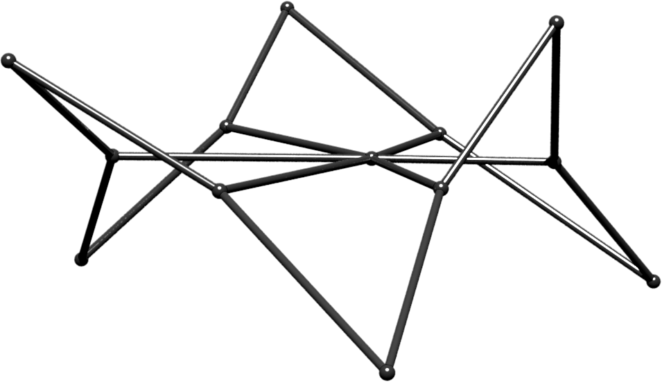
Figure 3. Edges adjacent to a vertex of a discrete A-net lie in a 2-plane.

Equivalence of vertex and contact element description of A-nets.

Recall, that contact elements in $\mathbb{R}\textup{P}^{3}$ can be written as $(\mathsf{x},\mathsf{P})$ (see Section 2.1). The two above descriptions are related as follows: Let $v$ and $w$ be two adjacent vertices of the quad graph $\mathcal{D}$, and $\mathsf{P}(v)$ and $\mathsf{P}(w)$ be the planes containing the respective vertices $\mathsf{f}(v)$ and $\mathsf{f}(w)$ of the A-net. Vertices and planes are encoded by the contact elements $L(v)=(\mathsf{f}(v),\mathsf{P}(v))$ and $L(w)=(\mathsf{f}(w),\mathsf{P}(w))$ in $\mathscr{L}^{3,3}$. The line $\mathsf{l}$ supporting the edge $(\mathsf{f}(v),\mathsf{f}(w))$ in $\mathbb{R}\textup{P}^{3}$ is exactly the intersection $l=L(v)\cap L(w)\in\mathcal{Q}^{3,3}$, cf. Fig. 4. We associate $l$ to the corresponding edge $(v,w)$ of $\mathcal{D}$. Those lines common to adjacent contact elements are called discrete asymptotic lines of the A-net. Representatives of the discrete asymptotic lines in $\mathbb{R}\textup{P}^{3,3}$ constitute the focal net of the discrete line congruence $L$. In the book of Bobenko and Suris [BS08] the definition of focal net is given for the regular $\mathbb{Z}^{2}$-grid. Hence there exist distinguished coordinate directions and they define multiple focal nets for different coordinate directions.

Figure 4. Discrete asymptotic lines of an A-net are the lines shared by adjacent contact elements.

Affine A-nets.

Note that, strictly speaking, in the projective setting there are no distinguished edges, i.e., line segments connecting adjacent vertices of an A-net. However, considering an A-net in an affine part $\mathbb{R}^{3}\subset\mathbb{R}\textup{P}^{3}$, there is a distinguished plane at infinity, and it is natural to connect the vertices of the A-net with finite edges as in Fig. 3. We call such A-nets equipped with finite edges affine A-nets.

Genericity assumption.

We assume that the A-nets under consideration are generic in the following sense. Discrete asymptotic lines are skew, except if they are adjacent to a common vertex. In terms of discrete congruences of isotropic lines in $\mathcal{Q}^{3,3}$, this means that two vertices of the focal net span an isotropic line if and only if they are associated with edges of $\mathcal{D}$ that are adjacent to a common vertex. Moreover, we assume that discrete asymptotic lines meeting at a vertex are distinct. This implies that the vertices of the focal net associated with an elementary quadrilateral of $\mathcal{D}$, i.e., representatives in $\mathbb{R}\textup{P}^{3,3}$ of the four discrete asymptotic lines of an elementary quadrilateral, span a 3-space in $\mathbb{R}\textup{P}^{3,3}$ (see Fig. 5).

Note that if one elementary quadrilateral of an A-net in $\mathbb{R}\textup{P}^{3}$ is contained in a 2-plane, the whole net has to be contained in this plane. In particular the A-net is not generic.

Notation for discrete maps.

A special instance of a quad-graph is (a piece of) $\mathbb{Z}^{2}$. In this case it is convenient to represent shifts in lattice directions by lower indices. For $z=(m,n)\in\mathbb{Z}^{2}$ and a map $\varphi$ on $\mathbb{Z}^{2}$ we write

$$\varphi_{1}(z):=\varphi(m+1,n),\ \varphi_{11}(z):=\varphi(m+2,n),\ \varphi_{2}(z):=\varphi(m,n+1),\quad\text{etc.}$$

However, also for a general quad-graph $\mathcal{D}$ we use indices as shift operators when talking about local properties, if the quad-graph can be identified locally with $\mathbb{Z}^{2}$.

Usually we omit the argument for discrete maps and write

$$\varphi=\varphi(z),\quad\varphi_{1}=\varphi_{1}(z)\quad\text{etc.}$$

The structure of A-nets as isotropic line congruences and the notation we use is shown in Fig. 5. Upper indices are used to denote the focal net. The lower index reflects the respective net direction.

Figure 5. Notation for a discrete congruence of lines $L$ and the corresponding focal net $h$, combinatorially and geometrically.

3.2. Pre-hyperbolic nets

Similar to the previous section, we give two descriptions of pre-hyperbolic nets, one in $\mathbb{R}\textup{P}^{3}$ and another one in $\mathbb{R}\textup{P}^{3,3}$ in terms of Pücker geometry. Then we show that an elementary quadrilateral of an A-net admits a 1-parameter family of adapted hyperboloids. Finally, we discuss the extension of A-nets to pre-hyperbolic nets and show in Theorem 14, that a simply connected A-net allows for such an extension, if and only if all interior vertices are of even degree. In this case there is a 1-parameter family of adapted pre-hyperbolic nets. As the name suggests, pre-hyperbolic nets are a first step towards hyperbolic nets. While hyperbolic nets contain hyperboloid surface patches associated with elementary quadrilaterals, for a pre-hyperbolic net the whole supporting hyperboloids are considered. The motivation to introduce pre-hyperbolic nets is two-fold. On the one hand, they provide a convenient way to prove the consistency of the extension of A-nets to hyperbolic nets. On the other hand they are interesting structures in their own right, especially in their Plücker geometric description. As we will see in Section 4, a hyperbolic net can be seen as a the restriction of a pre-hyperbolic net.

A generic discrete A-net with hyperboloids associated with elementary quadrilaterals is a pre-hyperbolic net, if

1. the four discrete asymptotic lines associated with edges of an elementary quadrilateral of the A-net are asymptotic lines of the corresponding hyperboloid, and

2. hyperboloids belonging to edge-adjacent quadrilaterals have coinciding contact elements along the common (discrete) asymptotic line $\mathsf{h}$, i.e., the hyperboloids are tangent along $\mathsf{h}$.

We translate i) and ii) to the projective model of Plücker geometry:

1. The four lines $\mathsf{h}^{(1)},\mathsf{h}^{(1)}_{2}$ and $\mathsf{h}^{(2)},\mathsf{h}^{(2)}_{1}$ associated with the edges of a quadrilateral of the A-net correspond to four points $h^{(1)},h^{(1)}_{2}$ and $h^{(2)},h^{(2)}_{1}$ on the Plücker quadric $\mathcal{Q}^{3,3}$, cf. Fig. 5. The hyperboloid $\mathcal{H}\subset\mathbb{R}\textup{P}^{3}$ associated with the quadrilateral corresponds to two polar planes $P^{(1)}$ and $P^{(2)}$ in $\mathbb{R}\textup{P}^{3,3}$ (cf. Theorem 3). Hence the edges of the quadrilateral are segments of asymptotic lines of the hyperboloid $\mathcal{H}$ if the points $h^{(1)},h^{(1)}_{2}$ resp. $h^{(2)},h^{(2)}_{1}$ lie in the plane $P^{(1)}$ resp. $P^{(2)}$.

2. Let $\mathcal{H}$ and $\mathcal{H}_{i}$ be the two hyperboloids associated with edge-adjacent quadrilaterals with associated planes $P^{(1)},P^{(2)}$ and $P^{(1)}_{i},P^{(2)}_{i}$, respectively. Then $\mathcal{H}$ and $\mathcal{H}_{i}$ are tangent at the common edge $h^{(j)}_{i},\ i\neq j$, (see Fig. 6) if all contact elements of the two hyperboloids along this edge coincide. So let $l^{(i)}\in P^{(i)}\cap\mathcal{Q}^{3,3}$ resp. $l^{(i)}_{i}\in P^{(i)}_{i}\cap\mathcal{Q}^{3,3}$ be two asymtotic lines of $\mathcal{H}$ resp. $\mathcal{H}_{i}$ through one point on the common edge. Then the contact elements $\operatorname{inc}[h^{(j)}_{i},l^{(i)}]$ and $\operatorname{inc}[h^{(j)}_{i},l^{(i)}_{i}]$ coincide, cf. Fig. 7. Hence $\mathcal{H}$ and $\mathcal{H}_{i}$ are tangent along the common edge if $\operatorname{inc}[h^{(j)}_{i},P^{(i)}]=\operatorname{inc}[h^{(j)}_{i},P^{(i)}_{i}]$

Figure 6. Lines and contact elements of edge-adjacent quadrilaterals of an A-net.

Figure 7. Planes $P^{(i)}$ and $P^{(i)}_{i}$ of adjacent hyperboloids $\mathcal{H}$ and $\mathcal{H}_{i}$ that are tangent along the common asymptotic line $h_{i}^{(j)}$ ($i\neq j$).

We use this insight for the definition of pre-hyperbolic nets in terms of Plücker geometry.

Definition 8 (Pre-hyperbolic net).

A generic discrete congruence of isotropic lines $L$ in $\mathcal{Q}^{3,3}$ defined on a quad-graph $\mathcal{D}$ with polar $2$-planes $P^{(1)},P^{(2)}\in\mathcal{P}_{\textrm{hyp}}$ associated with elementary quadrilaterals is a pre-hyperbolic net, if

1. $h^{(1)},h^{(1)}_{2}\in P^{(1)}$ and $h^{(2)},h^{(2)}_{1}\in P^{(2)}$, and

2. for hyperboloids associated with adjacent quadrilaterals $Q,Q_{i}$ of $\mathcal{D}$ as in Fig. 6, the subspaces $\operatorname{inc}[h^{(j)}_{i},P^{(i)}]$ and $\operatorname{inc}[h^{(j)}_{i},P_{i}^{(i)}]$ of $\mathbb{R}\textup{P}^{3,3}$ coincide for $i\neq j$, cf. Fig. 7.

Remark 9.

Property ii) in Definition 8 implies that corresponding reguli of adjacent hyperboloids have the same orientation. In Fig. 7, if the signature of $P^{(i)}$ is $({+}{+}{-})$, then the 3-space $\operatorname{inc}[h_{i}^{(j)},P^{(i)}]$ is of (degenerate) signature $({+}{+}{-}{0})$. Since $P_{i}^{(i)}$ does not contain $h_{i}^{(j)}$, the plane $P_{i}^{(i)}$ is also of signature $({+}{+}{-})$. The fact that the two reguli of a single hyperboloid are of complementary signature in turn implies, that $P^{(j)}$ and $P_{i}^{(j)}$ also have the same signature.

Extending discrete A-nets to pre-hyperbolic nets.

For an elementary quadrilateral $Q=(L,L_{1},L_{12},L_{2})$ of an A-net we define

$$\operatorname{inc}[Q] := \operatorname{inc}[L,L_{1},L_{12},L_{2}],$$

$$H[Q] := \operatorname{pol}[L,L_{1},L_{12},L_{2}]=\operatorname{pol}[Q].$$

Usually we write $H,H_{i}$ for $H[Q],H[Q_{i}]$, etc.

Proposition 10.

Let $Q$ be an elementary quadrilateral of a generic A-net that is defined on a quad-graph $\mathcal{D}$. Then:

1. The space $\operatorname{inc}[Q]\subset\mathbb{R}\textup{P}^{3,3}$ is 3-dimensional and of signature $({+}{+}{-}{-})$. The space $H[Q]\subset\mathbb{R}\textup{P}^{3,3}$ is a projective line of signature $(+-)$.

2. The lines $H=\operatorname{pol}[Q]$ associated with the elementary quadrilaterals $Q$ of the A-net constitute a discrete line congruence on the dual graph of $\mathcal{D}$.

Proof.

i) An elementary quadrilateral of a generic A-net is a non-planar quadrilateral in $\mathbb{R}\textup{P}^{3}$. According to Remark 2, the pairs $h^{(2)},h^{(2)}_{1}$ and $h^{(1)},h^{(1)}_{2}$, as well as the diagonals $g_{1},g_{2}$ each span lines of signature $(+-)$ in $\mathbb{R}\textup{P}^{3,3}$. So $H[Q]=\operatorname{inc}[g_{1},g_{2}]$ has signature $(+-)$ and thus its polar $\operatorname{inc}[Q]$ has signature $({+}{+}{-}{-})$.

ii) It remains to show that for edge-adjacent quadrilaterals $Q$ and $Q_{i}$ the lines $H$ and $H_{i}$ intersect. This follows from the observation, that $L_{i}$ and $L_{ij}$, $i\neq j$, are both contained in each of the projective spaces $\operatorname{inc}[Q]$ and $\operatorname{inc}[Q_{i}]$, and hence $H,H_{i}\subset\operatorname{pol}[L_{i},L_{ij}]$, cf. Fig. 6. Since $\operatorname{pol}[L_{i},L_{ij}]$ is a projective plane, the lines $H$ and $H_{i}$ intersect. ∎

Each of the elementary quadrilaterals admits a 1-parameter family of adapted hyperboloids as indicated in Fig. 9. These hyperboloid can be described in terms of Plücker geometry as explained in the following Lemma 11.

Lemma 11.

For an elementary quadrilateral $Q$ of a generic A-net there is a 1-parameter family of hyperboloids containing all four discrete asymptotic lines. Each such hyperboloid is uniquely determined by the choice of two labeled points $q^{(1)},q^{(2)}\in H[Q]$ that are polar (see Fig. 9 left).

Proof.

For each non-isotropic point $q\in H=H[Q]$ there is a unique polar point on $H$, due to the signature $(+-)$ of $H$. Each pair of polar points $q^{(1)},q^{(2)}\in H\setminus\mathcal{Q}^{3,3}$ determines a pair of polar planes $P^{(i)}:=\operatorname{inc}[h^{(i)},h^{(i)}_{j},q^{(i)}]$ in $\mathcal{P}_{\textrm{hyp}}$. These planes define a unique hyperboloid with prescribed asymptotic lines, cf. Fig. 8. Conversely, any hyperboloid $\mathcal{H}$ that contains the given discrete asymptotic lines can be constructed in this way, since associated polar planes $P^{(i)}\in\mathcal{P}_{\textrm{hyp}}$ intersect $H$ in polar points $q^{(i)}$. ∎

Figure 8. Configuration in $\mathbb{R}\textup{P}^{3,3}$ which describes the extension of an elementary quadrilateral of a discrete A-net to a hyperboloid. Given representatives $h^{(1)},h_{2}^{(1)},h^{(2)},h_{1}^{(2)}\in\mathcal{Q}^{3,3}$ of the discrete asymptotic lines, the extension is performed by choosing polar points $q^{(1)},q^{(2)}\in H$.

Remark 12.

There are two special choices for $q\in H$, namely the isotropic points in $H\cap\mathcal{Q}^{3,3}$. In this case, $\mathsf{q}$ is one of the two diagonals of the non-planar quadrilateral in $\mathbb{R}\textup{P}^{3}$. Furthermore, $q$ is self polar and does not yield a decomposition of $\mathbb{R}\textup{P}^{3,3}$ into two disjoint planes in $\mathcal{P}_{\textrm{hyp}}$ as required by Theorem 3. Hence there is no hyperboloid associated with $q=q^{(1)}=q^{(2)}$. Instead this choice corresponds to one of the two limiting cases of hyperboloids $\mathcal{H}$ for which $\mathsf{h}^{(1)},\mathsf{h}_{2}^{(1)},\mathsf{h}^{(2)},\mathsf{h}_{1}^{(2)}$ are asymptotic lines. The hyperboloid degenerates to two planes in $\mathbb{R}\textup{P}^{3}$ that contain those lines and intersect in the diagonal $\mathsf{q}$ (see Fig. 9 right). Considering $P^{(1)}=\operatorname{inc}[h^{(1)},h_{2}^{(1)},q]$ and $P^{(2)}=\operatorname{inc}[h^{(2)},h_{1}^{(2)},q]$ as for hyperboloids, each intersection $P^{(i)}\cap\mathcal{Q}^{3,3}$ with the Plücker quadric gives a degenerate conic. These degenerate conics each consist of two isotropic lines, i.e., two contact elements. The planes of these contact elements are exactly the planes in $\mathbb{R}\textup{P}^{3}$ intersecting in $\mathsf{q}$, and the points of the contact elements are the vertices of the quadrilateral that are adjacent to $\mathsf{q}$.

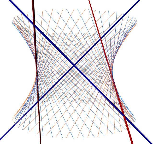
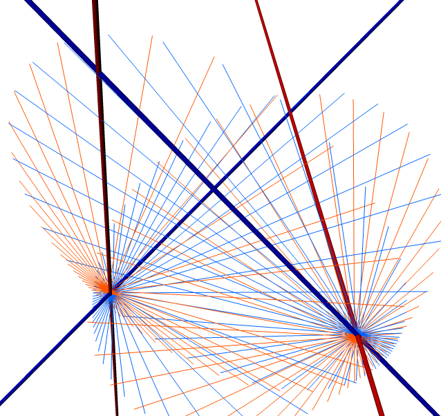
Figure 9. The 1-parameter family of adapted hyperboloids supporting an elementary quadrilateral of an A-net: Two non-degenerate hyperboloids (left) and the two degenerate cases (right).

The $C^{1}$-condition for adjacent hyperboloids in a pre-hyperbolic net determines the whole net if one initial hyperboloid is given. In particular, there exists a 1-parameter family of pre-hyperbolic nets for a generic discrete A-net. To prove consistency of the evolution, we first describe the propagation of a hyperboloid from one quadrilateral to an adjacent one as a projection between $H$ and $H_{i}$.

Lemma 13.

For a pre-hyperbolic net let $Q$ and $Q_{i}$ be edge-adjacent quadrilaterals of the underlying A-net. Then the line $H_{i}=H[Q_{i}]$ is the projection of $H=H[Q]$ onto $\operatorname{pol}[h_{ii}^{(j)}]$ through the point $h_{i}^{(j)},i\neq j$. In particular, the points $q^{(1)}$ and $q^{(2)}$ are mapped onto $q_{i}^{(1)}$ and $q_{i}^{(2)}$, cf. Fig. 10.

Figure 10. For pre-hyperbolic nets, $H_{i}$ is the projection of $H$ onto $\operatorname{pol}[h_{ii}^{(j)}]$ through $h_{i}^{(j)}$. In particular $(q^{(1)},q^{(2)})$ is mapped to $(q_{i}^{(1)},q_{i}^{(2)})$ and $h_{i}^{(j)}$ lies in the plane $\operatorname{inc}[H,H_{i}]$.

Proof.

For generic A-nets, the point $h_{i}^{(j)}\in\mathcal{Q}^{3,3}$, $i\neq j$, is not contained in $\operatorname{pol}[h_{ii}^{(j)}]$ and the projection

(1) $$\tau:\mathbb{R}\textup{P}^{3,3}\setminus\{h_{i}^{(j)}\} \to \operatorname{pol}[h_{ii}^{(j)}]$$

$$q \mapsto \operatorname{inc}[q,h_{i}^{(j)}]\cap\operatorname{pol}[h_{ii}^{(j)}]$$

through $h_{i}^{(j)}$ is well defined. It is crucial that $\tau$ maps $\operatorname{pol}[h_{i}^{(j)}]$ onto $\operatorname{pol}[h_{i}^{(j)}]\cap\operatorname{pol}[h_{ii}^{(j)}]$. The reason is that $h_{i}^{(j)}$ is isotropic, and hence for all $q\in\operatorname{pol}[h_{i}^{(j)}]$ the projection line $\operatorname{inc}[q,h_{i}^{(j)}]$ is completely contained in $\operatorname{pol}[h_{i}^{(j)}]$. Since for a pre-hyperbolic net $\operatorname{inc}[P^{(i)},h_{i}^{(j)}]=\operatorname{inc}[P_{i}^{(i)},h_{i}^{(j)}]$, the space $P^{(i)}\subset\operatorname{pol}[h_{i}^{(j)}]$ is mapped to $P_{i}^{(i)}\subset\operatorname{pol}[h_{i}^{(j)}]\cap\operatorname{pol}[h_{ii}^{(j)}]$, cf. Fig. 7. This means

(2) $$\tau(P^{(i)})=P_{i}^{(i)}$$

and in particular

(3) $$\tau(h^{(i)})=h_{i}^{(i)}\quad\text{and}\quad\tau(h_{j}^{(i)})=h_{ij}^{(i)}.$$

The claim of the Lemma

(4) $$\tau(H)=H_{i}$$

holds, since $\tau$ preserves polarity: Let $q,q^{\prime}\in\operatorname{pol}[h_{i}^{(j)}]$ with $\langle\widehat{q},\widehat{q}^{\prime}\rangle=0$. Thus for all $\alpha,\alpha^{\prime},\beta,\beta^{\prime}\in\mathbb{R}$ we have

$$\langle\alpha\,\widehat{q}+\beta\,\widehat{h}_{i}^{(j)},\alpha^{\prime}\,\widehat{q}^{\prime}+\beta^{\prime}\,\widehat{h}_{i}^{(j)}\rangle=0\quad\Rightarrow\quad\tau(q),\tau(q^{\prime})\text{ are polar}.$$

With Eq. (3) and definition of $\tau$ this implies that $\operatorname{pol}[h_{i}^{(j)},h^{(i)},h_{j}^{(i)}]\supset H$ is mapped onto $\operatorname{pol}[h_{i}^{(j)},h_{i}^{(i)},h_{ij}^{(i)},h_{ii}^{(j)}]=H_{i}$. Together with Eq. (2) and Eq. (3), preservation of polarity also implies that $q^{(i)}$ (the unique point in $P^{(i)}$ that is polar to $h^{(i)}$ and $h_{j}^{(i)}$, cf. Fig. 8) is mapped to $q_{i}^{(i)}$ (the unique point in $P_{i}^{(i)}$ that is polar to $h_{i}^{(i)}$ and $h_{ij}^{(i)}$). Finally the preservation of polarity toghether with Eq. (4) gives $\tau(q^{(j)})=q_{i}^{(j)}$. ∎

We are now ready to proof the main theorem about pre-hyperbolic nets.

Theorem 14.

For a given simply connected generic A-net with all interior vertices of even degree, there exists a 1-parameter family of pre-hyperbolic nets. Each such net is determined by the choice of one initial hyperboloid.

Proof.

Lemma 11 shows that for each elementary quadrilateral of an A-net, there is a 1-parameter family of compatible hyperboloids. Hence we have a 1-parameter freedom for the choice of one initial hyperboloid. Lemma 13 explains how this hyperboloid determines its four neighboring hyperboloids associated with edge-adjacent quadrilaterals. It remains to show that this evolution is consistent, i.e., that the propagation of hyperboloids is independent of the particular chosen path. Since the quad-graph is simply connected, there are no non-trivial cycles. Thus we have to consider consistency of the evolution around single inner vertices only.

Figure 11. All four projection centers $h_{i}^{(j)}$ lie on the line $L_{12}$.

First, we consider a regular vertex of degree four as in Fig. 11. We start with the two points $q^{(1)}$ and $q^{(2)}$ on $H=\operatorname{pol}[Q]$, which determine the hyperboloid $\mathcal{H}$ associated with the lower left quadrilateral. By Lemma 13, the projections of $(q^{(1)},q^{(2)})$ onto $H_{1}$ and $H_{2}$ according to Eq. (1) yield the adjacent hyperboloids $\mathcal{H}_{1}$ and $\mathcal{H}_{2}$, respectively. Consistency for all initial data means that the map used for propagation of the pair $(q^{(1)},q^{(2)})$ around the vertex is the identity. More precisely, we have to check whether the evolution satisfies two properties. Firstly, according to the notation of Lemma 13, it has to hold

(5) $$\tau_{2}^{(1)}\circ\tau_{12}^{(2)}\circ\tau_{12}^{(1)}\circ\tau_{1}^{(2)}=\mathrm{id}\quad\Leftrightarrow\quad\tau_{12}^{(1)}\circ\tau_{1}^{(2)}=\tau_{12}^{(2)}\circ\tau_{2}^{(1)},$$

where lower and upper indices correspond to the center of projection. Here $\tau_{2}^{(1)},\tau_{12}^{(2)},\tau_{12}^{(1)},\tau_{1}^{(2)}$ are understood as involutions, for example the projection $\tau_{1}^{(2)}:H\to H_{1}$ through $h_{1}^{(2)}$ as map in $\mathbb{R}\textup{P}^{3,3}$ is inverted by exchanging domain and co-domain (cf. Fig. 10). Moreover, we have to prove that the labeling of $q$’s is preserved.

To prove Eq. (5), first note that by definition of the lines $H,H_{1},H_{12},H_{2}$, the space $V=\operatorname{inc}[H,H_{1},H_{12},H_{2}]$ is contained in the 3-space $\operatorname{pol}[L_{12}]\supset L_{12}$. Moreover, $\operatorname{inc}[H,H_{1}]\cap L_{12}=h_{1}^{(2)}$ and similarly for the other $H$-lines, cf. Fig. 10. As the four intersection points $h_{1}^{(2)},h_{12}^{(1)},h_{12}^{(2)},h_{2}^{(1)}\in L_{12}$ are distinct, the space $V$ has to be at least 3-dimensional and hence $V=\operatorname{pol}[L_{12}]$. As a consequence we can restrict ourselves to the projective 3-space $V$ and understand the projections $\tau_{2}^{(1)},\tau_{12}^{(2)},\tau_{12}^{(1)},\tau_{1}^{(2)}$ as one and the same projection $\tau$ through $L_{12}$, just acting on different (co-)domains. This proves Eq. (5).

So far, exactly the same argumentation holds for arbitrary degree of the central vertex greater than 4 and the corresponding identities analogous to (5). However, in contrast to that, the labeling of $q$’s is only preserved for even vertex degree: Given a point $q\in H=\operatorname{pol}[Q]$ one can understand the labeling $q\to q^{(i)}$ as association of $q$ to an edge that is adjacent to the central vertex, say $v$, since the two edges of $Q$ adjacent to $v$ are natural representatives of the two reguli of any admissible hyperboloid. Now if $q$ is propagated $q\mapsto q_{i}=\tau_{i}^{(j)}(q)$, then the labeling, i.e., allocation of $q$ to an edge adjacent to $v$, has to be propagated accordingly (cf. Fig. 12). It follows, that the labeling of $q$’s is propagated consistently, if and only if $v$ is of even degree. ∎

Figure 12. Propagation of the labeling of $q$’s with respect to the map $\tau_{1}^{(2)}$, represented by edges adjacent to the central vertex.

Remark 15.

A simply connected quad-graph is either a disc or a sphere, in particular it is orientable. Moreover, if all interior vertices are of even degree, it has to be a disc. This follows from the Euler characteristic, which yields that a strongly regular cell-decomposition of a sphere necessarily contains either triangles or vertices of degree $3$. One can also show this way, that the considered quad-graphs do not contain self-intersecting or closed quadrilateral strips (see Definition 20).

4. Hyperbolic nets

This section aims at the extension of affine A-nets to piecewise smooth $C^{1}$-surfaces, called hyperbolic nets. An A-net in $\mathbb{R}\textup{P}^{3}$ is turned into an affine A-net by choosing an affine chart of $\mathbb{R}\textup{P}^{3}$ and equipping the A-net with finite edges connecting adjacent vertices, see Section 3.1. The elementary quadrilaterals of affine A-nets are therefore skew quadrilaterals in $\mathbb{R}^{3}$. Extending an affine A-net to a hyperbolic net amounts to fitting hyperboloid surface patches into the skew quadrilaterals in such a way that the connection between edge-adjacent patches are differentiable. Related to the propagation of hyperboloids in pre-hyperbolic nets, a surface patch glued to a skew quadrilateral determines its edge-adjacent neighbors via the $C^{1}$-property. Starting with one initial hyperboloid patch, the consistency of this propagation is derived from the consistency of the propagation of hyperboloids for pre-hyperbolic nets. It turns out that not all affine A-nets that allow for an extension to pre-hyperbolic nets can also be extended to hyperbolic nets. The additional characteristic property is shown to be “equi-twist” of quadrilateral strips.

We discuss the orientation of reguli and introduce the related twist of skew quadrilaterals in Section 4.1. In Section 4.2, we first investigate hyperboloid surface patches focussing on patches bounded by a prescribed skew quadrilateral. Then we introduce hyperbolic nets and show how to construct hyperbolic nets from affine A-nets in Theorem 21. Finally, some comments are made on the computer implementation of our results.

4.1. Orientation of reguli and twist of skew quadrilaterals

Any three skew lines in $\mathbb{R}\textup{P}^{3}$ span a regulus. The corresponding plane in $\mathcal{P}_{\textrm{hyp}}$ is either of signature $({+}{+}{-})$ or of signature $({+}{-}{-})$, where the different signatures correspond to the two possible orientations of reguli. Hence an orientation in $\mathbb{R}\textup{P}^{3}$ is defined for three skew lines. A skew quadrilateral in $\mathbb{R}\textup{P}^{3}$ consists of four points in general position connected by line segments (edges). The notion of orientation for reguli induces a natural orientation for a pair of opposite edges of a skew quadrilateral. We call this orientation the twist of an opposite edge pair.

Orientation of reguli.

Consider a hyperboloid $\mathcal{H}$ in $\mathbb{R}\textup{P}^{3}$ that is described by two polar planes $P^{(1)}$ and $P^{(2)}$ in $\mathbb{R}\textup{P}^{3,3}$, which are spanned by representatives of arbitrary three lines of the corresponding reguli of $\mathcal{H}$. Assume $P^{(1)}$ is of signature $({+}{+}{-})$ and $P^{(2)}$ is of signature $({+}{-}{-})$. The signature of a plane $P$ is the signature of the Plücker product restricted to the 3-space $\widehat{P}$ of homogeneous coordinates. With respect to a particular basis, the restriction $\langle\cdot,\cdot\rangle\big{|}_{\widehat{P}}$ is represented by a symmetric $3\times 3$ matrix $M_{P}$, cf. Appendix A. Due to Sylvester’s law of inertia, the signature of $M_{P}$ is independent of the chosen basis and coincides with the signature of $\langle\cdot,\cdot\rangle\big{|}_{\widehat{P}}$. As the determinant of a matrix is the product of its eigenvalues, we have

$$\det(M_{P^{(1)}})<0\quad\text{and}\quad\det(M_{P^{(2)}})>0.$$

According to the sign of the determinant, the regulus $P^{(1)}\cap\mathcal{Q}^{3,3}$ is said to be of negative orientation, while $P^{(2)}\cap\mathcal{Q}^{3,3}$ is said to be of positive orientation. For the calculation of the orientation of a regulus (or, equivalently, the orientation of three skew lines) in coordinates, see Appendix A.

Remark 16.

There are different choices of Plücker line coordinates, and the orientation of a regulus (of three skew lines) depends on the particular choice. In a fixed affine chart, one can identify the two possible orientations of reguli with clockwise and counter-clockwise screw motions in space. However, this interpretation depends on the choice of the affine chart – while for fixed Plücker coordinates the orientation of a regulus is well defined, in different affine charts the same regulus may appear rotating either clockwise or counter-clockwise.

Now recall the extension of an elementary quadrilateral $Q$ of an A-net to a hyperboloid, as discussed in Section 3.2. By Lemma 11 there exists a 1-parameter family of different hyperboloids, whose asymptotic lines contain the discrete asymptotic lines of the A-net (see Fig. 9). The 1-parameter family of hyperboloids corresponds to the 1-parameter family of polar points $q,q^{*}\in H[Q]=\operatorname{pol}[h^{(1)},h^{(1)}_{2},h^{(2)},h^{(2)}_{1}]$. We ignore the degenerate case $q=q^{*}$, which is equivalent to $\langle\widehat{q},\widehat{q}\rangle=0$ (see Remark 12). In the generic case $\langle\widehat{q},\widehat{q}\rangle$ and $\langle\widehat{q}^{*},\widehat{q}^{*}\rangle$ have opposite signs. Such a generic pair of polar points yields two different hyperboloids, depending on the labeling of the points, i.e., either $q^{(1)}=q$ and $q^{(2)}=q^{*}$ or the other way around. The essential difference between the labelings is the following: Changing the labeling also changes the signatures of $P^{(1)}=\operatorname{inc}[h^{(1)},h^{(1)}_{2},q^{(1)}]$ and $P^{(2)}=\operatorname{inc}[h^{(2)},h^{(2)}_{1},q^{(2)}]$, i.e., the orientation of the hyperbolic families of lines $P^{(1)}\cap\mathcal{Q}^{3,3}$ and $P^{(2)}\cap\mathcal{Q}^{3,3}$.

As mentioned in Remark 16, in a fixed affine chart the orientation of a regulus can be described as a clockwise or counter-clockwise screw motion. We will now explain this geometric interpretation in the context of the extension of a quadrilateral of an A-net to an adapted hyperboloid. Extending the pair of lines $\mathsf{h}^{(1)}$ and $\mathsf{h}_{2}^{(1)}$ to a regulus of an adapted hyperboloid corresponds to choosing a third line $\mathsf{h}$ that is skew to $\mathsf{h}^{(1)}$ and $\mathsf{h}_{2}^{(1)}$, but that intersects $\mathsf{h}^{(2)}$ and $\mathsf{h}_{1}^{(2)}$, cf. Fig. 13. Referring to the affine chart used in Fig. 13, the regulus $\mathcal{H}^{(1)}=\operatorname{inc}[h^{(1)},h,h_{2}^{(1)}]\cap\mathcal{Q}^{3,3}$ is oriented clockwise. This reflects how the lines of $\mathcal{H}^{(1)}$ twist around any line of the complementary regulus $\mathcal{H}^{(2)}=\operatorname{pol}[h^{(1)},h,h_{2}^{(1)}]\cap\mathcal{Q}^{3,3}$. In particular, the twist direction is independent of whether you choose $\mathsf{h}^{(2)}$, or $\mathsf{h}_{1}^{(2)}$ as reference. It is also independent of the direction of traversal of the reference line. (Keep in mind that every two lines of one regulus of a hyperboloid are skew. Hence for each regulus there is a unique screw motion that identifies three lines of a regulus.) If one considers the regulus $\tilde{\mathcal{H}}^{(1)}=\operatorname{inc}[h^{(1)},\tilde{h},h_{2}^{(1)}]\cap\mathcal{Q}^{3,3}$, that is spanned by the skew lines $\mathsf{h}^{(1)},\mathsf{\tilde{h}}$, and $\mathsf{h}_{2}^{(1)}$ instead, then $\tilde{\mathcal{H}}^{(1)}$ is oriented counter-clockwise.

Figure 13. With respect to a fixed affine chart, the orientation of a regulus can be referred to as a clockwise or counter-clockwise screw motion. The regulus spanned by $\mathsf{h}^{(1)},\mathsf{h},\mathsf{h}_{2}^{(1)}$ is oriented clockwise, while the regulus spanned by $\mathsf{h}^{(1)},\mathsf{\tilde{h}},\mathsf{h}_{2}^{(1)}$ is oriented counter-clockwise.

Twist of skew quadrilaterals.

Any skew quadrilateral in $\mathbb{R}\textup{P}^{3}$ can be seen as a skew quadrilateral in $\mathbb{R}^{3}$, i.e., there is an affine chart such that all four edges of the quadrilateral are finite. Accordingly, consider Fig. 13 in affine $\mathbb{R}^{3}$, such that there is a unique skew quadrilateral with vertices $\mathsf{x}$, $\mathsf{x}_{1}$, $\mathsf{x}_{2}$, and $\mathsf{x}_{12}$ and finite edges connecting them. The twist of the opposite edge pair $(\mathsf{x},\mathsf{x}_{1})$ and $(\mathsf{x}_{2},\mathsf{x}_{12})$ is defined as the orientation of any regulus that is spanned by $\mathsf{h}^{(1)},\mathsf{h}^{(1)}_{2}$, and a third line $\mathsf{h}$, where $\mathsf{h}$ is skew to $\mathsf{h}^{(1)},\mathsf{h}^{(1)}_{2}$ but intersects the complementary lines $\mathsf{h}^{(2)}$ and $\mathsf{h}^{(2)}_{1}$ in their finite segments, i.e., in the edges of $Q$. So the twist of an opposite edge pair can be either positive, or negative. Intuitively it is clear, that the twist does not depend on the particular choice of the line $\mathsf{h}$; a proof using coordinates can be found in Appendix A. The other edge pair, $(\mathsf{x},\mathsf{x}_{2})$ and $(\mathsf{x}_{1},\mathsf{x}_{12})$, automatically has the opposite twist.

4.2. Hyperbolic nets

In Section 3 it was shown that simply connected A-nets with all interior vertices of even degree can be extended to pre-hyperbolic nets. Now we will characterize affine A-nets that can be extended to piecewise smooth $C^{1}$-surfaces parametrized along asymptotic lines, by attaching hyperboloid patches to the skew quadrilaterals. The resulting surfaces are called hyperbolic nets. We start with the formal definition of hyperboloid patches and the extension of skew quadrilaterals to such patches, before defining hyperbolic nets similar to pre-hyperbolic nets.

Definition 17 (Hyperboloid patch).

A hyperboloid patch is a (parametrized) surface patch, obtained by restricting a (global) asymptotic line parametrization of a hyperboloid to a closed rectangle.

Geometrically, a hyperboloid patch is a piece of a hyperboloid cut out along four asymptotic lines, two per regulus, cf. Fig. 14. Conversely, four asymptotic lines of a hyperboloid cut the hyperboloid into four patches, since a hyperboloid in $\mathbb{R}\textup{P}^{3}$ is a torus, topologically. If we choose a plane at infinity, then this plane intersects some, or all of the patches. More precisely, in the affine setting a hyperboloid is cut by four asymptotic lines into either four infinite patches or into three infinite patches and one finite patch.

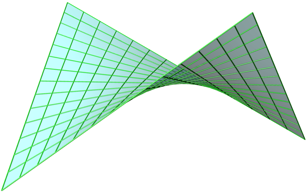
Figure 14. Left: A finite hyperboloid patch. Right: A finite skew quadrilateral on a hyperboloid that does not bound a hyperboloid patch.

Using the results of Section 4.1, we will now discuss the extension of skew quadrilaterals to hyperboloid patches. Lemma 11 tells us, that for a skew quadrilateral $Q$ there exists a 1-parameter family of adapted hyperboloids. The crucial observation is, that such a hyperboloid can be restricted to a hyperboloid patch that is bounded by $Q$, if and only if the twists of the opposite edge pairs of $Q$ coincide with the corresponding orientations of the reguli of $\mathcal{H}$, cf. Fig. 14. The reason for that is, that there is a patch bounded by $Q$, if and only if asymptotic lines of $\mathcal{H}$ that intersect one edge of $Q$ also intersect the opposite edge of $Q$ (recall the definition of the twist of opposite edge pairs and consider Fig. 13). If the twist of one opposite edge pair coincides with the orientation of the supporting regulus, this is obviously also the case for the other edge pair. If the edges of $Q$ are finite, then any patch bounded by $Q$ is also finite, cf. Fig. 15.

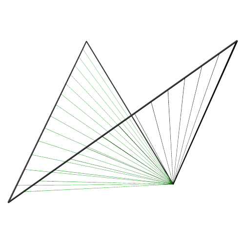
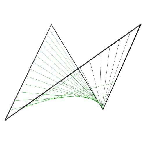
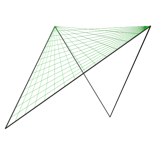
Figure 15. Hyperboloid patches adapted to a skew quadrilateral.

We summarize the above in the following Lemma 18

Lemma 18.

Let $\mathcal{H}$ be a hyperboloid and $Q$ be a skew quadrilateral on $\mathcal{H}$. The hyperboloid can be restricted to a hyperboloid patch that is bounded by $Q$, if and only if the twist of each opposite edge pair of $Q$ coincides with the orientation of the regulus of $\mathcal{H}$ containing the edge pair. If twist and orientation coincide for one pair, they coincide for the other pair as well. The restriction is unique, if it exists. With respect to an affine chart the obtained patch is finite, if and only if $Q$ is finite.

Finally, we arrive at the definition of our main object of interest – affine A-nets extended to piecewise smooth $C^{1}$-surfaces by gluing hyperboloid patches into the skew quadrilaterals.

Definition 19 (Hyperbolic net).

A generic discrete affine A-net with hyperboloid patches associated with the elementary quadrilaterals is a hyperbolic net, if

1. the edges of the quadrilaterals are the bounding asymptotic lines of the hyperboloid patches,

2. the surface composed of the hyperboloid patches is a piecewise smooth $C^{1}$-surface.

As mentioned before, there exist affine A-nets that cannot be extended to hyperbolic nets, even though there exists a 1-parameter family of pre-hyperbolic nets. The characterizing property for affine A-nets to be extendable to hyperbolic nets is given in the following definition.

Definition 20 (Quad-strip / equi-twisted strips).

A sequence $\{Q_{i}\}_{i=1,\dots,n}$ of quadrilaterals in a quadrilateral mesh, such that the edges $l_{i}=Q_{i-1}\cap Q_{i}$ and $r_{i}=Q_{i}\cap Q_{i+1}$ are opposite edges in $Q_{i}$, is called strip (cf. Fig. 16). A strip of an A-net is equi-twisted if the edge pairs $(l_{i},r_{i})$ have the same twist for all skew quadrilaterals along the strip (see Section 4.1).

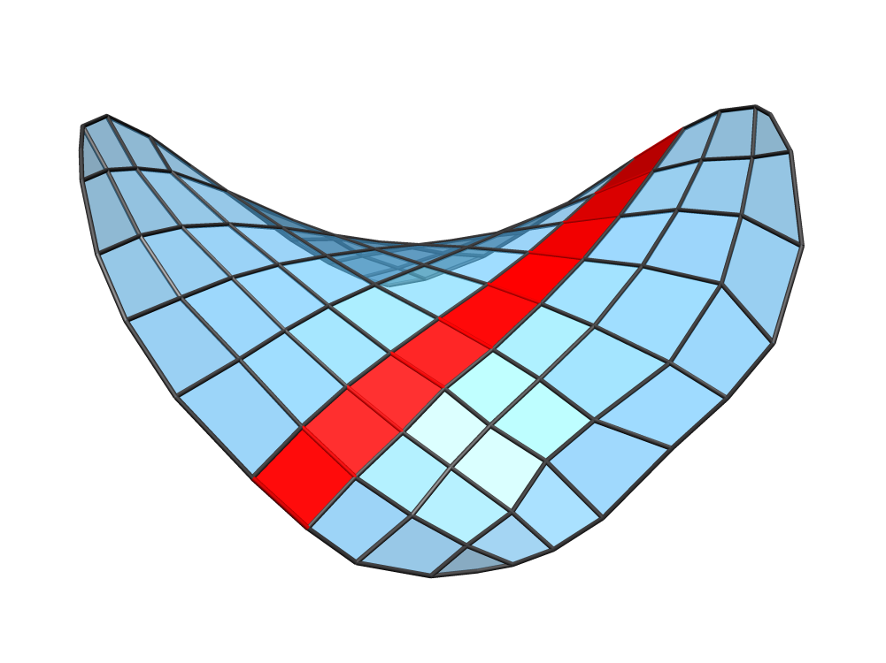
Figure 16. An equi-twisted strip of an A-net.

Definition 20 is motivated by the propagation of the hyperboloids for pre-hyperbolic nets, since the signatures of corresponding reguli are preserved by the propagation (see Remark 9). We obtain the following characterization of those affine A-nets that can be extended to hyperbolic nets.

Theorem 21.

A simply connected generic affine A-net can be extended to a hyperbolic net, if and only if the strips of the A-net are equi-twisted. In this case there exists a 1-parameter family of adapted hyperbolic nets. Each such net is determined by the choice of one initial hyperboloid patch that is bounded by one arbitrary skew quadrilateral of the A-net.

Proof.

First observe, that in an A-net with equi-twisted strips all interior vertices necessarily have even vertex degree, because the two pairs of opposite edges of a skew quadrilateral have opposite twists. The rest follows from Theorem 14 together with Lemma 18 and Remark 9. ∎

Computer implementation.

The generation of hyperbolic nets has been implemented in java, using jReality [jG]. Starting with an arbitrary quadrilateral mesh of suitable combinatorics as input, the first step is to turn the mesh into an A-net. This is achieved by a variational approach, in which the non-planarity of vertex stars is minimized. The corresponding functional $\mathcal{S}$ is a sum of volumes of tetrahedra. The sum covers all possible tetrahedra $\Delta$ that are spanned by vertices of the mesh, under the restriction that for each tetrahedron the four vertices have to be contained in a single vertex star

$$\mathcal{S}=\sum_{v\in V}\sum_{v_{1},\ldots,v_{4}\in\operatorname{star}(v)}\operatorname{Vol}(\Delta(v_{1},v_{2},v_{3},v_{4})).$$

To extend the obtained A-net to a hyperbolic net, we have to choose an initial hyperboloid patch for some quadrilateral. As described in the previous section we define the initial patch by choosing a point $q\in\mathbb{R}\textup{P}^{3,3}$ on the line spanned by the representatives of the two diagonals of the initial skew quadrilateral. The initial patch is then propagated automatically to all other quadrilaterals and one obtains a piecewise smooth $C^{1}$-surface, parametrized as shown in Fig. 17.

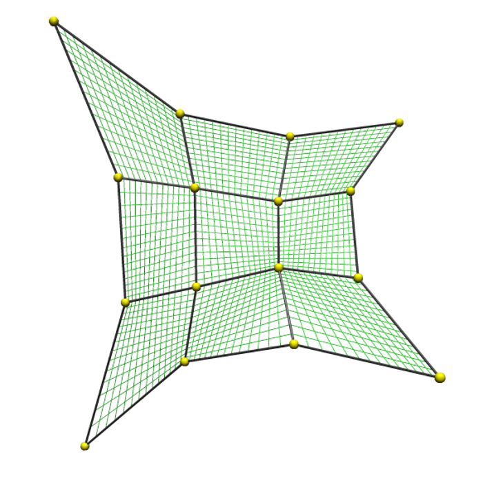
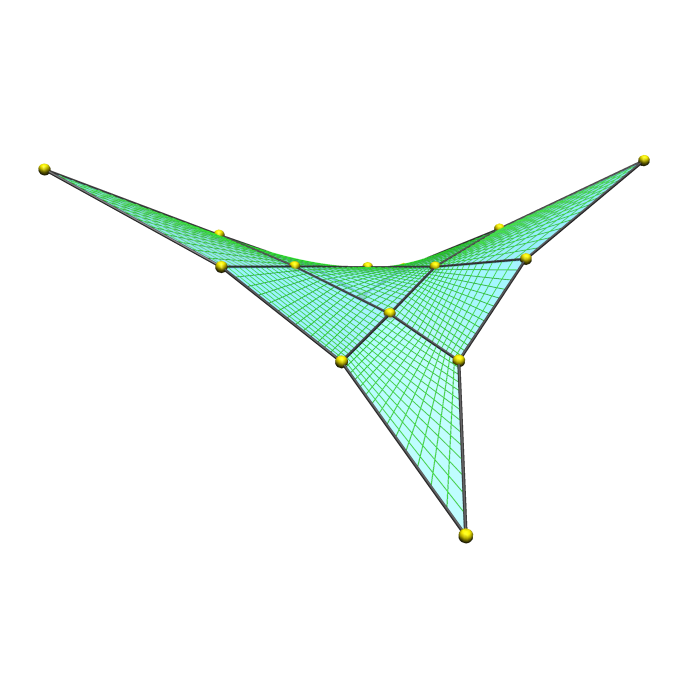
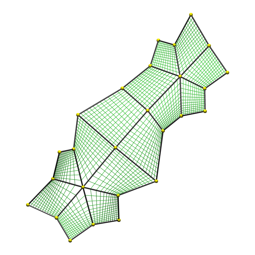
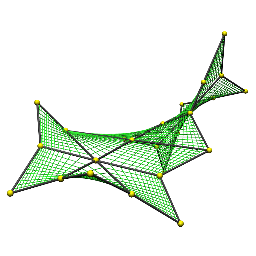
Figure 17. Examples of hyperbolic nets. The top one is of regular $\mathbb{Z}^{2}$ combinatorics, while the bottom one has two degree six vertices.

Appendix A

In contrast to the main text, we will now use the exterior algebra model of Plücker geometry (see, for example, [PW01] or [BS08]) to do explicit calculations with points and lines.

Using exterior algebra, Plücker line coordinates arise in a very natural way if a basis of the space $\mathbb{R}^{4}$ of homogeneous coordinates for $\mathbb{R}\textup{P}^{3}$ has been chosen. The space of line coordinates in the exterior algebra description is $\Lambda^{2}(\mathbb{R}^{4})$, so the projective space containing the Plücker quadric becomes $\operatorname{P}(\Lambda^{2}(\mathbb{R}^{4}))$. The wedge product on $\mathbb{R}^{4}$ gives Plücker coordinates of lines, i.e., the line $\mathsf{h}$ spanned by two points $\mathsf{x},\mathsf{y}\in\mathbb{R}\textup{P}^{3}$ has Plücker coordinates

$$h=\widehat{\mathsf{x}}\wedge\widehat{\mathsf{y}}\in\Lambda^{2}(\mathbb{R}^{4}).$$

Scaling homogenous coordinates $\widehat{\mathsf{x}},\widehat{\mathsf{y}}$ by non-zero factors obviously just results in a corresponding scaling of $h$.

The wedge product on $\Lambda^{2}(\mathbb{R}^{4})$ is exactly the Plücker product (after canonical identification of $\Lambda^{4}(\mathbb{R}^{4})$ with $\mathbb{R}$). Two lines $\mathsf{h}=\operatorname{inc}[\mathsf{x},\mathsf{y}]$ and $\mathsf{l}=\operatorname{inc}[\mathsf{u},\mathsf{v}]$ in $\mathbb{R}\textup{P}^{3}$ intersect, if and only if

$$h\wedge l=(\widehat{\mathsf{x}}\wedge\widehat{\mathsf{y}})\wedge(\widehat{\mathsf{u}}\wedge\widehat{\mathsf{v}}) =0\quad\text{ in }\Lambda^{2}(\mathbb{R}^{4})$$

$$\iff \langle\widehat{h},\widehat{l}\rangle =0\quad\text{ in }\mathbb{R}^{3,3}.$$

In particular, for $h\in\Lambda^{2}(\mathbb{R}^{4})$ the condition $h\wedge h=0$ is equivalent to $h$ being decomposable. This means that there exist $\widehat{\mathsf{x}},\widehat{\mathsf{y}}\in\mathbb{R}^{4}$, such that $h=\widehat{\mathsf{x}}\wedge\widehat{\mathsf{y}}$.

Orientation of reguli.

As explained in Section 4.1, three skew lines $\mathsf{h}_{0},\mathsf{h}_{1},\mathsf{h}_{2}$ in $\mathbb{R}\textup{P}^{3}$ (or $\mathbb{R}^{3})$ always span a regulus of positive or negative orientation. Let $P=\operatorname{P}(\widehat{P})$ be the plane in $\operatorname{P}(\Lambda^{2}(\mathbb{R}^{4}))$ spanned by the representatives $[h_{0}],[h_{1}],[h_{2}]$, and denote by

$$M_{P}=\left(\begin{matrix}0&h_{0}\wedge h_{1}&h_{0}\wedge h_{2}\\ h_{0}\wedge h_{1}&0&h_{1}\wedge h_{2}\\ h_{0}\wedge h_{2}&h_{1}\wedge h_{2}&0\\ \end{matrix}\right)$$

the matrix representation of the Plücker product restricted to $\widehat{P}$ with respect to the basis $h_{0},h_{1},h_{2}$. The orientation of $\mathsf{h}_{0},\mathsf{h}_{1},\mathsf{h}_{2}$ is the sign of the determinant of $M_{P}$. Since the determinant of a matrix is the product of its eigenvalues, we have

$$\text{signature of }P\text{ is }\left\{\begin{array}[]{c}({+}{+}{-})\\ ({+}{-}{-})\end{array}\right\}\iff\det(M_{P})\left\{\begin{array}[]{c}<\\ >\end{array}\right\}0$$

and one computes

$$\det(M_{P})=2(h_{0}\wedge h_{1})(h_{0}\wedge h_{2})(h_{1}\wedge h_{2}).$$

Note, that the sign of $\det(M_{P})$ is invariant under rescaling $h_{i}\mapsto\lambda_{i}h_{i},\ \lambda_{i}\in\mathbb{R}\setminus\left\{0\right\}$, of line coordinates. After all the orientation of a regulus only depends on the particular choice of Plücker coordinates on the space of lines in $\mathbb{R}\textup{P}^{3}$, which in the present case are fixed by using the wedge product.

Twist of skew quadrilaterals.

In Section 4.1, the twist of a pair of opposite edges in a skew quadrilateral $Q=(\mathsf{x},\mathsf{x}_{1},\mathsf{x}_{12},\mathsf{x}_{2})$ is defined. For example the twist of the edge pair $(\mathsf{x},\mathsf{x}_{1})$ and $(\mathsf{x}_{2},\mathsf{x}_{12})$ is the orientation of any regulus spanned by the lines $\mathsf{h}^{(1)}\supset(\mathsf{x},\mathsf{x}_{1}),\ \mathsf{h}^{(1)}_{2}\supset(\mathsf{x}_{2},\mathsf{x}_{12})$, and a line $\mathsf{g}^{(1)}$ that is skew to $\mathsf{h}^{(1)}$ and $\mathsf{h}^{(1)}_{2}$, but that intersects the two remaining edges $(\mathsf{x},\mathsf{x}_{2}),(\mathsf{x}_{1},\mathsf{x}_{12})$ in the interior. We will now show that the twist of an edge pair is well defined, i.e., that it is independent of the particular choice of such a line $\mathsf{g}^{(1)}$. For ease of notation, we write $Q=(\mathsf{a},\mathsf{b},\mathsf{c},\mathsf{d})$ and denote the three lines in question $\mathsf{h}_{0},\mathsf{h}_{1},\mathsf{h}_{2}$.

Choose an affine chart of $\mathbb{R}\textup{P}^{3}$ by normalizing homogeneous coordinates to lie in an affine hyperplane of $\mathbb{R}^{4}$, such that all edges of $Q$ are finite. Points on the edges are then described by convex combinations of the (normalized) homogeneous coordinates $\widehat{\mathsf{a}},\widehat{\mathsf{b}},\widehat{\mathsf{c}},\widehat{\mathsf{d}}$ of vertices. Let $\mathsf{h}_{0}$ be the line supporting the edge $(\mathsf{a},\mathsf{b})$ and $\mathsf{h}_{1}$ be the line supporting the edge $(\mathsf{d},\mathsf{c})$. (We use this order for the vertices on the edges to indicate that in the quadrilateral $(\mathsf{a},\mathsf{b},\mathsf{c},\mathsf{d})$ the vertex $\mathsf{a}$ is connected to $\mathsf{d}$ and $\mathsf{b}$ is connected to $\mathsf{c}$.) The third line $\mathsf{h}_{2}$ is spanned by two points $[\alpha\widehat{\mathsf{a}}+(1-\alpha)\widehat{\mathsf{d}}]$ and $[\beta\widehat{\mathsf{b}}+(1-\beta)\widehat{\mathsf{c}}]$, where $0<\alpha,\beta<1$. The Plücker coordinates of the three lines are given by

$$h_{0} =\widehat{\mathsf{a}}\wedge\widehat{\mathsf{b}},$$

$$h_{1} =\widehat{\mathsf{d}}\wedge\widehat{\mathsf{c}},$$

$$h_{2} =(\alpha\widehat{\mathsf{a}}+(1-\alpha)\widehat{\mathsf{d}})\wedge(\beta\widehat{\mathsf{b}}+(1-\beta)\widehat{\mathsf{c}})$$

$$=\alpha\beta\,\widehat{\mathsf{a}}\wedge\widehat{\mathsf{b}}+\alpha(1-\beta)\,\widehat{\mathsf{a}}\wedge\widehat{\mathsf{c}}+(1-\alpha)\beta\,\widehat{\mathsf{d}}\wedge\widehat{\mathsf{b}}+(1-\alpha)(1-\beta)\,\widehat{\mathsf{d}}\wedge\widehat{\mathsf{c}}.$$

According to the previous consideration about orientation of reguli, the orientation of $\mathsf{h}_{0},\mathsf{h}_{1},\mathsf{h}_{2}$ is the sign of the determinant

$$2(h_{0}\wedge h_{1})(h_{0}\wedge h_{2})(h_{1}\wedge h_{2}) =\alpha\beta(1-\alpha)(1-\beta)(\widehat{\mathsf{a}}\wedge\widehat{\mathsf{b}}\wedge\widehat{\mathsf{d}}\wedge\widehat{\mathsf{c}})^{3}$$

Since $0<\alpha,\beta<1$, the sign of the expression is exactly the sign of the product $\widehat{\mathsf{a}}\wedge\widehat{\mathsf{b}}\wedge\widehat{\mathsf{d}}\wedge\widehat{\mathsf{c}}$, and therefore it is independent of the particular choice of the line $\mathsf{h}_{2}$. We say that the edges $(\mathsf{a},\mathsf{b})$ and $(\mathsf{d},\mathsf{c})$ have positive resp. negative twist depending on this sign.

Note, that the twist is independent of the way of calculation, since the Plücker coordinates for lines in $\mathbb{R}\textup{P}^{3}$ do not depend on the choice of an affine chart. In particular, the sign of $\det(M_{P})$ does not change under homogenous rescaling of line coordinates.

The same computation for the lines, say, $\mathsf{g}_{0}$ and $\mathsf{g}_{1}$ spanned by the other two opposite edges $(\mathsf{a},\mathsf{d})$ and $(\mathsf{b},\mathsf{c})$, and another line $\mathsf{g}_{2}$ inbetween, yields that the twist of the second edge pair $(\mathsf{a},\mathsf{d}),(\mathsf{b},\mathsf{c})$ is given by the sign of

$$\widehat{\mathsf{a}}\wedge\widehat{\mathsf{d}}\wedge\widehat{\mathsf{b}}\wedge\widehat{\mathsf{c}}=-(\widehat{\mathsf{a}}\wedge\widehat{\mathsf{b}}\wedge\widehat{\mathsf{d}}\wedge\widehat{\mathsf{c}}).$$

Hence the two pairs of opposite edges have opposite twists. This coincides with the observation that the two reguli of a hyperboloid have opposite orientations.

Acknowledgements.

We would like to thank Alexander Bobenko and Wolfgang Schief for fruitful discussions on the subject and comments on previous versions of the manuscript. We further want to thank Charles Gunn for providing us with the pictures for Fig. 9.

References

- [Aud03] M. Audin, Geometry, Springer, Berlin, 2003.
- [BHV11] A.I. Bobenko and E. Huhnen-Venedey, Curvature line parametrized surfaces and orthogonal coordinate systems: discretization with dupin cyclides, Geometriae Dedicata (2011), 1–31, online first.
- [Bob99] A.I. Bobenko, Discrete conformal maps and surfaces, Symmetries and integrability of difference equations (Canterbury 1996) (P.A. Clarkson and F.W. Nijhoff, eds.), London Math. Soc. Lecture Notes, vol. 255, Cambridge University Press, 1999, pp. 97–108.
- [BP96] A. Bobenko and U. Pinkall, Discrete surfaces with constant negative Gaussian curvature and the Hirota equation., J. Differ. Geom. 43 (1996), no. 3, 527–611.
- [BPK+11] P. Bo, H. Pottmann, M. Kilian, W. Wang, and J. Wallner, Circular arc structures, ACM Trans. Graphics 30 (2011), no. 4, #101,1–11, Proc. SIGGRAPH.
- [BS99] A.I. Bobenko and W.K. Schief, Discrete indefinite affine spheres., Bobenko, Alexander I. (ed.) et al., Discrete integrable geometry and physics. Based on the conference on condensed matter physics and discrete geometry, Vienna, Austria, February 1996. Oxford: Clarendon Press. Oxf. Lect. Ser. Math. Appl. 16, 113-138 (1999)., 1999.
- [BS07] A.I. Bobenko and Y.B. Suris, On organizing principles of discrete differential geometry. Geometry of spheres., Russ. Math. Surv. 62 (2007), no. 1, 1–43 (English. Russian original).
- [BS08] by same author, Discrete Differential Geometry. Integrable structure., Graduate Studies in Mathematics, vol. 98, AMS, 2008.
- [CAL10] M. Craizer, H. Anciaux, and T. Lewiner, Discrete affine minimal surfaces with indefinite metric, Differential Geom. Appl. 28 (2010), no. 2, 158–169.
- [CDS97] J. Cieslinski, A. Doliwa, and P.M. Santini, The integrable discrete analogues of orthogonal coordinate systems are multi-dimensional circular lattices, Phys. Lett. A 235 (1997), 480–488.
- [DNS01] A. Doliwa, M. Nieszporski, and P.M. Santini, Asymptotic lattices and their integrable reductions. I: The Bianchi-Ernst and the Fubini-Ragazzi lattices., J. Phys. A, Math. Gen. 34 (2001), no. 48, 10423–10439.
- [Dol01] A. Doliwa, Discrete asymptotic nets and -congruences in Plücker line geometry, J. Geom. Phys. 39 (2001), no. 1, 9–29.
- [Hir77] R. Hirota, Nonlinear partial difference equations. III. Discrete sine-Gordon equation, J. Phys. Soc. Japan 43 (1977), no. 6, 2079–2086.
- [Hof99] T. Hoffmann, Discrete Amsler surfaces and a discrete Painlevé III equation, Discrete integrable geometry and physics (A. Bobenko and R. Seiler, eds.), Oxford University Press, 1999, pp. 83–96.
- [jG] jReality Group, jReality: a Java 3D Viewer for Mathematics, Java class library, http://www.jreality.de.
- [Kle26] F. Klein, Vorlesungen über höhere Geometrie. 3. Aufl., bearbeitet und herausgegeben von W. Blaschke., VIII405 S. Berlin, J. Springer (Die Grundlehren der mathematischen Wissenschaften in Einzeldarstellungen Bd. 22) , 1926.
- [KP00] B.G. Konopelchenko and U. Pinkall, Projective generalizations of Lelieuvre’s formula., Geom. Dedicata 79 (2000), no. 1, 81–99.
- [KS98] B.G. Konopelchenko and W.K. Schief, Three-dimensional integrable lattices in Euclidean spaces: conjugacy and orthogonality, R. Soc. Lond. Proc. Ser. A 454 (1998), 3075–3104.
- [LPW+06] Y. Liu, H. Pottmann, J. Wallner, Y.-L. Yang, and W. Wang, Geometric modeling with conical meshes and developable surfaces, ACM Trans. Graphics 25 (2006), no. 3, 681–689, Proc. SIGGRAPH.
- [NS97] J.J.C. Nimmo and W.K. Schief, Superposition principles associated with the Moutard transformation: An integrable discretization of a -dimensional sine-Gordon system., Proc. R. Soc. Lond., Ser. A 453 (1997), no. 1957, 255–279.
- [PSB+08] H. Pottmann, A. Schiftner, P. Bo, H. Schmiedhofer, W. Wang, N. Baldassini, and J. Wallner, Freeform surfaces from single curved panels, ACM Trans. Graphics 27 (2008), no. 3, Proc. SIGGRAPH.
- [PW01] H. Pottmann and J. Wallner, Computational line geometry, Mathematics and Visualization, Springer-Verlag, Berlin, 2001.
- [PW08] by same author, The focal geometry of circular and conical meshes., Adv. Comput. Math. 29 (2008), no. 3, 249–268.
- [Sau37] R. Sauer, Projektive Liniengeometrie., 194 S. Berlin, W. de Gruyter & Co. (Göschens Lehrbücherei I. Gruppe, Bd. 23) , 1937.
- [Sau50] by same author, Parallelogrammgitter als Modelle pseudosphärischer Flächen., Math. Z. 52 (1950), 611–622 (German).
- [Wun51] W. Wunderlich, Zur Differenzengeometrie der Flächen konstanter negativer Krümmung, Österreich. Akad. Wiss. Math.-Nat. Kl. S.-B. IIa. 160 (1951), 39–77.