Maximum wave-power absorption by attenuating line absorbers under volume constraints

Abstract

This work investigates the consequences of imposing a volume constraint on the maximum power that can be absorbed from progressive regular incident waves by an attenuating line absorber heaving in a travelling wave mode. Under assumptions of linear theory an equation for the maximum absorbed power is derived in terms of two dimensionless independent variables representing the length and the half-swept volume of the line absorber. The equation gives the well-known result for a point absorber wave energy converter in the limit of zero length and it gives Budal’s upper bound in the limit of zero volume. The equation shows that the maximum power absorbed by a heaving point absorber is limited regardless of its volume, while for a heaving line absorber whose length tends to infinity the maximum power is proportional to its swept volume, with no limit. Power limits arise for line absorbers of practical lengths and volumes but they can be multiples of those achieved for point absorbers of similar volumes. This conclusion has profound implications for the scaling and economics of wave energy converters.

1 Introduction

A large variety of wave energy converters (WECs) have been proposed, with a few demonstrated at full scale. This paper is concerned with the following two categories of buoyancy-driven heaving WECs: the archetypal point absorber which is a single semi-submerged float with horizontal dimensions $a$ that are small compared to the wavelength $\lambda$ of incident wave; and the archetypal attenuating line absorber which is a continuous line of semi-submerged floats with its long dimension orientated in the direction of travel of the incident wave, its width $a$ small compared to the wavelength and its length $l$ of the order of a wavelength.

It is well established from linear water-wave theory that the upper limit of the capture width of a heaving point absorber is $\lambda/2\pi$ (see, for example, Evans [1], Mei [2], Newman [3]). As $\lambda$ increases, however, reaching a capture width of $\lambda/2\pi$ requires an increasingly large swept volume. Of more practical significance are the results of Evans [4] and Pizer [5] that account for a constraint on the motion—and, therefore, the swept volume—of the float.

Farley [6] provides a theory for the capture width of an attenuating line absorber oscillating in a travelling wave mode, but he does not incorporate a motion constraint. Newman [7] does consider a motion constraint but his theory is restricted to modes of motion that have uniform temporal phase and so he does not solve explicitly for the more practical travelling wave mode. The present work follows the approaches of Farley [6] and Rainey [8] in considering the travelling wave mode response, and it derives the maximum capture width with a motion constraint to limit the maximum swept volume of the device.

The method calculates the capture width by considering the radiated and diffracted waves from a line composed of a continuum of point wave sources and their interaction with the incident wave in the far-field. The motion constraint is applied by matching the far-field radiated wave amplitude with the swept volume of a line segment using the relative motion hypothesis. Example calculations are provided for point and line absorbers of different volumes in wave conditions of practical interest. The effects of variations in wavelength and wave height are also illustrated.

2 Background Theory

2.1 Coordinate systems

The coordinate systems and related notation are described here. Let $\Sigma$ denote an inertial reference frame described by the Cartesian coordinates $(x,y,z)\equiv(x_{1},x_{2},x_{3})$ with basis $\left(\hat{\mathbf{e}}_{x},\hat{\mathbf{e}}_{y},\hat{\mathbf{e}}_{z}\right)\equiv\left(\hat{\mathbf{e}}_{1},\hat{\mathbf{e}}_{2},\hat{\mathbf{e}}_{3}\right)$ and by the cylindrical polar coordinates $(r,\theta,z)$ with basis $\left(\hat{\mathbf{e}}_{r},\hat{\mathbf{e}}_{\theta},\hat{\mathbf{e}}_{z}\right)$. The origins of these coordinate systems coincide, the $z$-axis is directed vertically upward, the plane of the undisturbed free surface is at $z=0$ and the fluid bottom is at $z=-h$. When $\theta=0$ the unit vectors $\hat{\mathbf{e}}_{r}$ and $\hat{\mathbf{e}}_{x}$ are equal. For any vector $\mathbf{n}$, the following notations are equivalent: $\mathbf{n}\cdot\bm{\nabla}\equiv n_{\alpha}\,\partial/\partial x_{\alpha}\equiv\partial/\partial n\equiv\partial_{n}$, where $\bm{\nabla}$ is the gradient operator and $\alpha$ can take values from $\{1,2,3\}$ or $\{x,y,z\}$.

2.2 Governing equations

Consider a rigid body floating on the surface of an inviscid, irrotational, incompressible fluid and interacting with a plane incident wave. All motions are assumed to be time-harmonic with angular frequency $\omega$. It is assumed that the body-induced perturbations are small so that the linearised theory of the interaction of water waves and structures can be applied and higher-order effects can be neglected.

Under these assumptions the fluid is described by either its real velocity potential, $\Phi$, or by the time-independent complex amplitude of the velocity potential, $\phi$, where

$$\Phi=\Re\left\{\phi\,\mathrm{e}^{-i\omega t}\right\}.$$ (1)

The velocity potential, $\phi$, must satisfy the Laplace equation,

$$\nabla^{2}\phi=0,\quad-h<z<0.$$ (2)

In the linearised approximation for small amplitude waves and constant atmospheric pressure at $z=0$, the boundary conditions at the sea bed and the free surface are

$$\frac{\partial\phi}{\partial z} = 0,\quad z=-h,$$ (3)

$$-\omega^{2}\phi+g\frac{\partial\phi}{\partial z} = 0,\quad z=0,$$ (4)

where $g$ is the acceleration due to gravity.

The boundary condition on the wetted surface, denoted by $S_{B}$, of a heaving body is obtained by equating the normal velocity of the body to the normal velocity of the fluid on $S_{B}$. The result is

$$\mathbf{n}\cdot\bm{\nabla}\phi=-i\omega\,n_{z}A_{z}\quad\mbox{on }S_{B},$$ (5)

where $\mathbf{n}$ is the unit vector in the direction of the normal pointing into the body at any point on $S_{B}$, $n_{z}$ is the component of $\mathbf{n}$ in the direction of $\hat{\mathbf{e}}_{z}$, and $A_{z}$ is the complex amplitude of the oscillatory heave motion of the body about its mean position.

2.3 Extraction of wave energy

The time averaged power, denoted by $P$, transferred from the fluid to the body is obtained by integrating the time average of the fluid pressure, $p$, times the fluid velocity, $\partial\Phi/\partial n$, over $S_{B}$. This may be expressed as

$$P=\iint_{S_{B}}\left(\frac{1}{T}\int_{0}^{T}p\,\frac{\partial\Phi}{\partial n}\,dt\right)\,dS,$$ (6)

where $T=2\pi/\omega$ is the period of oscillation. Note that $P$ is the time average of the rate of change of work done on the body so that a positive value of $P$ represents energy absorbed by the body from the fluid.

The pressure field in the fluid is given by the linearised Bernoulli equation which can be written as

$$\frac{\partial\Phi}{\partial t}+gz+\frac{p}{\rho}=\frac{p_{0}}{\rho},$$ (7)

where $p_{0}$ is the pressure at $z=0$, $g$ is the acceleration due to gravity and $\rho$ is the fluid density. In the absence of a wave it is assumed that $p=p_{0}$ is constant at $z=0$.

Substituting $\Phi$ from (1) and $p$ from (7) into the integrand in (6), it can be shown that

$$\frac{1}{T}\int_{0}^{T}p\,\frac{\partial\Phi}{\partial n}\,dt=\frac{i\omega\rho}{4}\left(\phi\,\frac{\partial\bar{\phi}}{\partial n}-\bar{\phi}\,\frac{\partial\phi}{\partial n}\right),$$ (8)

where $\bar{\phi}$ is the complex conjugate of $\phi$ and use has been made of the fact that the integrals of the oscillatory terms are zero. Substituting (8) into (6) gives

$$P=\frac{i\omega\rho}{4}\iint_{S_{B}}\left(\phi\,\frac{\partial\bar{\phi}}{\partial n}-\bar{\phi}\,\frac{\partial\phi}{\partial n}\right)\,dS.$$ (9)

Application of Green’s second identity to the integral in (9), and using the homogeneous boundary conditions (3) and (4), gives the integral over the body’s surface in terms of an integral over a far-field control surface. The result is

$$\iint_{S_{B}}\left(\phi\,\frac{\partial\bar{\phi}}{\partial n}-\bar{\phi}\,\frac{\partial\phi}{\partial n}\right)\,dS\\ +\iint_{S_{C}}\left(\phi\,\frac{\partial\bar{\phi}}{\partial n}-\bar{\phi}\,\frac{\partial\phi}{\partial n}\right)\,dS=0,$$ (10)

where $S_{C}$ is a cylindrical control surface whose axis is in the direction $\hat{\mathbf{e}}_{z}$ and which encircles the body. Substituting (10) into (9) converts the integral over the body’s surface into an integral over the far-field control surface, and it follows that

$$P=-\frac{i\omega\rho}{4}\iint_{S_{C}}\left(\phi\,\frac{\partial\bar{\phi}}{\partial n}-\bar{\phi}\,\frac{\partial\phi}{\partial n}\right)\,dS.$$ (11)

Forthcoming algebra is simplified by substituting

$$\phi\,\frac{\partial\bar{\phi}}{\partial n}-\bar{\phi}\,\frac{\partial\phi}{\partial n}\equiv 2i\Im\left\{\phi\,\frac{\partial\bar{\phi}}{\partial n}\right\}$$

into (11) to give

$$P=\frac{\omega\rho}{2}\Im\left\{\iint_{S_{C}}\phi\,\frac{\partial\bar{\phi}}{\partial n}\,dS\right\}.$$ (12)

This equation expresses the power, $P$, transferred from the fluid to the body in terms of the total power entering the control volume bounded by the control surface, $S_{C}$.

2.4 Linear decomposition of velocity potential

According to the linearised theory of the interaction of water waves with heaving bodies, the total velocity potential of the fluid may be approximated by

$$\phi=A_{0}\,\varphi_{0}+A_{0}\,\varphi_{d}+A_{z}\,\varphi_{z},$$ (13)

where: $\varphi_{0}$ and $\varphi_{d}$ are the velocity potentials per unit complex amplitude for the incident and diffracted waves respectively; $A_{0}$ is the complex amplitude of the incident wave; $\varphi_{z}$ is the velocity potential per unit complex amplitude of the oscillating heave motion of the rigid-body; and $A_{z}$ is the complex amplitude of the oscillating heave-mode of the body as introduced previously in (5). Each of the velocity potentials $\varphi_{0}$ , $\varphi_{d}$ and $\varphi_{z}$ satisfy the Laplace equation (2), the sea bed condition (3), and the free-surface condition (4). Furthermore, $\varphi_{d}$ and $\varphi_{z}$ satisfy the Sommerfield radiation condition at large distances from the body.

In this treatment the incident wave is a plane wave travelling in the positive $x$-direction with a velocity potential given by

$$\phi_{0}=A_{0}\varphi_{0}=-iA_{0}\frac{g}{\omega}\,\frac{\cosh(k(z+h))}{\cosh(kh)}\,\mathrm{e}^{ikx},$$ (14)

and a dispersion relationship given by

$$\omega^{2}=gk\,\tanh(kh),$$ (15)

where $\omega$ is the wave’s angular frequency and $k$ is its wavenumber.

The linearised boundary conditions on $S_{B}$ are obtained by substituting $\phi$ from (13) into the boundary condition (5). Setting $A_{z}=0$ gives

$$\mathbf{n}\cdot\bm{\nabla}\varphi_{d}=-\mathbf{n}\cdot\bm{\nabla}\varphi_{0}\quad\mbox{on }S_{B},$$ (16)

whilst setting $A_{0}=0$ gives

$$\mathbf{n}\cdot\bm{\nabla}\varphi_{z}=-i\omega\,n_{z}\quad\mbox{on }S_{B}.$$ (17)

2.5 Relative motion hypothesis

This section summarises the application of the relative motion hypothesis and matched asymptotic expansions used by McIver [10] to give the leading order relationship between the near and far-field expressions of $\varphi_{d}$ and $\varphi_{z}$. Note that the finite-depth analysis of McIver [10, §9 and §10] is not applicable to the problem here as it applies to cases in which the body dimensions are of the same order as the water depth. We therefore proceed with the finite-depth generalisations of the McIver’s infinite depth results [10, §7].

It is assumed that $S_{B}$ is centred at the origin of the coordinate system and that its extent is small compared with the wavelength of the incident wave. Under these assumptions it is consistent with the analysis presented here to approximate $\varphi_{0}$ on $S_{B}$ by using just the terms up to first-order in $ka$ in the Taylor expansion of $\varphi_{0}$ from (14) with respect to the dimensionless variables $kx$ and $kz$ about the origin $x=y=0$. That is,

$$\varphi_{0}=-i\frac{g}{\omega}\left(1+k\left(ix+z\,\tanh(kh)\right)+O(ka)^{2}\right).$$ (18)

This is the finite-depth equivalent to (158) in [10]. Equation (18) can be substituted into the body boundary conditions (16), (17), and the equivalent surge boundary condition for $\varphi_{x}$, to show that in the vicinity of the body $\varphi_{d}$ may be expressed as a linear combination of $\varphi_{x}$ and $\varphi_{z}$, that is,

$$\varphi_{d}\sim-i\,\frac{\varphi_{x}}{\tanh(kh)}-\varphi_{z}\quad\mbox{on }S_{B}.$$

This is the finite depth equivalent to the near-field relationship given by (160) in [10].

The far-field relationship between the diffraction and radiation potentials is obtained by McIver [10, §7] using matched asymptotic analysis. He shows that for an axisymmetric surface-piercing body the far-field velocity potential of radiated waves arising from heave motions is proportional to $(ka)^{2}$, whereas that from surge motions is proportional to $(ka)^{3}$. In particular, using McIver’s [10] far-field expressions (132) and (161), it is clear that the leading order terms in the far-field diffracted and radiated waves are related by $\varphi_{d}\sim-\varphi_{z}$. Thus, when performing the integral over the far-field control surface $S_{C}$ in (12) it is consistent with the approximations used here to write

$$\varphi_{d}\sim-\varphi_{z}\quad\mbox{on }S_{C}.$$ (19)

3 Heaving attenuating line absorber

3.1 Capture width for unlimited volume

The slender body approximation is used to derive an expression for the capture width of an attenuating line absorber, as in Newman [7]. This approximation gives an expression for the far-field radiated velocity potential at a distance $r$ from a slender body. For a body of length $l$ and beam $b$ it states that, provided $b\ll\lambda$ and $l\ll r$, an approximation for the far-field radiated velocity potential at $r$ can be obtained by integrating over the contributions from the infinitesimal elements of waterplane area of the body, $b\,\delta l$ where $\delta l\ll\lambda$. Denoting by $\delta\phi_{n,z}$ the velocity potential from the heave motions of the $n$th infinitesimal element, it follows that the far-field velocity potential due to the heave motions of all the infinitesimal elements comprising the slender body is given by

$$\phi_{z}=\int\delta\phi_{n,z}.$$ (20)

To express each $\delta\varphi_{n,z}$, consider the only source of waves in a fluid to be $A_{z}$ amplitude heave oscillations of the $n$th infinitesimal element of the body. Let $(r^{\prime}_{n},\theta^{\prime}_{n},z^{\prime}$) be the polar coordinates in the coordinate system for which the infinitesimal element is centred at $r^{\prime}_{n}=0$. The velocity potential per unit complex amplitude of this infinitesimal element at a large distance $r^{\prime}_{n}$ from the centre of the body is given by

$$\delta\varphi_{n,z}(r^{\prime}_{n},\theta^{\prime}_{n},z^{\prime})\sim-\frac{g}{\omega}\,\delta H_{z}(\theta^{\prime}_{n})\left(\frac{2}{\pi kr^{\prime}_{n}}\right)^{1/2}\!\!\times\\ \frac{\cosh(k(z^{\prime}+h))}{\cosh(kh)}\mathrm{e}^{ikr^{\prime}_{n}-i\pi/4},\quad kr^{\prime}_{n}\to\infty,$$ (21)

where $\delta H_{z}(\theta^{\prime}_{n})$ is the Kochin function [for a definition, see 9], which is a dimensionless function describing the angular dependency of the radiated wave amplitude of the heave motion in the limit $kr^{\prime}_{n}\to\infty$. Generally, for a heaving body with infinitesimal waterplane area $\delta S_{w}$, the Kochin function is independent of $\theta$ and is given by $\delta H_{z}=\frac{1}{2}k^{2}\,\delta S_{w}$ [see $\mathcal{A}_{3}$ on page 22 of 10]. Thus, for the infinitesimal rigid elements comprising a slender body of constant beam, $\delta S_{w}=b\,\delta l$, it follows that

$$\delta H_{z}=\frac{1}{2}k^{2}b\,\delta l.$$ (22)

Here, the assumption is made that the waterplane area of the element is not a function of the depth of submergence of that element. This assumption is strictly valid either for infinitesimal relative motions or for vertical wall-sided elements or both.

To apply the slender body approximation in (20), let the coordinates in $\Sigma$ of the centre of the $n$th infinitesimal rigid-body element be $x=x_{n}$ along the line $z=y=0$ such that $-l/2\leq x_{n}\leq l/2$ and let the length of the element be $\delta l=\delta x_{n}$. Denote by

$$\delta\phi_{n,z}(x,y,z;x_{n})=A_{n,z}\,\delta\varphi_{n,z}(x,y,z;x_{n})$$ (23)

the far-field velocity potential at $(x,y,z)$ in $\Sigma$ due to heave oscillations of the infinitesimal source at $x=x_{n}$. Let $\Sigma^{\prime}_{n}$ denote the coordinate system with the same Cartesian basis vectors as $\Sigma$ but with its origin shifted to $(x{}_{n},0,0)$ as measured from $\Sigma$. Thus, in $\Sigma^{\prime}_{n}$ the $n$th infinitesimal element is at $(x^{\prime}_{n},y^{\prime}_{n},z^{\prime}_{n})=(0,0,0)$ in Cartesian coordinates or, equivalently, at $r^{\prime}_{n}=0$ in polar coordinates $(r^{\prime}_{n},\theta^{\prime}_{n},z^{\prime}_{n})$. The Cartesian coordinate transformations between $\Sigma^{\prime}_{n}$ and $\Sigma$ are

$$x^{\prime}_{n} = x-x_{n},$$ (24)

$$y^{\prime}_{n} = y,$$ (25)

$$z^{\prime}_{n} = z.$$ (26)

Substituting (24)–(26) into $r^{\prime}_{n}=\left(x_{n}^{\prime 2}+y_{n}^{\prime 2}\right)^{1/2}$, expanding, and using $r^{2}=x^{2}+y^{2}$ and $x=r\,\cos\theta$, it can be shown that

$$r^{\prime}_{n}=r-x_{n}\cos\theta+O\left(\frac{x_{n}^{2}}{r}\right).$$ (27)

Substituting (22), (27) and $\delta l=\delta x_{n}$ into (21) and neglecting terms of order $O(x_{n}^{2}/r)$ and higher, $\delta\varphi_{n,z}(r^{\prime}_{n},\theta^{\prime}_{n},z)$ is transformed from the $\Sigma^{\prime}_{n}$ reference frame to the $\Sigma$ reference frame yielding

$$\delta\varphi_{n,z}(r,\theta,z;x_{n})\sim-\frac{gk^{2}b\,\delta x_{n}}{\omega\left(2\pi kr\right)^{1/2}}\times\\ \frac{\cosh(k(z+h))}{\cosh(kh)}\mathrm{e}^{ikr-i\pi/4}\mathrm{e}^{-ikx_{n}\cos\theta},\\ \quad kr\to\infty.$$ (28)

For an attenuating line absorber composed of heaving elements oscillating with relative phases that give the dynamics of a travelling wave moving in the positive $x$-direction along the length of the attenuator, the complex amplitude can be written as the function of $x_{n}$ given by

$$A_{n,z}(x_{n})=A_{z}\,\mathrm{e}^{ikx_{n}},$$ (29)

where $A_{z}$ is the complex amplitude of the heave-mode oscillation of the element located at the origin of the $\Sigma$ reference frame. Substituting (29) into (23), it follows that

$$\delta\phi_{n,z}(r,\theta,z;x_{n})=A_{z}\,\mathrm{e}^{ikx_{n}}\,\delta\varphi_{n,z}(r,\theta,z;x_{n}).$$ (30)

From (20), (28) and (30), $\phi_{z}(r,\theta,z)$ can be evaluated as

$$\phi_{z}(r,\theta,z)\sim-\frac{gk^{2}A_{z}\,bl}{\omega\left(2\pi kr\right)^{1/2}}\frac{\cosh(k(z+h))}{\cosh(kh)}\times\\ j_{0}\negmedspace\left(\frac{kl}{2}\left(1-\cos\theta\right)\right)\,\mathrm{e}^{ikr-i\pi/4},\quad kr\to\infty,$$ (31)

where $j_{0}$ is the zeroth-order spherical Bessel function of the first kind (also known as the sine cardinal or sinc function). All of the $\theta$-dependency in (31) is within the spherical Bessel function. The heave-mode oscillations have wavelength $\lambda$ and are travelling in the $\hat{\mathbf{e}}_{x}$-direction along the length, $l$, of the line absorber. Figure 1 shows a schematic of the $\theta$-dependency of the surface elevation of the radiated wave, given by $\eta=-g^{-1}\left.\partial\phi_{z}/\partial t\right|_{z=0}$, for $\phi_{z}$ in (31) with $l/\lambda=2$. The concentration of waves in the $\hat{\mathbf{e}}_{x}$-direction resulting from these phased motions is clearly visible in the figure.

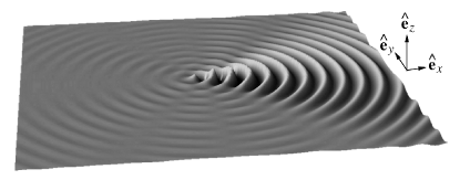
Figure 1: Schematic of the surface elevation of the wave radiated from a line of heaving elements oscillating on otherwise still water. The line has a length of $l/\lambda=2$ and is oscillating in a travelling wave mode with velocity potential given by (31).

For a given amplitude $A_{z}$ and waterplane area $bl$, and since $j_{0}(0)=1$, it can be seen from (31) that in the limit $kr\to\infty$ the ratio of $\phi_{z}$ for a line absorber of length $l$ to that of a point absorber is simply $j_{0}\negmedspace\left(\frac{kl}{2}\left(1-\cos\theta\right)\right)$. Since the surface elevation of the radiated waves is proportional to $\phi_{z}$ at $z=0$, the ratio of the surface elevation of a line absorber to that of a point absorber is also $j_{0}\negmedspace\left(\frac{kl}{2}\left(1-\cos\theta\right)\right)$. Graphs of $j_{0}\negmedspace\left(\frac{kl}{2}\left(1-\cos\theta\right)\right)$ for a point absorber and four line absorbers of different lengths are shown in Figure 2. From this figure it is clear that the point absorber radiates waves in all directions with the same amplitude, whereas the line absorbers radiate at the same amplitude as the point absorber in the $\theta=0$ or $\hat{\mathbf{e}}_{x}$-direction, but they radiate at reduced amplitudes in other directions. Also evident is that the longer the line absorber, the narrower the “beam” of radiated waves and the less the energy radiated.

Figure 2: Plots of the function $j_{0}\negmedspace\left(\frac{kl}{2}\left(1-\cos\theta\right)\right)$. This function describes the $\theta$-dependency of the surface elevation of the radiated waves and that of the velocity potential, $\phi_{z}$, from (31). The $\theta$-dependency plots for a point absorber and four line absorbers of different lengths $l/\lambda$ are shown.

An expression for the full velocity potential, $\phi$, resulting from heave motions and wave diffraction in an incident wave is obtained by substituting the relative motion hypothesis (19) into (13) to give

$$\phi\sim A_{0}\,\varphi_{0}+A_{r}\,\varphi_{z},$$ (32)

where the relative complex amplitude is defined by

$$A_{r}\equiv A_{z}-A_{0}.$$ (33)

Substituting (32) into the integrand in the expression for absorbed power in (12) and expanding gives

$$\phi\,\frac{\partial\bar{\phi}}{\partial n}=\left|A_{0}\right|^{2}\varphi_{0}\,\frac{\partial\bar{\varphi}_{0}}{\partial n}+\bar{A}_{0}A_{r}\varphi_{z}\,\frac{\partial\bar{\varphi}_{0}}{\partial n}\\ +A_{0}\bar{A}_{r}\varphi_{0}\,\frac{\partial\bar{\varphi}_{z}}{\partial n}+\left|A_{r}\right|^{2}\varphi_{z}\,\frac{\partial\bar{\varphi}_{z}}{\partial n}.$$ (34)

The incident wave will contribute no net energy flux through the control surface $S_{C}$, therefore $\iint_{S_{C}}\varphi_{0}\,\partial\bar{\varphi}_{0}/\partial n\,dS=0$. With this observation the term proportional to $\left|A_{0}\right|^{2}$ in (34) can be ignored and the integral in (12) can be written as

$$\iint_{S_{C}}\phi\,\frac{\partial\bar{\phi}}{\partial n}dS=\iint_{S_{C}}\left(A_{0}\bar{A}_{r}\varphi_{0}\,\frac{\partial\bar{\varphi}_{z}}{\partial n}\right.\\ \left.+\bar{A}_{0}A_{r}\varphi_{z}\,\frac{\partial\bar{\varphi}_{0}}{\partial n}+\left|A_{r}\right|^{2}\varphi_{z}\,\frac{\partial\bar{\varphi}_{z}}{\partial n}\right)dS.$$ (35)

The terms on the right-hand side of (35) are evaluated in cylindrical polar coordinates in A. The result shows that $P$ in (12) can be written as

$$P=\frac{\rho}{2}\Im\left\{\left(A_{0}\bar{A}_{r}-\bar{A}_{0}A_{r}\right)c_{g}gk\,bl\right.\\ \left.-i\left|A_{r}\right|^{2}c_{g}gk^{3}\,b^{2}l^{2}\,I(kl)\right\},$$ (36)

where $I(kl)$ is given by

$$I(kl) \equiv\frac{1}{2\pi}\int_{-\pi}^{\pi}j_{0}^{2}\negmedspace\left(\frac{kl}{2}\left(1-\cos\theta\right)\right)\,d\theta,$$ (37)

$$=\frac{4}{3}\cos(kl)\,J_{0}(kl)$$

$$\qquad+\frac{2}{3kl}\left(2kl\sin(kl)-\cos(kl)\right)J_{1}(kl),$$ (38)

and where $J_{0}$ and $J_{1}$ are the zeroth and first-order Bessel functions of the first kind. Since

$$A_{0}\bar{A}_{r}-\bar{A}_{0}A_{r}=2i\Im\left\{A_{0}\bar{A}_{r}\right\},$$

it follows that

$$P=\frac{1}{2}c_{g}\rho\,gk\,bl\left(2\Im\left\{A_{0}\bar{A}_{r}\right\}-\left|A_{r}\right|^{2}k^{2}bl\,I(kl)\right).$$ (39)

In this equation the first term, which can be positive or negative depending on the relative phase of $A_{0}$ and $A_{r}$, gives the energy transferred from the fluid to the body. From the point of view of a near-field perspective, it represents the fluid pressure on the body times the velocity of the body; from the point of view of a far-field perspective, it represents the interference of the incident and radiated waves in the far-field. The second term, which is always negative, gives the power lost due to energy radiated away from the body.

The mean power absorbed by the body, $P$ in (39), is equal to the mean power extracted from the incident wave. The mean power extracted from a wave can be written as the product of the mean energy flux in the wave, denoted by $J$, and the power capture width, denoted by $w$, that is

$$P=w\,J.$$ (40)

The mean energy flux of the plane incident wave described by (14) can be written as

$$J=\frac{1}{2}c_{g}\rho g\left|A_{0}\right|^{2},$$ (41)

where $c_{g}$ is the group velocity given by

$$c_{g}=\frac{d\omega}{dk}=\frac{\omega}{2k}\left(1+\frac{2kh}{\sinh(2kh)}\right).$$ (42)

Substituting (39) and (41) into (40) and rearranging gives the power capture width as

$$w=\frac{2k\,bl}{\left|A_{0}\right|^{2}}\Im\left\{A_{0}\bar{A}_{r}\right\}-k^{3}\,b^{2}l^{2}\frac{\left|A_{r}\right|^{2}}{\left|A_{0}\right|^{2}}I(kl).$$ (43)

This capture width can now be optimised with respect to the phase and amplitude of $A_{r}$. Since the second term on the right-hand side of (43) is positive and independent of phase, to optimise $w$ with respect to phase requires the maximisation of

$$\Im\left\{A_{0}\bar{A}_{r}\right\}=\left|A_{0}\right|\left|A_{r}\right|\sin\psi_{r}$$ (44)

with respect to $\psi_{r}=\arg\left(A_{0}\bar{A}_{r}\right)=\arg\left(A_{0}\right)-\arg\left(A_{r}\right)$, which is the relative phase between $A_{0}$ and $A_{r}$. Maximisation requires that $\sin\psi_{r}=1$, implying that $\psi_{r}=\pi/2$ so that $A_{r}$ lags $A_{0}$ by $\pi/2$ radians and the response velocity (which is proportional to $\partial_{n}\phi_{z}$) is in phase with the excitation force (which is proportional to $\phi_{0}$). Substituting $\psi_{r}=\pi/2$ into (44), and the result into (43), gives

$$w=2k\,bl\frac{\left|A_{0}\right|\left|A_{r}\right|}{\left|A_{0}\right|^{2}}-k^{3}\,b^{2}l^{2}\frac{\left|A_{r}\right|^{2}}{\left|A_{0}\right|^{2}}\,I(kl).$$ (45)

The first term in this equation, which is always positive, accounts for the net power entering the control volume bounded by $S_{C}$ due to the interaction of the incident and radiated waves; the second term, which is always negative, accounts for the energy leaving the control volume due to the radiated waves.

To optimise (45) with respect to the relative amplitude $\left|A_{r}\right|$ consider

$$\frac{dw}{d\left|A_{r}\right|}=2k\,bl\frac{\left|A_{0}\right|}{\left|A_{0}\right|^{2}}-2k^{3}\,b^{2}l^{2}\frac{\left|A_{r}\right|}{\left|A_{0}\right|^{2}}\,I(kl)=0,$$

the solution of which is

$$\left|A_{r}\right|=\frac{1}{k^{2}\,bl\,I(kl)}\left|A_{0}\right|.$$ (46)

Substituting $\left|A_{r}\right|$ from (46) into the first and second terms on the right-hand side of (45) gives the optimal amplitude condition that the radiated power represented by the second term is exactly half of the absorbed power represented by the first term. This, together with the optimal phase condition that $A_{r}$ lags $A_{0}$ by $\pi/2$ radians corresponds to the familiar condition of “impedance matching” to maximise the energy transfer between a source and a load.

The value of $\left|A_{r}\right|$ in (46) is not limited by the volume of the device, and since $k$ is typically relatively small the value of $\left|A_{r}\right|$ can be very large in comparison with $\left|A_{0}\right|$. Because of this, when $\left|A_{r}\right|$ from (46) is substituted back into (45) it gives the optimum capture width for a device of unconstrained motion, or equivalently, unlimited volume, as

$$w=\frac{1}{k\,I(kl)}\quad\mbox{if }\left|A_{r}\right|\mbox{ is unlimited}.$$ (47)

This is identical to the result reported by Farley [6] (see Eq. (18) and the appendix of that work).

In the limit that the length of the line absorber tends to zero, by (69) in A, $\lim_{kl\to 0}I(kl)\to 1$ and therefore $w=1/k$, which agrees with the result obtained for the capture width of an unconstrained heaving point absorbed by, for example, Evans [1] and Newman [3].

At this point a physical interpretation can be given as to why higher capture widths are achievable from line absorbers than from point absorbers: for a line absorber the energy being carried away by radiated waves can be made arbitrarily small while maintaining the amplitude, $\left|A_{r}\right|$, of the radiated wave in the $\theta=0$ direction that is necessary to remove energy from the incident wave by destructive interference. This interpretation is clear from consideration of (45) in the light of (37) and Figure 2. Obviously, to increase the capture width the energy loss given by the second term on the right-hand side of (45) should be minimised while maintaining a high value for the energy absorption given by the first term on the right-hand side. For a point absorber $I(kl)=1$, so $\left|A_{r}\right|$ is the only parameter available that is independent of the incident wave and whose value can be adjusted to maximise $w$. The magnitude of $\left|A_{r}\right|$ needs to be increased to increase the energy absorption from the first term in (45), which is linear in $\left|A_{r}\right|$; but if $\left|A_{r}\right|$ is made too large the energy loss from the second term in (45), which is quadratic in $\left|A_{r}\right|$, dominates. For a line absorber, however, the added degree-of-freedom of length can be used to reduce the spread of the radiated waves, as shown in Figure 2. This reduces the magnitude of $I(kl)$ while keeping a large magnitude for $\left|A_{r}\right|$, so achieving a high energy absorption from the first term on the right-hand side of (45) and a low energy loss from the second.

3.2 Capture width for limited volume

In the preceding section no constraints were placed on the maximum value of the relative amplitude, $\left|A_{r}\right|$, and the maximum capture width for a line absorber of unlimited volume was derived as (47). In this section a motion constraint is placed on $\left|A_{r}\right|$ in (45). In the linear theory presented here such a constraint on $\left|A_{r}\right|$ may be equated to a limit on the maximum swept volume of the device. This constraint may be a consequence of the limited volume of a device, or it may be a consequence of other engineering or control constraints that limit the range of heave motion. Assume for simplicity that the depth, $D$, and the beam, $b$, of each vertically-wall-sided element are independent of its position along the length, $l$, of the line absorber. Here, $D$ is the vertical difference in position between the minimum and maximum submergences of each element of the line absorber. If the element is symmetric about the plane $z=0$ the draft and the freeboard are equal and their sum is equal to $D$. In this case half the maximum swept volume of the line absorber is given by

$$V=bl\,\frac{D}{2},$$

and the maximum value of $\left|A_{r}\right|$ is

$$\max\left(\left|A_{r}\right|\right)=\frac{D}{2}=\frac{V}{bl}.$$ (48)

Substituting $\left|A_{r}\right|$ from (46) into (48) gives the volume limiting condition in terms of $\left|A_{0}\right|$ as

$$\max\left(\left|A_{0}\right|\right)=k^{2}V\,I(kl).$$ (49)

Thus, for a limited volume device the maximum $\left|A_{r}\right|$ is reached when $\left|A_{0}\right|>k^{2}V\,I(kl)$ and the maximum capture width is given by substituting the maximum of $\left|A_{r}\right|$ from (48) into (45). This gives

$$w=\frac{kV}{\left|A_{0}\right|}\left(2-\frac{k^{2}V}{\left|A_{0}\right|}\,I(kl)\right)\\ \quad\mbox{if }\left|A_{0}\right|>k^{2}V\,I(kl).$$

When $\left|A_{0}\right|\leq k^{2}V\,I(kl)$ the optimum capture width is still given by (47). Thus, the maximum capture width of a volume-limited heaving line attenuator can be written as

$$w=\left\{\begin{array}[]{cc}\negthickspace\negthickspace{\displaystyle\frac{1}{k\,I(kl)}},&{\displaystyle\negthickspace\left|A_{0}\right|\leq k^{2}V\,I(kl)},\\ \\ \negthickspace\negthickspace{\displaystyle\frac{kV}{\left|A_{0}\right|}\negthickspace\left(2-\frac{k^{2}V}{\left|A_{0}\right|}\,I(kl)\right)},&{\displaystyle\negthickspace\left|A_{0}\right|>k^{2}V\,I(kl),}\end{array}\right.$$ (50)

where an analytic expression for $I(kl)$ is given by (38).

4 Dimensionless capture width and absorbed power

It is instructive to formulate the results of §3 in dimensionless units. The dimensionless independent variables of device length and device half-swept volume, and the dimensionless dependent variable of capture width, are defined by

$$l^{*} \equiv kl,$$ (51)

$$V^{*} \equiv \frac{k^{2}V}{\left|A_{0}\right|},$$ (52)

$$w^{*} \equiv kw.$$ (53)

Since capture width and absorbed power are related by (40), the definition of $w^{*}$ in (53) suggests a non-dimensional power defined by

$$P^{*}\equiv\frac{k\,P}{J},$$ (54)

where $J$ is given by (41). From (40), (53) and (54) is follows that the dimensionless variables $w^{*}$ and $P^{*}$ are equivalent. Substituting (51)–(53) into (50) gives the dimensionless capture width and power as

$$w^{*}\equiv P^{*}=\left\{\begin{array}[]{cc}\negthickspace{\displaystyle\frac{1}{I\left(l^{*}\right)}},&{\displaystyle V^{*}\,I\left(l^{*}\right)\geq 1,}\\ \\ \negthickspace V^{*}{\displaystyle\left(2-V^{*}\,I\left(l^{*}\right)\right)},&{\displaystyle V^{*}\,I\left(l^{*}\right)<1,}\end{array}\right.$$ (55)

where $I\left(l^{*}\right)=I(kl)$ is the integral given by (38). The forms of the functions $I\left(l^{*}\right)$ and $1/I\left(l^{*}\right)$ are shown in Figure 3. In these plots $l^{*}/2\pi=l/\lambda$ is used as the dimensionless unit on the abscissa as these units correspond to multiples of the wavelength. Shown in the right-hand side plot in Figure 3 is the line $V^{*}=1/I\left(l^{*}\right)$ which marks the boundary between the limited and unlimited volume regimes.

Figure 3: The dimensionless functions $I\left(kl\right)=I\left(l^{*}\right)$ and $V^{*}=1/I\left(l^{*}\right)$.

The point absorber limit is obtained by substituting $\lim_{l^{*}\to 0}I\left(l^{*}\right)\to 1$ into (55) to give

$$\lim_{l^{*}\to 0}w^{*}\to\left\{\begin{array}[]{cc}{\displaystyle 1},&{\displaystyle V^{*}\geq 1,}\\ \\ 2V^{*}{\displaystyle-V^{*2}},&{\displaystyle V^{*}<1.}\end{array}\right.$$ (56)

The term in (56) which applies when ${\displaystyle V^{*}\geq 1}$, that is $w^{*}=1$, is the well known result for the theoretical maximum capture width of a heaving point absorber of unlimited volume. When ${\displaystyle V^{*}\ll 1}$ the term, which is first-order in volume, dominates and the capture width can be written as $w^{*}=2V^{*}$, or, equivalently, $P^{*}/V^{*}=2$. This corresponds to Budal’s upper bound on the maximum capture width, or power per unit volume, of a finite-volume heaving point absorber [see 11]. The term that is second-order in volume is a modification arising from the inclusion of energy loss due to radiated waves.

The infinite length line absorber limit is obtained by substituting $\lim_{l^{*}\to\infty}I\left(l^{*}\right)\to 0$ into (55) to give

$$\lim_{l^{*}\to\infty}w^{*}\to 2V^{*}\quad\mbox{for all }V^{*}.$$ (57)

This can also be written as $P^{*}/V^{*}=2$ for all $V^{*}$. Comparing (56) and (57) shows that for a heaving point absorber the maximum capture width is limited to $w^{*}=1$, no matter how great the volume; for a line absorber in the limit infinite length, however, the maximum capture width scales linearly with volume, that is $w^{*}=2V^{*}$.

Plots of dimensionless capture width (or absorbed power) from (55) are shown in Figure 4. The two plots give different illustrations of the effect on $w^{*}$ of changing the volume and length of a device. The solid line in the left-hand plot in Figure 4 shows that increasing volume above $V^{*}=1$ gives no increase in $w^{*}$ for a point absorber; the dashed lines show that, for line absorbers, increasing $V^{*}$ above $1$ can increase $w^{*}$, and that the increase is greater for a longer device. In fact, the dotted line marks where $w^{*}=2V^{*}$ which shows that the maximum dimensionless capture widths for an infinite length line absorber is equal to its dimensionless swept volume. The fine dotted line marks where $w^{*}=V^{*}$ which is the line of transition between the unlimited volume regime below the line and the limited volume regime above it. It is clear from this plot that the minimum half-swept volume required for a point absorber to achieve its maximum capture width is $V^{*}=1$, and for a line absorber it is $V^{*}=w^{*}$. Note that $V^{*}=1$ is equivalent to $V/\lambda^{2}\left|A_{0}\right|=1/4\pi^{2}\approx 0.025$, which aids in interpreting the dimensionless volume as it states that the minimum half-swept volume for a point absorber to achieve its maximum capture width is about $2.5\%$ of the natural measure of volume given by the square of the wavelength times the amplitude of the wave, that is, $\lambda^{2}\left|A_{0}\right|$.

The right-hand plot in Figure 4 shows the gains in $w^{*}$ that can be achieved by “stretching out” different fixed-volume point absorbers to line absorbers of different lengths. The points where the lines terminate at $l^{*}=0$ represent the dimensionless capture widths of point absorbers of the appropriate volumes. There is little difference in $w^{*}$ between point and line absorbers when $V^{*}<0.5$, that is, well within the volume-limited regime of the point absorber. For the unlimited volume regime of $V^{*}\geq 1$ the capture width of the point absorber is at its theoretical maximum of $w^{*}=1$ and the lines for $V^{*}=1$, $2$ and $4$ all converge to $w^{*}=1$ as $l^{*}\to 0$. For finite length line absorbers, however, significant increases in capture width are achievable above $w^{*}=1$, as shown in the figure and in the examples given in Table 1.

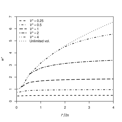
Figure 4: Dimensionless capture width, $w^{*}$, from (55) as a function of dimensionless half-swept volume, $V^{*}$, and dimensionless device length, $l^{*}$.

half-swept	length,	capture-
volume, $V^{*}$	$l^{*}/2\pi=l/\lambda$	width, $w^{*}$
1	0	1
1	1	1.684
1	2	1.782
2	0	1
2	1	2.735
2	2	3.127
3	0	1
3	1	3.154
3	2	4.036
unlimited	0	1
unlimited	1	3.162
unlimited	2	4.583

Table 1: Examples of maximum dimensionless capture widths for different dimensionless volumes and lengths.

Plots of dimensionless absorbed powers (or capture widths) per unit dimensionless volume are shown in Figure 5. In the left-hand plot in Figure 5 the fine dotted line marks the line of $P^{*}/V^{*}=1$, which is the line of transition between the limited volume regime above the line and unlimited volume regime below it. In this plot the limited-volume dimensionless powers converge to $P^{*}/V^{*}=2$ at $V^{*}=0$ for all device lengths $l^{*}$. This maximum value of $P^{*}/V^{*}=2$ corresponds to Budal’s upper bound expressed in the dimensional units of (51)–(54). Budal’s upper bound applies to all wave energy absorbers, however, point absorbers can only reach Budal’s upper bound in the zero-volume limit, whereas line absorber in the infinite-length limit can reach Budal’s upper bound for any volume. This is evident from the infinite-length limit of (55) giving $P^{*}/V^{*}=2$ which is independent of volume. From the left-hand plot in Figure 5 it is clear that for small volume devices there is no significant advantage to using an attenuating line absorber compared to a point absorber. For larger volume devices, however, the same plot shows how the power per unit volume decreases less rapidly for a line absorber than for an equivalent volume point absorber, and the rate of decrease of power per unit volume is less for longer line absorbers (being zero in the limit of an infinitely long line absorber). In fact, by dividing volume of a single point absorber with $V^{*}=1$ into ever smaller volume point absorbers the maximum power per unit volume that can be achieved goes from $P^{*}/V^{*}=1$ to $P^{*}/V^{*}=2$ and, therefore, the maximum absorbed power is doubled. This severe drop-off in $P^{*}/V^{*}$ with increasing $V^{*}$ for point absorbers is an illustration of the “small is beautiful” argument made by Falnes [11].

The right-hand plot in Figure 5 gives an alternative illustration of how, if efficiency is measured in terms of absorbed power per unit volume, for all device lengths, $l^{*}$, devices of smaller volume always have greater efficiencies. Note that in this plot the dotted line starting at $l^{*}=0$ and $P^{*}/V^{*}=2$ represents the power per unit volume in the unlimited volume regime for the case $V^{*}=0.5$. The corresponding line for $V^{*}=0.25$ is off the scale.

Figure 5: Dimensionless power per unit dimensionless volume, $P^{*}/V^{*}$, from (55) as a function of dimensionless half-swept volume, $V^{*}$, and dimensionless device length, $l^{*}$.

5 Application to realistically sized WECs

half-swept
volume,	length,
$V$ (m3)	$l$ (m)	WEC of similar size
240	0	OPT PB150 [12]
940	0	WaveBob [13]
350	120	Pelamis FSP [14]
790	180	Pelamis P2 [15]
1700	210	possible future Pelamis

Table 2: Selection of WEC sizes chosen to represent realistic production sizes based on estimates of the sizes of devices already built or recently proposed.

The advantage of formulating the results in dimensionless units is that the number of independent variables is reduced from four ($k$, $l$, $V$, and $\left|A_{0}\right|$) to just two ($l^{*}$ and $V^{*}$). In dimensionless units, however, it is not immediately obvious where a particular incident wave and WEC combination will occur on the graphs. In this section we consider the five realistically sized WECs described in Table 2. It is stressed that the results in the following figures are not representative of the actual capture widths or absorbed powers of these devices, but only that devices of these approximate volumes and lengths have already been built or may be built in the near future.

Figure 6: Dimensionless capture width, $w^{*}$, from (55) as a function of dimensionless half-swept volume, $V^{*}$, for WECs in Table 2 operating in four different incident wave defined by their $(H,T)$.

Figure 7: Absorbed power, $P$, from (55) as a function of half-swept volume, $V$, for WECs with sizes described in Table 2 operating in four different $(H,T)$ incident waves.

Figure 6 shows the points of maximum dimensionless capture width plotted against dimensionless volume for the sizes of WECs given in Table 2 operating in the four incident waves with $(H,T)$ equal to $(2\mbox{m},8\mbox{s})$, $(2\mbox{m},10\mbox{s})$, $(3\mbox{m},8\mbox{s})$ and $(3\mbox{m},10\mbox{s})$. These four incident waves broadly correspond to those that would occur close to the centres of the available energy resource when weighted by annual average occurrence. They have incident power in ratios of $1,$ $1.25$, $2.25$ and $2.81$ respectively. Also, shown in Figure 6 are contours of constant dimensionless length. The set of four plots show how the dimensionless volume and maximum capture width of a particular WEC depends on the wave height and period of the incident wave. The plots show that the largest volume point absorber appears below the line $w^{*}=V^{*}$ and is, therefore, operating in its unlimited volume regime and unnecessarily large for all but the $(3\mbox{m},10\mbox{s})$ incident wave. The largest volume line-absorber, however, is only unnecessarily large for the $(2\mbox{m},8\mbox{s})$ incident wave, even though it is nearly twice the volume of the largest point absorber. The smallest point absorber has its maximum capture width limited by its small volume in all but the $(2\mbox{m},8\mbox{s})$ incident wave. The mid-sized line absorber has less volume than the large point absorber, yet its maximum capture width is about four times larger in the $(2\mbox{m},8\mbox{s})$ wave, three times larger in the $(3\mbox{m},8\mbox{s})$ wave, twice as large in the $(2\mbox{m},10\mbox{s})$ wave, and one and half times as large in the $(3\mbox{m},10\mbox{s})$ wave. For further clarity, Figure 7 shows points of dimensional maximum absorbed power plotted against dimensional volume for the size of WECs given in Table 2 operating in the four incident waves as used in Figure 6. A set of conveniently spaced contours of constant length are also shown in these plots. This set of four plots shows how the maximum absorbed power of a particular size of WEC depends on the wave height and period of the incident wave.

6 Conclusions

The theoretical maximum absorbed power and capture width of a limited volume attenuating line absorber heaving in a travelling wave mode in the presence of progressive regular incident wave has been derived in the frequency domain using the linearised theory of the interaction of water waves and structures. The results are presented in dimensionless form which has the advantage of reducing the number of dependent variables from four to just two: dimensionless length, $l^{*}$, and dimensionless half-swept volume, $V^{*}$. In the zero-length limit the results for the limited volume line absorber reduce to those for a point absorber; and in the zero-volume limit they reduce to the result expressed by Budal’s upper bound. It is shown that, in dimensionless units, the maximum dimensionless capture width of a point absorber is $w^{*}=1$ and that the smallest volume required to achieve this capture width is $V^{*}=1$. The dimensionless capture width and volume both depend on the incident wave: a value of $w^{*}=1$ corresponds to a width of about $16\%$ of the wavelength; a value of $V^{*}=1$ corresponds to about $2.5\%$ of the rectangular volume given by the square of the wavelength times the wave amplitude. Increasing the volume of a point absorber beyond $V^{*}=1$ gives no increase in capture width. For an attenuating line absorber, however, in the limit of infinite length the maximum capture width is $w^{*}=2V^{*}$. Thus, there is no limit to the capture width of a line absorber provided it has sufficient volume and length. It is shown that a particular fixed-length line absorber will have a maximum capture width of $w^{*}>1$ and that the smallest volume required to achieve this capture width is $V^{*}=w^{*}$ .

This has profound implications for the economics of power generation from wave energy converters. Even though small volume point absorbers are more efficient than larger volume point absorbers in terms of power absorbed per unit swept-volume of device, engineering limitations make installation and operation of very large numbers of very small devices excessively costly and uneconomic. A point absorber has a limit on its capture width and usable volume, whereas, in theory, line absorbers can be indefinitely scaled-up in volume and length to give unlimited capture widths. This theoretical advantage of line absorbers over point absorbers applies to realistically sized wave energy converters currently in operation. Thus, line absorbers can be progressively scaled-up in volume and length to give increasingly large capture widths while retaining dimensions compatible with cost-effective engineering. For example, a line absorber with a volume equal to the maximum usable volume of a point absorber and a length equal to twice the wavelength of the incident wave can absorb nearly $80\%$ more power than a point absorber of the same volume. Doubling this line absorber’s volume gives over three times the absorbed power of the point absorber, and tripling it gives over four times the absorbed power. Thus, it is clear that by installing fewer larger line absorbers valuable economies of scale can be achieved from line absorbers that are not achievable from point absorbers.

Appendix A Integrals by the method of stationary phase

The terms on the right-hand side of (35) are evaluated in cylindrical polar coordinates as follows. Substituting $x=r\cos\theta$ into (14), $\varphi_{0}$ is written as

$$\varphi_{0}=-i\frac{g}{\omega}\frac{\cosh(k(z+h))}{\cosh(kh)}\mathrm{e}^{ikr\cos\theta}.$$ (58)

Also, using (14) along with $n_{x}=\cos\theta$ and $n_{z}=0$ on the control surface $S_{C}$, and the observation that $\bar{\varphi}_{0}$ is not a function of $y$, it follows that

$$\frac{\partial\bar{\varphi}_{0}}{\partial n}=\frac{gk}{\omega}\frac{\cosh(k(z+h))}{\cosh(kh)}\,\cos\theta\,\mathrm{e}^{-ikr\cos\theta},\\ \quad\mbox{on }S_{C}.$$ (59)

Next, using

$$\mathbf{n}=\hat{\mathbf{e}}_{r}\quad\mbox{on }S_{C},$$

and the gradient operator in cylindrical coordinates

$$\bm{\nabla}=\hat{\mathbf{e}}_{r}\frac{\partial}{\partial r}+\hat{\mathbf{e}}_{\theta}\frac{1}{r}\frac{\partial}{\partial\theta}+\hat{\mathbf{e}}_{z}\frac{\partial}{\partial z},$$

it follows that

$$\mathbf{n}\cdot\bm{\nabla}\bar{\varphi}_{z}=\frac{\partial\bar{\varphi}_{z}}{\partial n}\equiv\frac{\partial\bar{\varphi}_{z}}{\partial r}\quad\mbox{on }S_{C}.$$

Evaluating $\partial\bar{\varphi}_{z}/\partial n$ by differentiating (31) with respect to $r$, it can be shown that

$$\frac{\partial\bar{\varphi}_{z}}{\partial n} \sim\frac{igk^{3}bl}{\omega\left(2\pi kr\right)^{1/2}}\frac{\cosh(k(z+h))}{\cosh(kh)}\times$$

$$j_{0}\negmedspace\left(\frac{kl}{2}\left(1-\cos\theta\right)\right)\,\mathrm{e}^{-ikr+i\pi/4}\quad\mbox{on }S_{C},$$ (60)

where $j_{0}$ is the zeroth spherical Bessel function of the first kind and, since $kr\to\infty$ on $S_{C}$, only the highest order terms in $kr$ have been retained.

Combining (31), (58), (59) and (60), the three integrands on the right-hand side of (35) can now be simplified and written as

$$\varphi_{0}\,\frac{\partial\bar{\varphi}_{z}}{\partial n} \sim\frac{g^{2}k^{3}bl}{\omega^{2}\left(2\pi kr\right)^{1/2}}\left(\frac{\cosh(k(z+h))}{\cosh(kh)}\right)^{2}\times$$

$$j_{0}\negmedspace\left(\frac{kl}{2}\left(1-\cos\theta\right)\right)\,\mathrm{e}^{-ikr\left(1-\cos\theta\right)+i\pi/4},$$ (61)

$$\varphi_{z}\,\frac{\partial\bar{\varphi}_{0}}{\partial n} \sim-\frac{g^{2}k^{3}bl}{\omega^{2}\left(2\pi kr\right)^{1/2}}\left(\frac{\cosh(k(z+h))}{\cosh(kh)}\right)^{2}\times$$

$$\cos\theta\,j_{0}\negmedspace\left(\frac{kl}{2}\left(1-\cos\theta\right)\right)\,\mathrm{e}^{ikr\left(1-\cos\theta\right)-i\pi/4},$$ (62)

$$\varphi_{z}\,\frac{\partial\bar{\varphi}_{z}}{\partial n} \sim-\frac{ik}{2\pi kr}\left(\frac{gk^{2}bl}{\omega}\,\frac{\cosh(k(z+h))}{\cosh(kh)}\right)^{2}\times$$

$$j_{0}^{2}\negmedspace\left(\frac{kl}{2}\left(1-\cos\theta\right)\right).$$ (63)

In cylindrical polar coordinates the integral over $S_{C}$ on the left-hand of (35) is expressed as

$$\iint_{S_{C}}\phi\,\frac{\partial\bar{\phi}}{\partial n}\,dS=\int_{-h}^{0}\int_{-\pi}^{\pi}\phi\,\frac{\partial\bar{\phi}}{\partial n}\,r\,d\theta\,dz.$$ (64)

Each of (61)–(63) has the same $z$-dependency. Integrating out this $z$-dependency gives, after simplification and substitution of the dispersion relationship from (15),

$$\int_{-h}^{0}\frac{\cosh^{2}(k(z+h))}{\cosh^{2}(kh)}\,dz=\frac{\omega c_{g}}{gk},$$ (65)

where $c_{g}$ is the group velocity given by (42). The integrals over $\theta$ of (61)–(63) are evaluated using the method of stationary phase, which states that for real-valued smooth functions $f$ and $g$, when $f^{\prime}(\theta_{0})=0$ and $K\to\infty$,

$$\int_{-\infty}^{\infty}g(\theta)\,\mathrm{e}^{iKf(\theta)}\,d\theta\\ \sim g(\theta_{0})\sqrt{\frac{2\pi}{Kf^{\prime\prime}(\theta_{0})}}\mathrm{e}^{i\left(Kf(\theta_{0})+\pi/4\right)},\\ \mbox{with }f^{\prime}(\theta_{0})=0,\,K\to\infty.$$ (66)

Substituting $K=kr$, $g(x)=j_{0}\negmedspace\left(\frac{kl}{2}\left(1-\cos\theta\right)\right)$, $f(x)=\cos\theta-1$ and $\theta_{0}=0$ into (66) gives the integral of (61) over $\theta$ as

$$\int_{-\pi}^{\pi}j_{0}\negmedspace\left(\frac{kl}{2}\left(1-\cos\theta\right)\right)\,\mathrm{e}^{-ikr(1-\cos\theta)}\,d\theta\\ \sim\sqrt{\frac{2\pi}{kr}}\mathrm{e}^{-i\pi/4}.$$ (67)

Substituting $K=kr$, $g(x)=\cos\theta\,j_{0}\negmedspace\left(\frac{kl}{2}\left(1-\cos\theta\right)\right)$, $f(x)=1-\cos\theta$, and $\theta_{0}=0$ into (66) gives the integral over $\theta$ of (62) as

$$\int_{-\pi}^{\pi}\cos\theta\,j_{0}\negmedspace\left(\frac{kl}{2}\left(1-\cos\theta\right)\right)\mathrm{e}^{ikr(1-\cos\theta)}\,d\theta\\ \sim\sqrt{\frac{2\pi}{kr}}\mathrm{e}^{i\pi/4}.$$ (68)

For convenience of notation the integral of (63) over $\theta$ is denoted by $I(kl)$ as defined by the integral in (37). As stated by Farley [6, Eq. (20)], $I(kl)$ can be expressed analytically as in (38) in terms of first-order Bessel functions of the first kind, $J_{0}$ and $J_{1}$. Since the $kl\to 0$ limits of the Bessel functions are

$$\lim_{kl\to 0}J_{0}(kl) = 1,$$

$$\lim_{kl\to 0}\frac{J_{1}(kl)}{kl} = \frac{1}{2},$$

the $kl\to 0$ limit of (38) is

$$\lim_{kl\to 0}I(kl)\to 1.$$ (69)

Equations (65), (67), (68) and (37) are now used, along with (64), to evaluate the integrals of (61)–(63) over $S_{C}$. The results are

$$\int_{-h}^{0}\int_{-\pi}^{\pi}\varphi_{0}\,\frac{\partial\bar{\varphi}_{z}}{\partial n}\,r\,d\theta\,dz \sim\frac{c_{g}gkbl}{\omega},$$

$$\int_{-h}^{0}\int_{-\pi}^{\pi}\varphi_{z}\,\frac{\partial\bar{\varphi}_{0}}{\partial n}\,r\,d\theta\,dz \sim-\frac{c_{g}gkbl}{\omega},$$

$$\int_{-h}^{0}\int_{-\pi}^{\pi}\varphi_{z}\,\frac{\partial\bar{\varphi}_{z}}{\partial n}\,r\,d\theta\,dz \sim-\frac{ic_{g}gk^{3}b^{2}l^{2}}{\omega}\,I(kl).$$

Substituting these expressions into (35) and the result into (12) gives (36).

References

- Evans [1976] D. V. Evans, A theory for wave-power absorption by oscillating bodies, Journal of Fluid Mechanics 77 (1976) 1–25.
- Mei [1976] C. C. Mei, Power extraction from water waves, Journal of Ship Research 20 (2) (1976) 63–66.
- Newman [1976] J. N. Newman, The Interaction of Stationary Vessels with Regular Waves, in: Proceedings of the 11th Symposium on Naval Hydrodynamics, Mechanical Engineering Publications Limited, London, UK, 491–501, 1976.
- Evans [1981] D. V. Evans, Maximum wave-power absorption under motion constraints, Applied Ocean Research 3 (1981) 200.
- Pizer [1993] D. J. Pizer, Maximum wave-power absorption of point absorbers under motion constraints, Applied Ocean Research 15 (1993) 227–234.
- Farley [1982] F. J. M. Farley, Wave energy conversion by flexible resonant rafts, Applied Ocean Research 4 (1) (1982) 57–63.
- Newman [1979] J. N. Newman, Absorption of wave energy by elongated bodies, Applied Ocean Research 4 (1979) 189–196.
- Rainey [2001] R. C. T. Rainey, The Pelamis wave energy converter: it may be jolly good in practice, but will it work in theory?, in: Proceedings of the 16th International Workshop on Water Waves and Floating Bodies, Hiroshima, Japan, 1–6, 2001.
- Mei [1989] C. C. Mei, The applied dynamics of ocean surface waves, Wiley-Interscience, John Wiley & Sons, Inc., iSBN 0-471-06407-6, 1989.
- McIver [1994] P. McIver, Low-frequency asymptotics of hydrodynamic forces on fixed and floating structures, in: M. Rahman (Ed.), Waves Engineering, Computational Mechanics Publications, 1–49, 1994.
- Falnes [1993] J. Falnes, Small is beautiful: How to make wave energy economic, in: European wave energy symposium, Edinburgh, Scotland, 367–372, 1993.
- Inc. [2011] O. P. T. Inc., URL http://www.oceanpowertechnologies.com/pb150.htm, a 50% submerged torus of about diameter 11m and height 2.5m, 2011.
- Ltd. [2011] W. Ltd., URL http://wavebob.com/key-features/, a 50% submerged torus of about diameter 20m and height 8m, 2011.
- Pelamis Wave Power Ltd. [2011a] Pelamis Wave Power Ltd., URL http://www.pelamiswave.com/our-technology/development-history%, a 30% submerged line absorber of length 120m and diameter 3.5m, 2011a.
- Pelamis Wave Power Ltd. [2011b] Pelamis Wave Power Ltd., URL http://www.pelamiswave.com/our-technology/the-p2-pelamis, a 35% submerged line absorber of length 180m and diameter 4m, 2011b.