Uncertainty Relations in Statistical Mechanics: a numerical study in small lattice systems

Abstract

We have analyzed the validity of uncertainty relations between the fluctuations of thermodynamically conjugated extensive and intensive variables within the field of statistical mechanics. Analysis is presented for two particular examples of small lattice systems that are in contact with reservoirs of comparable sizes: an Ising paramagnet and an Ising ferromagnet. The numerical results enable determination of the range of applicablity of the proposed relations. Due to the fact that the examples correspond to systems described by discrete variables, the uncertainty relations are not valid if the probability of boundary states is too high.

I Introduction

Uncertainty relations can be established in any physical theory involving random conjugated variables characterized by probability distribution functions. The present paper deals with uncertainty relations in statistical mechanics.

Statistical mechanics combines equilibrium thermodynamics with a probability postulate TerHaar1955 ; Huang1987 . Following the standard Gibbs ensemble theory, in the microcanonical ensemble it is assumed that all mechanical variables are constrained to a fixed value (or are allowed to vary within a fixed small range), while their entropy-conjugated variables are free to fluctuate. Other ensembles (Canonical, Grand-Canonical, …) are introduced by relaxing the constraint on one or more mechanical variables. This is done by assuming that these mechanical variables can be exchanged with a reservoir, which is defined as a macroscopic body of dimensions much larger than those of the system. The exchange is supposed to be controlled by parameters (which are characteristic of the reservoir) that are identified as intensive variables. Formally, the change of variables when passing from the microcanonical to other ensembles is undertaken via Legendre transforms. In the spirit of equilibrium thermodynamics, the intensive variables are assumed to have the same value both in the reservoir and in the system and are usually treated as non-fluctuating variables. Therefore, within this basic framework, uncertainty relations are not expected to apply Kittel1988 .

While it seems reasonable that intensive variables of a very large reservoir (a system characterized by large amounts of mechanical variables ) are treated as non-fluctuating variables, there is no reason for such an assumption when dealing with intensive variables corresponding to a small reservoir or system. Therefore, we will adopt the point of view that, in general, for a system in contact with a reservoir (regardless of size) fluctuations of intensive variables should occur in the system induced by the fluctuations of the corresponding conjugated mechanical variables. From this point of view, uncertainty relations are expected to play an important role for a correct understanding of the behaviour of equilibrium fluctuations of thermodynamic variables, with consequences in the experimental measurements of these variables. Actually this simple picture has received some experimental support Chui1992 and thus it is reasonable to ask whether or not uncertainty relations can be formulated and what their applicability limits are.

The problem was already discussed by Bohr and Heisenberg as soon as Heisenberg proposed the uncertainty principle in quantum mechanics Bohr . Therefore, during the last century a number of papers were published dealing with this problem. An interesting article where these issues have been reviewed is the paper by Uffink and van Lith Uffink1999 . More recently, Velázquez and Curilef Velasquez2009 revisited the problem within the framework discussed some years before by Mandelbrot Mandelbrot1962 , Gilmore Gilmore1985 and others. The vast majority of these works have been formulated from a purely theoretical point of view, and applications to particular examples (analytical or numerical) are scarce. The aim of the present paper is to numerically analyze the validity of uncertainty relations in two simple lattice models and shed some light on controversial interpretations Mandelbrot1962 ; Kittel1988 ; Kittel1989

The paper is organized as follows. In section II we summarize a derivation of the uncertainty relations in statistical mechanics. In section III we numerically analyze two examples corresponding to an Ising paramagnet and an Ising ferromagnet. Finally, in Section IV we discuss the relevance of the results in relation to temperature measurements in small thermodynamic systems and draw some conclusions.

II Uncertainty relations in statistical mechanics

II.1 Fluctuations in continuous probability distributions

Following the mathematical treatment proposed in Ref. Velasquez2009, , let us consider a continuous probability distribution, $p\left(\bf{x}\right)d\bf{x}$, defined within the domain $\Omega\in\Re^{n}$, which is assumed to vanish at the boundary $\partial\Omega$. The average value of the derivative of any analytical function $f\left(\bf{x}\right)$ with respect to one of the components of $\bf{x}$, can be expressed as:

$$\begin{split}\left\langle\frac{\partial f}{\partial x_{i}}\right\rangle=\underset{\Omega}{\int}d^{n}xp\left(\bf{x}\right)\frac{\partial f\left(\bf{x}\right)}{\partial x_{i}}=\underset{\Omega}{\int}d^{n}x\left(\frac{\partial}{\partial x_{i}}\left(p\left(\bf{x}\right)f\left(\bf{x}\right)\right)-f\left(\bf{x}\right)\frac{\partial p\left(\bf{x}\right)}{\partial x_{i}}\right)=\\ =-\underset{\Omega}{\int}d^{n}xp\left(\bf{x}\right)f\left(\bf{x}\right)\frac{1}{p\left(\bf{x}\right)}\frac{\partial p\left(\bf{x}\right)}{\partial x_{i}}\equiv\left\langle f\left(\bf{x}\right)\Gamma_{i}\left(\bf{x}\right)\right\rangle\ \end{split}$$ (1)

where we have defined the affinities:

$$\Gamma_{i}\left(\bf{x}\right)\equiv-\frac{1}{p(\bf{x})}\frac{\partial p\left(\bf{x}\right)}{\partial x_{i}}=-\frac{\partial\ln p\left(\bf{x}\right)}{\partial x_{i}}\;.$$ (2)

Two interesting particular cases of the result in (1) can be obtained by choosing $f\left(\bf{x}\right)=1$ and $f\left(\bf{x}\right)=x_{j}$. In the first case one gets

$$\left\langle\Gamma_{i}\right\rangle=0\;\;\forall i,$$ (3)

and in the second case

$$\left\langle x_{j}\Gamma_{i}\right\rangle=\delta_{ij}.$$ (4)

Let us now define the differences:

$$\Delta x_{j}\equiv x_{j}-\left\langle x_{j}\right\rangle\;,$$ (5)

$$\Delta\Gamma_{i}\equiv\Gamma_{i}-\left\langle\Gamma_{i}\right\rangle\;.$$ (6)

The variances $\left\langle(\Delta A)^{2}\right\rangle$ and the covariances $\left\langle\Delta A\Delta B\right\rangle$ of arbitrary differences $\Delta A$ and $\Delta B$ can be interpreted as a scalar products in a vectorial space where the metric is given by the probability distribution. In particular, the square root of the variance $\sqrt{\langle\left(\Delta A\right)^{2}\rangle}$ of a random variable $A$ (which we will denote as the fluctuation of $A$) is the norm of the vector $\Delta A$ in this metric. Therefore, in our case, taking into account the Schwartz inequality, we can write:

$$\sqrt{\left\langle\left(\Delta x_{j}\right)^{2}\right\rangle\left\langle\left(\Delta\Gamma_{i}\right)^{2}\right\rangle}\geq\left\langle\Delta x_{j}\Delta\Gamma_{i}\right\rangle\;.$$ (7)

From (3) and (4), the right-hand-side term can be expressed as:

$$\left\langle\Delta x_{j}\Delta\Gamma_{i}\right\rangle=\left\langle x_{j}\Gamma_{i}\right\rangle-\left\langle x_{j}\right\rangle\left\langle\Gamma_{i}\right\rangle=\delta_{ij}\;.$$ (8)

Thus, we obtain an inequality relating the variances of the variable $x_{i}$ and the affinity $\Gamma_{j}$:

$$\sqrt{\left\langle\left(\Delta x_{j}\right)^{2}\right\rangle\left\langle\left(\Delta\Gamma_{i}\right)^{2}\right\rangle}\geq\delta_{ij}\;.$$ (9)

It is worth noting that other authors have used different mathematical approaches Gilmore1985 ; Uffink1999 ; Falcini2011 to treat this problem.

II.2 Application to Statistical Mechanics:

In this subsection we will discuss how to apply the results obtained above in order to establish uncertainty relations in statistical mechanics. Actually, the key point will be to find a convenient definition of the set $\Omega$, the probabilities $p({\bf x})$ and the affinities $\Gamma_{i}$.

We proceed by dividing an isolated universe into two interacting parts that can exchange one or more mechanical variables. One part (usually the smallest one, which we wish to study) will be called the ”system”, while the other part will be the ”reservoir”. For the closed universe we assume Boltzmann equiprobability and therefore its entropy will be given by:

$${\cal S}/k=\ln{W}\;,$$ (10)

where $W$ is the total number of microstates of the universe and $k$ is the Boltzmann constant.

Let us consider the set $\Omega$ of mechanical variables describing the system ${\bf X}=(X_{1},X_{2},\cdots X_{n})$. The corresponding variables for the universe ${\bf X}^{U}$ are constant (closed). Therefore, for the reservoir we have ${\bf X}^{R}={\bf X}^{U}-{\bf X}$. From knowledge of the number of microstates of the universe $W({\bf X})$ for which the system variables take values within $({\bf X},{\bf X}+d{\bf X})$ we can determine the probability density:

$$p\left({\bf X}\right)d{\bf X}=\frac{W\left(\bf{X}\right)d\bf{X}}{W\Omega_{0}}\;,$$ (11)

where $\Omega_{0}$ is an elementary volume in $\Omega$ that will be irrelevant for further developments. It is introduced here in order to have consistent units. Assuming that this probability density $p({\bf X})$ is a finite function, Eq. (11) can be written in terms of a universe dimensionless entropy which depends on the system variables:

$$S^{U}\left(\bf{X}\right)\equiv\ln\left[W\left(\bf{X}\right)\right]$$ (12)

Therefore we have

$$p\left({\bf X}\right)d{\bf X}=\frac{e^{S^{U}\left({\bf X}\right)}d{\bf X}}{W\Omega_{0}}\;,$$ (13)

which is none other than Einstein’s formula for fluctuations Einstein1 ; Einstein2 . At this point, without making any assumptions about the separability of the function $S^{U}\left({\bf X}\right)$, we can define the affinities between the system and reservoir as the partial derivative:

$$\Gamma_{i}=-\frac{\partial S^{U}\left({\bf X}\right)}{\partial X_{i}}\;.$$ (14)

Note that $\Gamma_{i}$ has units inverse of those of $X_{i}$ since $S^{U}$ is dimensionless. In some cases, it can be assumed that $S^{U}\left({\bf X}\right)$ can be split into a part related to the entropy of the studied system, $S$, and a part related to the reservoir, $S^{R}$, so that

$$S^{U}\left({\bf X}\right)=S\left({\bf X}\right)+S^{R}\left({\bf X}^{U}-{\bf X}\right)\,.$$ (15)

Since functions $S$ and $S^{R}$ only depend on the internal structure of the corresponding parts, it then seems natural to define intensive variables for the system and reservoir in analogy with thermodynamics:

$$\gamma_{i} = \frac{\partial S\left({\bf X}\right)}{\partial X_{i}}$$

$$\gamma^{R}_{i} = \frac{\partial S^{R}\left({\bf X}^{U}-{\bf X}\right)}{\partial\left(X^{U}_{i}-X_{i}\right)}\;.$$ (16)

Therefore, assuming separability, the affinity can be expressed as:

$$\Gamma_{i}=\gamma_{i}^{R}-\gamma_{i}\;.$$ (17)

The results derived in subsection II.1 can now be written in terms of the preceding definitions. Without assuming separability, from Eq. (3) we get:

$$\left\langle\Gamma_{i}\right\rangle=0\;,$$ (18)

and from the inequality relation in (9), we can write:

$$\sqrt{\left\langle\left(\Delta X_{j}\right)^{2}\right\rangle\left\langle\Gamma_{i}^{2}\right\rangle}\geq\delta_{ij}\;.$$ (19)

When separability holds, equations (18) and (19)become

$$\left\langle\gamma_{i}^{R}-\gamma_{i}\right\rangle=0\$$ (20)

and

$$\sqrt{\left\langle\left(\Delta X_{j}\right)^{2}\right\rangle\left\langle\left(\gamma_{i}^{R}-\gamma_{i}\right)^{2}\right\rangle}\geq\delta_{ij}\;,$$ (21)

respectively. These are the main results that we will numerically test in the examples in section III. Note that for the particular case of choosing energy as a mechanical variable, in the separable case, the above two equations read:

$$\left\langle\beta^{R}-\beta\right\rangle=0$$ (22)

and

$$\sqrt{\left\langle\Delta E^{2}\right\rangle\left\langle\left(\beta^{R}-\beta\right)^{2}\right\rangle}\geq 1\;,$$ (23)

where we have used the more common symbols $\beta$ and $\beta^{R}$ to represent the intensive variables conjugated for the energy of the system and reservoir.

Equations (18), (20) or (22) are essentially probabilistic versions of the Zero-th Principle of Thermodynamics Redlich1970 . Because of the fluctuations of the system and reservoir, the equilibrium conditions are not an absolute equality, but only apply to statistical averages of the intensive variables. It is important to note that with the separability assumption the conjugated variables of a system appear as functions of extensive variables of the same system (as in thermodynamics) and that the same happens when the roles of the system and reservoir are interchanged.

Equations (19), (21) or (23) state that fluctuations in conjugated thermodynamic variables are related in a form which is similar to the uncertainty relations in quantum mechanics. These results are usually referred to as uncertainty relations in statistical physics and, even though their interpretation in quantum mechanics is different, they both come from the same mathematical base, as noted in Ref.  Gilmore1985, .

At this point it is convenient to point out that the previous results were obtained after neglecting the contribution from the boundary $\partial\Omega$ in Eq. (1) and after considering a continuous character for the variables $X_{i}$ describing the system. Therefore, the uncertainty relation (19) and the equilibrium condition (18) may not hold if states with extreme values of the variables $X_{i}$ (at the boundary $\partial\Omega$) are likely to occur. Such states will be called boundary states and in the following examples, that have a discrete character, it will be important to evaluate their probability and check under which circumstances they become too high.

II.3 First-order approximation

Let us consider a universe in which the dimensionless entropy $S^{U}$ can be separated between the system and reservoir and we focus only on the energy of the system $E$ as a mechanical variable. Let us assume that $S^{U}$ or equivalently, the continuous probability density $p\left(E\right)dE$, is centred about a maximum at $E^{eq}$. We also require that the function $S^{U}$ has no other maxima, which is a typical situation in statistical mechanics, far from phase transition points. Exactly at the maximum we have $\Gamma=\beta^{R}-\beta=0$ (otherwise it would not be extremal). Fluctuations of $\Gamma$ about zero are related to how much the system fluctuates near the point $E^{eq}$.

Fig. 1 shows a schematic representation of this situation. The plot above shows the probability of the energy fluctuations. The entropies of the system, the reservoir and the universe are shown in the middle diagram. At the bottom we show the derivatives of the entropies corresponding to $\beta$, $\beta^{R}$ and $\Gamma=\beta^{R}-\beta$. The arrows indicate the width of the fluctuations of the energy and the inverse temperatures. If the probability density becomes narrower, energy fluctuations will decrease, but $S^{U}$ will have a more pronounced maximum. This means that the slope of $\beta^{R}-\beta$ (blue line in the bottom diagram) increases and consequently the affinity will have larger fluctuations.

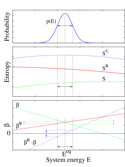
Figure 1: Schematic representation of the dependence on the system energy $E$ of the probability density (above), the entropies $S^{U}$, $S^{R}$ and $S$ (middle), and the inverse temperatures $\beta^{R}$, $\beta$, and the affinity $\Gamma=\beta^{R}-\beta$ (below). The arrows indicate the width of the typical fluctuations of the different variables.

If energy fluctuations are small enough we can expand the function $\Gamma(E)$ about the point $E^{eq}$. A first-order approximation gives:

$$\begin{split}\Gamma=\beta^{R}-\beta\approx\frac{\partial\beta^{R}\left(E^{U}-E\right)}{\partial E}\left(E^{eq}-E\right)-\\ -\frac{\partial\beta\left(E\right)}{\partial E}\left(E-E^{eq}\right)=\phi\Delta E\;,\end{split}$$ (24)

where we have taken into account the fact that $E^{U}$ is fixed and we have defined:

$$\phi\equiv\left.\frac{\partial^{2}S^{U}}{\partial E^{2}}\right|_{E^{eq}}=-\left.\frac{\partial\beta^{R}\left(E\right)}{\partial E}\right|_{E^{eq}}-\left.\frac{\partial\beta\left(E\right)}{\partial E}\right|_{E^{eq}}\;,$$ (25)

which plays the role of an inverse joint heat capacity. Indeed the plots shown in Fig. 1 correspond to such a first-order approximation, where the probability is Gaussian, the entropy densities are parabolas and the inverse temperatures and affinity behave linearly.

Note that within this first-order approximation, condition (22) yields $\langle E\rangle=E^{eq}$. Besides, the fact that $\beta^{R}-\beta\propto\Delta E$ makes (23) an equalty (it is indeed a property of the Schwartz inequality). Thus, replacing (24) into (23), we find

$$\phi\left\langle\left(\Delta E\right)^{2}\right\rangle=1\,.$$ (26)

Hence

$$\left\langle\left(\Delta E\right)^{2}\right\rangle=\left[-\left.\frac{\partial\beta^{R}\left(E\right)}{\partial E}\right|_{E^{eq}}-\left.\frac{\partial\beta\left(E\right)}{\partial E}\right|_{E^{eq}}\right]^{-1}$$ (27)

If we define the system heat capacity $C$ and the reservoir heat capacity $C^{R}$ as

$$-\left.\frac{\partial\beta}{\partial E}\right|_{E^{eq}}=\frac{1}{kT^{2}}\frac{\partial T}{\partial E}=\frac{1}{kT^{2}C}\;,$$ (28)

$$-\left.\frac{\partial\beta^{R}}{\partial E^{R}}\right|_{E^{eq}}=\left.\frac{\partial\beta^{R}}{\partial E}\right|_{E^{eq}}=\frac{1}{kT^{2}}\frac{\partial T}{\partial E}=\frac{1}{kT^{2}C^{R}}\;,$$ (29)

where $T=\left(k\left\langle\beta\right\rangle\right)^{-1}$ stands for the equilibrium temperature, we get:

$$\left\langle\left(\Delta E\right)^{2}\right\rangle=\frac{kT^{2}C^{R}C}{C+C^{R}}\;,$$ (30)

which is essentially the same result obtained by Lindhart, as discussed in Ref. Uffink1999, , but seen from within a different framework. At the same order of approximation we can compute:

$$\langle\Gamma^{2}\rangle=\frac{1}{\left\langle\left(\Delta E\right)^{2}\right\rangle}=\frac{C^{R}+C}{kT^{2}CC^{R}}\;,$$ (31)

$$\langle\left(\Delta\beta^{R}\right)^{2}\rangle=\frac{C}{kT^{2}C^{R}(C^{R}+C)}\;,$$ (32)

$$\langle\left(\Delta\beta\right)^{2}\rangle=\frac{C^{R}}{kT^{2}C(C^{R}+C)}\;,$$ (33)

$$\langle\left(\Delta\beta\Delta\beta^{R}\right)\rangle=\sqrt{\left(\Delta\beta^{R}\right)^{2}\left(\Delta\beta\right)^{2}}=\frac{1}{kT^{2}\left(C^{R}+C\right)}\;.$$ (34)

From the previous equations, for an infinite reservoir ($C^{R}\gg C$) we obtain the expected results

$$\left\langle\left(\Delta E\right)^{2}\right\rangle=kT^{2}C\;,$$ (35)

$$\langle\Gamma^{2}\rangle=\frac{1}{kT^{2}C}\;,$$ (36)

$$\langle\left(\Delta\beta^{R}\right)^{2}\rangle=0\;,$$ (37)

$$\langle\left(\Delta\beta\right)^{2}\rangle=\frac{1}{kT^{2}C}\;,$$ (38)

$$\langle\left(\Delta\beta\Delta\beta^{R}\right)\rangle=0\;.$$ (39)

II.4 Applicability to discrete systems

Even though many macroscopic systems can be studied as continuous, their nature is usually discrete, and, therefore, equations (18) and (19) should be seen as approximations. We will now discuss how to deal with discrete systems.

The main difficulty in the application of equation (19) to discrete systems, is how derivatives should be taken in the definition of intensive variables. We must consider, not only the problem of finding whether defining forward, backward or central derivatives can affect the result, but we must also take into account the fact that $\frac{d}{dx}\ln p$ and $p^{-1}\frac{d}{dx}p$ have different corresponding discrete expressions. Let us discuss two possible definitions.

If we consider the second part of Eq. (2) a possible (centred) definition of $\Gamma$ is

$$\Gamma_{i}\equiv-\frac{\ln p_{i+1}-\ln p_{i-1}}{2}\;,$$ (40)

which is separable if the probability $p$ factorizes. Nevertheless this prescription also raises some problems: since the logarithm goes to minus infinity as probability goes to zero, one must be really careful at the edges of the domain and change the centred prescription to backwards and forward prescriptions.

An alternative definition of $\Gamma_{i}$ is the one suggested from the first part of Eq. (2):

$$\Gamma_{i}\equiv-\frac{p_{i+1}-p_{i-1}}{2p_{i}}\;.$$ (41)

This definition is not separable as a product of terms for the system and the reservoir, not even when the probability factorizes. As a consequence, the concept of intensive variables cannot be thought of as a property of a single system. Instead, in this case, we shall deal with affinities that are a property of each pair of systems in equilibrium. In the first example in the next Section III we will compare the results obtained with the two prescriptions in order to evaluate how much the choice can affect the results for small systems.

III Numerical simulations

In order to discuss the applicability of the above expressions, we will test them in two numerically treatable examples: a non-interacting lattice system (Paramagnetic Ising system) and an interacting lattice system (Ferromagnetic Ising system). We will focus on the validity of expressions (18) and (19) for various universe sizes, various system sizes within each universe and different values for the extensive fixed variables of the universe. Our aim is to deepen our understanding of the validity of these equations.

III.1 Paramagnetic Ising system

Let us firstly analyze the validity of the formalism developed above for a model without interaction. We shall consider a universe consisting of $N^{U}$ non-interacting spins $s_{i}$ that can take two values $\pm 1$, depending on whether they are parallel or antiparallel to an external field $H$ (which is a fixed parameter of the model). The Hamiltonian is given by ${\cal H}=-\sum_{i=1}^{N}s_{i}H$. Since the universe is isolated (constant energy) the number of spins $N^{U}_{+}$ in the $+1$ state and the number of spins $N^{U}_{-}$ in the $-1$ state (fulfilling $N^{U}_{+}+N^{U}_{-}=N^{U}$) are fixed. Therefore, the number of possible configurations of the universe is given by:

$$W=\frac{N^{U}!}{N^{U}_{+}!\left(N^{U}-N^{U}_{+}\right)!}$$ (42)

We now consider a partition of the whole universe into the two sets: the system and the reservoir so that $N^{U}=N^{R}+N$. We will choose the number of spins $N_{+}$ in the $+1$ state in the system as the internal variable of interest in this example (this choice gives simpler expressions than choosing the energy). Its probability function will be given by:

$$\begin{split}p(N_{+})=\frac{N!}{N_{+}!(N-N_{+})!}\\ \times\frac{(N^{U}-N)!}{(N^{U}_{+}-N_{+})!(N^{U}-N-N^{U}_{+}+N_{+})!}\\ \times\frac{N^{U}_{+}!\left(N^{U}-N^{U}_{+}\right)!}{N^{U}!}\;,\end{split}$$ (43)

where $N^{U}$, $N^{U}_{+}$ and $N$ are parameters. Note that the variable $N_{+}$ ranges between the extremes corresponding to its minimum value given by $N_{+}^{min}=\max(0,N^{U}_{+}-N^{U}+N)$ and its maximum value given by $N_{+}^{max}=\min(N^{U}_{+},N)$. Using the probability function (43) we can explicitly compute the average value $\langle N_{+}\rangle$ and its variance as

$$\langle\left(\Delta N_{+}\right)^{2}\rangle=\langle\left(N_{+}\right)^{2}\rangle-\langle N_{+}\rangle^{2}$$ (44)

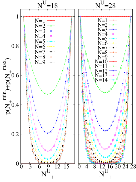
Figure 2: Probability of the boundary states $p(N_{+}^{min})+p(N_{+}^{max})$ as a function of $N^{U}_{+}$ for a paramagnetic system for different universe sizes and system sizes as indicated by the title and legend respectively.

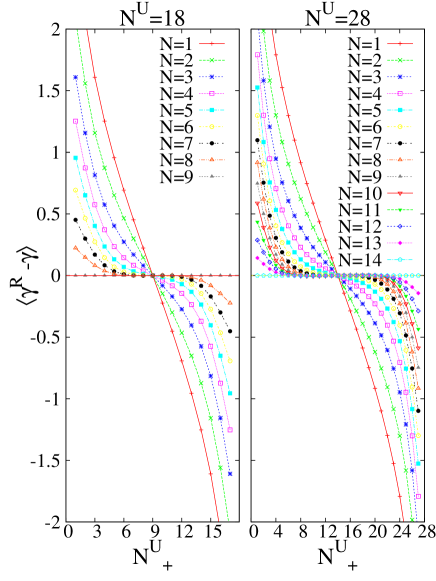
Figure 3: Test of the validity of the equality of the $\langle\gamma\rangle$ and $\langle\gamma^{R}\rangle$ as a function of $N^{U}_{+}$ for a paramagnetic system, using the prescription from Eq. (40)

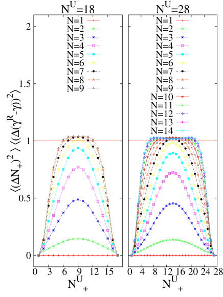
Figure 4: Test of the validity of the uncertainty relation as a function of $N^{U}_{+}$ for a paramagnetic system, using the prescription from Eq. (40). The red line shows the proposed lower bound.

For illustrative purposes, in this first example we compute the probability for the system to reach boundary states $p(N_{+}^{min})+p(N_{+}^{max})$. Fig. 2 shows the value of this probability for two universes of sizes $N^{U}=18$ and $N^{U}=28$ as a function of $N^{U}_{+}$ and for different values of the system size $N$. This result shows that the probability of the boundary states departs from zero when the system or reservoir are too small and when the value of $N_{+}^{U}$ is too close to its extremes and this fact constrains the number of available states in the system.

So far there has been no need to take one of the prescriptions described in section II.4. However, in order to perform the study of the conjugated intensive variables we must now choose one of the prescriptions. The first proposed option, according to Eq. (40), enables us to benefit from the separation of the entropy density. As the spins are non-interacting, when we define the entropy using the logarithm and neglect irrelevant constants, it can be trivially separated as:

$$S(N_{+})=\ln p(N_{+})=S(N_{+})+S^{R}(N^{U}_{+}-N_{+})$$ (45)

with

$$S(N_{+})=\ln\frac{N!}{N_{+}!(N-N_{+})!}$$ (46)

and

$$\begin{split}S^{R}(N^{U}_{+}-N_{+})\\ =\ln\frac{(N^{U}-N)!}{(N^{U}_{+}-N_{+})!(N^{U}-N-N^{U}_{+}+N_{+})!}\end{split}$$ (47)

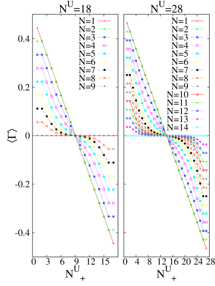
Figure 5: Test of vanishing of the average affinity $\langle\Gamma\rangle$ for a paramagnetic system, using the prescription in Eq. (41)

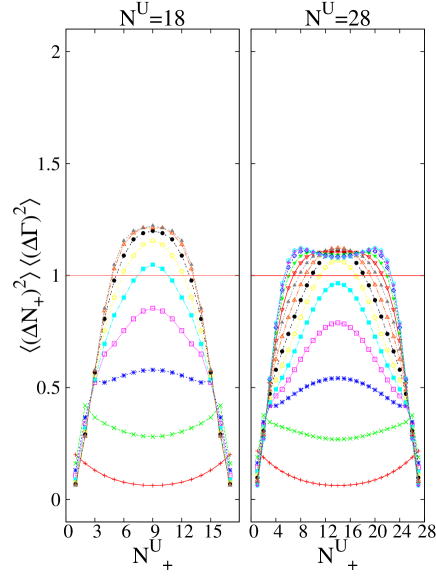
Figure 6: Test of the validity of the uncertainty relation for a paramagnetic system using Eq. (41). The red line shows the proposed lower bound. The symbols correspond to the values of $N$ indicated in the legends of the previous figures.

To estimate the intensive variables of the system ($\gamma$) and reservoir ($\gamma^{R}$) we approximate the derivatives of $S$ and $S^{R}$ by a finite difference scheme. Since the variable $N_{+}$ is bounded, we will use central differences everywhere except at the extremes, where we will use forward or backwards differences. Thus:

$$\begin{split}\gamma=\frac{dS}{dN_{+}}\simeq\frac{S(N_{+}+1)-S(N_{+}-1)}{2}\\ =\ln\sqrt{\frac{(N-N_{+}+1)(N-N_{+})}{(N_{+}+1)N_{+}}}\;,\end{split}$$ (48)

and

$$\begin{split}\gamma^{R}=\frac{dS^{R}}{dN^{R}_{+}}=-\frac{dS^{R}}{dN_{+}}\simeq-\frac{S^{R}(N_{+}+1)-S^{R}(N_{+}-1)}{2}\\ =\ln\sqrt{\frac{(N^{U}-N-N^{U}_{+}+N_{+}+1)(N^{U}-N-N^{U}_{+}+N_{+})}{(N^{U}_{+}-N_{+}+1)(N^{U}_{+}-N_{+})}}\;.\end{split}$$ (49)

Fig. 3 shows the difference $\langle\gamma^{R}-\gamma\rangle$ as a function of $N^{U}_{+}$, for universes of sizes $N=18$ (left panel) and $N=28$ (right panel) and different system sizes $N$ (ranging from $1$ to $N^{U}/2$). Notice that the roles of the system and reservoir are, in this case, symmetric. As can be seen, the difference $\langle\gamma^{R}-\gamma\rangle$ vanishes when $N_{+}^{U}$ (which determines the available energy) is not close to its upper or lower extremes. It is clearly observed that the range of validity of the result in Eq. (20) increases when the system size $N$ approaches half the universe size $N^{U}/2$, since we have more available states and therefore the importance of the boundary states on the computed averages decreases.

Fig. 4 shows the test of the uncertainty relation (21) as a function of the total number of up spins $N^{U}_{+}$. For $N^{U}=18$ and $N^{U}=28$, and different values of $N$. Similar conclusions to those observed in Fig. 3 can be deduced: when $N$ and $N^{U}_{+}$ are far from their boundary values, the uncertainty relation is fulfilled. Only when the fluctuating variable $N_{+}$ is strongly constrained to a tiny number of states by the system size $N$ or the available fixed universe energy $N^{U}_{+}$, do the surface terms neglected in the derivation of the uncertainty relation play a role and the bound is broken.

Alternatively, we can study the second method proposed for discrete systems and define the joint affinity $\Gamma$ as in Eq. (41). In this case, however, it is not possible to separate $\Gamma$ into two terms, one corresponding to the system and another one corresponding to the reservoir. Numerical computation for the same cases studied before allows us to plot the results shown in Figs. 5 and 6. The same qualitative results concerning the validity of (18) and (19) can be concluded. Note that the values of $\langle\Gamma\rangle$ in Fig. 5 are smaller than those in Fig. 3. Therefore, for discrete systems, the choice of the approximation method discussed in section II.4 may affect the results from a quantitative point of view, even in such a simple case.

III.2 Ferromagnetic Ising system

In this second example we study the case of a discrete system with interactions. Since interaction can induce correlations, in this case we should not assume that the entropy density $S^{U}$ is separable and thus we should restrict ourselves to only testing the validity for equations (18) and (19).

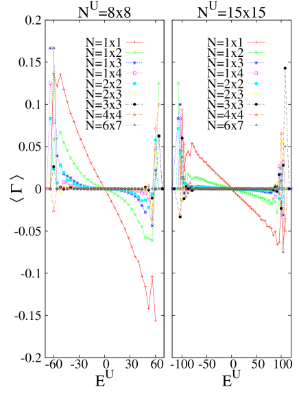
Figure 7: $\left\langle\Gamma\right\rangle$ plotted against the energy of the universe for a 15x15 and a 8x8 universe, and for various sizes of the corresponding systems. As the size of the system increases, the expected value of $\Gamma$ goes to zero, as expected.

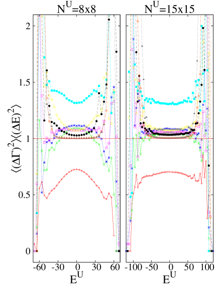
Figure 8: Test for the fluctuation theorem in discrete systems. Symbols are the same as in the previous figure. As in figure 2, the red line shows the proposed lower bound.

Let us consider a universe consisting of an Ising model on a two- dimensional square lattice with size $N^{U}=L^{U}\times L^{U}$, with nearest-neighbour interactions and periodic boundary conditions. The system of interest will be a rectangular subset of spins with size $N=L_{x}\times L_{y}$. Even though a general treatment requires the simultaneous analysis of energy and magnetization fluctuations, in the absence of an external field, it is enough to analyse only the energy. The Hamiltonian of the universe reads

$${\cal H}^{U}=-\sum_{i,j}^{n.n.}s_{i}s_{j}\;,$$ (50)

where $s_{i}=\pm 1$ are the spin variables and the sum extends over all the $2N^{U}$ nearest-neighbour pairs of the universe. Note that the energy of the universe will be discretized in steps $\delta E^{U}=4$ and ranges from $-2N^{U}$ to $2N^{U}$ For any given configuration, the evaluation of the energy of the system will be done by considering that the energy associated with the bonds along the boundary of the system is equally divided between the system and reservoir. Therefore, the energy of the system is discretized in steps $\delta E=1$.

In order to perform a microcanonical analysis of the averages at constant $E^{U}$ we have used the following procedure. We have randomly generated spin configurations and classified them according to the universe energy. Inside the set corresponding to the same value of $E^{U}$ we have computed the fraction of configurations that correspond to every possible value of the energy $E$ of the system and performed a statistical estimation of its probability $p(E)$.

It is important to note that, because of the finite size of the random sample of states that we have generated ($3\times 10^{7}$ configurations), we do not obtain states with an a priori small but non-zero probability. This means that there is a certain number of possible values of $E$ for which we wrongly estimate zero probability. As the logarithmic prescription (40) discussed in II.4 would give problems with infinities at the neighbouring values, we have only used the second prescription given by Eq. (41). Even in this second case, in order to avoid problems with the computation of the variance of $\Gamma$ (for which a $p_{i}$ survives in the denominator), the states with an estimated zero probability have been excluded: it is as if they could not be reached by the system.

Figures 7 and 8 show the results obtained for simulations of a $8\times 8$ and a $15\times 15$ universe, for various sizes of the system. These are qualitatively compatible with those obtained for the system without interactions in Sec. III.1. The uncertainty relations are fulfilled except in the very extreme case in which the number of available states of the system and/or reservoir is so small that the boundary effects are dominant.

IV Discussion and Conclusions

We have shown that uncertainty relations can be established in statistical mechanics when considering a universe (isolated from the outer world) separated into two parts, called the system and reservoir, which are in thermodynamic equilibrium and interact by exchanging ”mechanical properties” such as energy, volume, particles, … If $X_{i}$ is one of these properties corresponding to the system, we have found that the following inequality must be satisfied, $\sqrt{\langle(\Delta X_{i})^{2}\rangle\langle(\Gamma_{i})^{2}\rangle}\geq 1$. Here, $\Gamma_{i}$ is an affinity conjugated to the variable $X_{i}$ which determines the departure from strict equilibrium of actual microscopic configurations of the two interacting systems and which satisfies $\langle\Gamma_{i}\rangle=0$. Furthermore, when the entropy satisfies separability, these affinities simply reduce to the difference $\gamma_{i}^{R}-\gamma_{i}$ of the intensive variable conjugated to $X_{i}$, in the reservoir and the system.

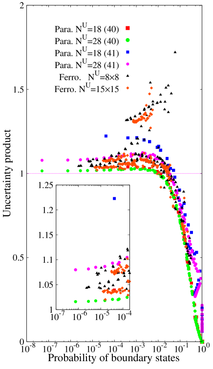
Figure 9: Uncertainty product against the probability of boundary states for the paramagnetic Ising system and the ferromagnetic Ising model. Data includes different universe sizes, system sizes, and different values of the mechanical variables of the universe. We have also included the data corresponding to the two different methods proposed for the evaluation of the affinities for discrete systems, given by Eqs. (40) and (41), indicated in the legend by the numbers between parenthesis. The inset shows a magnification of the region above $1$ for probabilities below $2\times 10^{-4}$.

Assuming that the intensive variable of the reservoir does not fluctuate as expected for very large reservoirs, the proposed inequality reduces to the more standard uncertainty relation involving only system variables

$$\sqrt{\langle(\Delta X_{i})^{2}\rangle\langle(\gamma_{i})^{2}\rangle}\geq 1$$ (51)

Furthermore, assuming that the fluctuations in the system are small, by expanding to first order, the uncertainty relation leads to the following equality:

$$\langle(\Delta X_{i})^{2}\rangle=\frac{1}{\langle(\Delta(\gamma_{i}^{R}-\gamma_{i}))^{2}\rangle}$$ (52)

It is interesting to point out, than within this first-order approximation, when the relevant conjugated variables are the energy and the inverse temperature, combining Eqs. (30) and (33), one gets:

$$\sqrt{\langle(\Delta E)^{2}\rangle\langle(\Delta\beta)^{2}\rangle}=C^{R}/(C+C^{R})\leq 1\;,$$ (53)

where $C$ and $C^{R}$ are the heat capacities of the system and reservoir. Therefore, in this last case fluctuations of inverse temperature are not, in general, expected to be proportional to energy fluctuations Chui1992 . Only in the limit $C/C^{R}\ll 1$ is the standard result $\sqrt{\langle(\Delta E)^{2}\rangle\langle(\Delta\beta)^{2}\rangle}=1$ recovered.

The derivation of the above results has required the assumption that the probability for the boundary states (on the boundary of the set of mechanical variables $\Omega$) vanishes. This assumption, which is reasonable for universes described by continuum variables, might be incorrect for the discrete case, when universes are small or too constrained.

We have numerically studied the validity of the above results in two different mechano-statistical lattice systems: the Ising paramagnet and the Ising ferromagnet. We have found that the uncertainty relations hold except in the case in which the boundary states have a high probability of occurring. In particular, from the examples in section III, we can numerically evaluate a bound for this probability. Fig. 9 shows the uncertainty product $\langle(\Delta X_{i})^{2}\rangle\langle\Gamma_{i}^{2}\rangle$ against the probability of the boundary states for the Ising paramagnet (with the two possible definitions of the affinities for discrete systems given by Eqs.  (40) and (41)) and the Ising ferromagnet. The figure clearly shows that the breakdown of the uncertainity relation may occur only when the probability of the boundary states is above 0.01. In all the other cases, the uncertainty product is larger than one and, in fact, tends to 1 from above when the size of the universe increases, as can be seen in the inset of Fig.9.

These results are relevant from an experimental point of view. Focusing on the case of the energy $E$ and the inverse of temperature $\beta$ as conjugated variables, we can identify the reservoir with a given body and the system with the thermometer used to measure its temperature. Commonly, the thermometer is chosen so that it has a heat capacity much smaller than the heat capacity of the body. However, for small bodies, when the heat capacity of the thermometer and the body are comparable, the results derived here must be taken into account: (i) the inverse temperature $\langle\beta\rangle$ measured by the thermometer con strongly fluctuate, but still its average value must be identified with the average of the inverse temperature of the body $\langle\beta^{R}\rangle$; and (ii) the fluctuations of the difference $\beta^{R}-\beta$ should be related to the energy fluctuations through the proposed uncertainty relation.

Future extensions of this work will deal with the analysis of systems described by continuous variables, where direct counting of states is not straightforward. The results will be presented elsewhere.

- (1) D. Ter Haar, Rev. Mod. Phys. 27, 289 (1955).
- (2) K. Huang, Statistical Mechanics, Wiley. (1987)
- (3) C.Kittel, Phys. Today 41, 93 (1988).
- (4) T.C.P.Chui, D.R.Swanson, M.J.Adriaans, J.A.Nissen, and J.A.Lipa, Phys. Rev. Lett. 69, 3005 (1992).
- (5) It seems that Bohr was reluctant to admit an Uncertainty Principle for thermodynamic systems see N. Bohr, Collected Works, Vol. 6 pp. 316-330. 376-377.
- (6) J. Uffink and J. van Lith, Found. Phys., 29, 655 (1999), and references therein.
- (7) L. Velázquez and S. Curilef, Uncertainty Relations of Statistical Mechanics, Mod. Phys. Lett. A, 23, 3551-3562 (2009).
- (8) B. Mandelbrot, Ann. Math Stat., 33, 1021 (1962).
- (9) R. Gilmore, Phys. Rev. A, 31, 3237 (1985).
- (10) C.Kittel and B.Mandelbrot, Phys. Today 42, 154 (1989).
- (11) M.Falcini, D.Villamaina, A.Vulpiani, A.Puglisi and A.Sarracino, Am. J. Phys. 79. 777 (2011).
- (12) O.Redlich, Journ. Chem. Education 47, 740 (1970).
- (13) A. Einstein, Phys.Z. 10: 185 (1909); English translation in: The Collected Papers of Albert Einstein, Vol. 2 (Princeton University Press, New Jersey, 1993).
- (14) A. Einstein, Ann. Physik 33: 1275-1298 (1910); English translation in: The Collected Papers of Albert Einstein, Vol. 3 (Princeton University Press, New Jersey, 1993).