Dark Matter and Dark Energy via Non-Perturbative (Flavour) Vacua

Abstract

A non-perturbative field theoretical approach to flavour physics (Blasone-Vitiello formalism) has been shown to imply a highly non-trivial vacuum state. Although still far from representing a satisfactory framework for a coherent and complete characterization of flavour states, in recent years the formalism has received attention for its possible implications at cosmological scales. In a previous work, we implemented the approach on a simple supersymmetric model (free Wess-Zumino), with flavour mixing, which was regarded as a model for free neutrinos and sneutrinos. The resulting effective vacuum (called flavour vacuum) was found to be characterized by a strong SUSY breaking. In this paper we explore the phenomenology of the model and we argue that the flavour vacuum is a consistent source for both Dark Energy (thanks to the bosonic sector of the model) and Dark Matter (via the fermionic one). Quite remarkably, besides the parameters connected with neutrino physics, in this model no other parameters have been introduced, possibly leading to a predictive theory of Dark Energy/Matter. Despite its oversimplification, such a toy model already seems capable to shed some light on the observed energy hierarchy between neutrino physics, Dark Energy and Dark Matter. Furthermore, we move a step forth in the construction of a more realistic theory, by presenting a novel approach for calculating relevant quantities and hence extending some results to interactive theories, in a completely non-perturbative way.

Introduction

Neutrino Flavour Oscillation is nowadays a fairly well-established fact, thanks to a wide range of experimental evidences Strumia:2006db. A simple quantum mechanical model (based on the work of Pontecorvo, Maki, Nagawa, and Sakata Pontecorvo:1957qd; Pontecorvo:1967fh; Gribov:1968kq; Maki:1962mu) is commonly considered as sufficient for accounting for experimental data. However, this hides non-trivial difficulties in the formulation of flavour oscillations in a Quantum Field Theoretical (QFT) framework Beuthe:2001rc. Flavour states indeed do not represent correct asymptotic states (by definition, since their oscillating behaviour), which are required in the usual perturbative approach to QFT (in the Lehmann, Symanzik and Zimmermann scheme).
More than a decade ago, a non-perturbative approach for building flavour states was suggested by Blasone, Vitiello and coworkers (BV formalism for flavour physics) Blasone:1995zc. A first version was proposed in 1995 Blasone:1995zc, but some inconsistencies in the derivation of oscillation formulae were noticed Fujii:1998xa; Blasone:1999jb; Fujii:2001zv; Blasone:2001sr shortly after; a revisited version, in which these discrepancies were clarified and removed, was suggested and developed Blasone:1998hf; Blasone:2001du; Ji:2001yd; Ji:2002tx; Blasone:2002jv later on Beuthe:2001rc. However, for some aspects, the formalism remains controversial and its physical relevance is still matter of debate Giunti:2003dg; Giunti:2006fr; Blasone:2005ae.
The approach correctly reduces to the common quantum mechanical approach in the small (neutrinos) mass limit, but leads to corrections to those formulas that are currently beyond experimental sensitivity Beuthe:2001rc; Capolupo:2004av. However, perhaps the most interesting feature of BV formalism is the non-trivial vacuum (called flavour vacuum) implied by the theory. Such a flavour vacuum (which can be regarded as a vacuum condensate) represents the physical state with no (flavour) particles in it. Despite being merely an “empty” state, the flavour vacuum is characterized by a rich structure revealed by the non-vanishing expectation value of the stress-energy tensor and the related equation of state. Within BV formalism one is able to fully describe it at a non-perturbative level, and its features depend on the specific model considered (spin, interactions, number of particles characterized by flavour mixing, etc.).
In a series of papers it was suggested that the flavour vacuum might behave as a source of Dark Energy Blasone:2004hr; Blasone:2004yh; Capolupo:2006et; Capolupo:2006re; Capolupo:2008rz; Capolupo:2007hy; Blasone:2007iq; Blasone:2008rx; Blasone:2007jm; Blasone:2006ch. Recently, it has been shown that in a simple supersymmetric (Wess-Zumino) model with flavour mixing, in which two Majorana fields, two scalars and two pseudo-scalars were present (a simple model for neutrinos and sneutrinos), the flavour vacuum was actually characterized by a strong Supersymmetry breaking Mavromatos:2010ni; Capolupo:2010ek. In the present work we argue that this breaking is the origin of an interesting phenomenology, that might shed some lights both on the Dark Energy and the Dark Matter problem. More precisely, in the supersymmetric context of Mavromatos:2010ni; Capolupo:2010ek, the flavour vacuum can be thought as made of two different fluids that fill in all universe: a first one related to the bosonic sector of the model, and a second induced by the fermionic one. The former is characterized by negative pressure, equal in modulus to its energy density (acting as a source of Dark Energy). The latter is characterized by zero pressure, giving rise to a source of Cold Dark Matter.

The first part of the paper (Section I) will be dedicated to review BV formalism, complementing the original literature with a discussion on non-perturbative theories and Fock spaces.

In the second part of the paper (Section II) we shall explore in details the phenomenology of the model studied in Mavromatos:2010ni; Capolupo:2010ek. We shall clarify why the flavour vacuum is a good Dark Energy and Dark Matter candidate, with emphasis on this latter. More importantly, we will explain how to relate all parameters of the model to observational data. This is a quite important aspect of the approach: the model introduces very few parameters which are all related to neutrino physics. Hopefully, more realistic models will not rely on uncontrolled free parameters, leading to a truly falsifiable theory for both Dark Energy and Dark Matter. A first encouraging result in this direction comes already from the simple model here studied: this is indeed fairly consistent with a choice of the parameters modeled on real world data, as we shall see in the relevant section.

A first step towards more realistic models will be moved in the last part of this work (Section III). We will present a novel method for calculating relevant quantities, specifically thought for analyzing the features of the flavour vacuum, which might enable us to study interactive theories completely at a non-perturbative level. In particular, we shall show how, under reasonable assumptions, the method can discriminate which interactions preserve the behaviour of the condensate as Dark Energy/Matter source.

I BV Formalism

Neutrino oscillations can be described in a non-relativistic quantum mechanical framework by constructing particle states, labelled by a flavour number, that are not eigenstates of the Hamiltonian. In its simplest formulation for two distinct flavours, the Pontecorvo model, flavour states are constructed as follow Bilenky:2010zza: rCl — ν_A ⟩&=cosθ— ν_1 ⟩ +sinθ— ν_2 ⟩
— ν_B ⟩=-sinθ— ν_1 ⟩ +cosθ— ν_2 ⟩ where $|\nu_{1}\rangle$ and $|\nu_{2}\rangle$ are massive eigenstate of the free Hamiltonian (particles with well defined mass $m_{i}$, with $i=1,2$), and from which rCl ℘_A→B&=—⟨ν_B— ν_A(t) ⟩—^2=—⟨ν_B —e^-iH t— ν_A ⟩—^2
=sin^2 θsin^2(ω1(k) t-ω2(k) t2) with $\omega_{i}(k)\equiv\sqrt{\vec{k}^{2}+m_{i}^{2}}$, describing the non-vanishing probability of a flavoured particle with momentum $\vec{k}$ to be created with a certain flavour ($A$) and be detected later on with a different flavour ($B$).

The form of the transformation between flavoured and massive particles (I) is reflected in the relativistic field formalism by the relation rCl ν_A(x)&= ν_1 (x) cosθ+ν_2 (x) sinθ
ν_B(x)= -ν_1 (x) sinθ+ν_2 (x) cosθthat connects flavour fields $\nu_{A}$, $\nu_{B}$ with massive ones $\nu_{1}$, $\nu_{2}$. Such a relation is connected with the linearization of the following Lagrangian for free spin-$\nicefrac{{1}}{{2}}$ fields

$$\mathcal{L}=i\bar{\nu}_{A}(x)\partial\!\!\!/\nu_{A}(x)+i\bar{\nu}_{B}(x)\partial\!\!\!/\nu_{B}(x)+\\ -m_{A}\bar{\nu}_{A}(x)\nu_{A}(x)-m_{B}\bar{\nu}_{B}(x)\nu_{B}(x)+\\ -m_{AB}\left(\bar{\nu}_{A}(x)\nu_{B}(x)+\bar{\nu}_{B}(x)\nu_{A}(x)\right)$$ (1)

which becomes

$$\mathcal{L}=i\bar{\nu}_{1}(x)\partial\!\!\!/\nu_{1}(x)+i\bar{\nu}_{2}(x)\partial\!\!\!/\nu_{2}(x)+\\ -m_{1}\bar{\nu}_{1}(x)\nu_{1}(x)-m_{2}\bar{\nu}_{2}(x)\nu_{2}(x)$$ (2)

when rClm_A&=m_1cos^2 θ+m_2 sin^2 θ
m_B=m_1 sin^2 θ+m_2 cos^2 θ
m_AB= (m_2-m_1) sinθcosθ.

However, in the field-theoretical framework the decomposition of the fields (I) into ladder operators associated with flavour particle states is highly non-trivial Beuthe:2001rc. It has been shown, indeed, that states defined as the relativistic equivalent of (I), for which $|\nu_{1,2}\rangle$ belongs to the mass-$m_{1,2}$ irreducible representation of the Poincaré group, are not eigenstates of the flavour charge operators Blasone:2006jx; Blasone:2008ii, which for the theory (1) read Blasone:2008ii rCl Q_A(t)&=∫d→x  ν^†_A(x)ν_A(x),
Q_B(t)=∫d→x  ν^†_B(x)ν_B(x).

BV formalism compensate for this Blasone:1995zc; Hannabuss:2000hy; Ji:2002tx, by defining appropriate flavour eigenstates via the action of a certain operator $G_{\theta}$ on massive states:

$$|\vec{k}_{1},f_{1};\vec{k}_{2},f_{2};\vec{k}_{3},f_{3};...\rangle\equiv\\ G^{\dagger}_{\theta}|\vec{k}_{1},m_{(1)};\vec{k}_{2},m_{(2)};\vec{k}_{3},m_{(3)};...\rangle$$ (3)

where $|\vec{k}_{1},f_{1};\vec{k}_{2},f_{2};\vec{k}_{3},f_{3};...\rangle$ denotes a state with different flavour particles described by their momenta $\vec{k}_{i}$ and their flavours $f_{i}=A,B$, whereas $|\vec{k}_{1},m_{(1)};\vec{k}_{2},m_{(2)};\vec{k}_{3},m_{(3)};...\rangle$ denotes a state with different massive particles described by their momenta $\vec{k}_{i}$ and their masses $m_{(i)}=m_{1},m_{2}$, defined from the linearized theory (2). The operator $G_{\theta}$ is defined by the equations: rCl ν_A(x)&= G^-1_θ ν_1 (x) G_θ
ν_B(x)= G^-1_θ ν_2 (x) G_θ and its explicit form depends on the specific theory considered. For the theory (1), $G_{\theta}$ is written as Blasone:1995zc

$$G_{\theta}(t)=e^{\frac{\theta}{2}\int d\vec{x}\left(\nu^{\dagger}_{1}(x)\nu_{1}(x)-\nu^{\dagger}_{1}(x)\nu_{2}(x)\right)}.$$ (4)

Among all flavour states defined in the BV approach, the one called flavour vacuum and defined by

$$|0\rangle_{f}\equiv G^{\dagger}_{\theta}|0\rangle$$ (5)

plays a special role, since it represents the physical vacuum. In this context, by physical vacuum we mean the state that represents the physical empty state, i.e. with no particle in it. Since only particles with well defined flavour, rather than mass (i.e. Hamiltonian eigenstates), can be created/detected, one expects the physical vacuum to be represented by the state that counts no flavour particles in it. It can be shown that this is state is $|0\rangle_{f}$, rather than $|0\rangle$ Blasone:1995zc.

Furthermore, it has been proven that all flavour states $|\vec{k}_{1},f_{1};\vec{k}_{2},f_{2};\vec{k}_{3},f_{3};...\rangle$ are orthogonal to each massive state $|\vec{k}_{1},m_{(1)};\vec{k}_{2},m_{(2)};\vec{k}_{3},m_{(3)};...\rangle$, and therefore $\langle 0|0\rangle_{f}=0$ follows as a particular case. This result enables us to talk of a Fock space for flavour states, in opposition of the usual Fock space, whose basis is given by $\{|\vec{k}_{1},m_{(1)};\vec{k}_{2},m_{(2)};\vec{k}_{3},m_{(3)};...\vec{k}_{n},m_{(n)}\rangle\mid\forall n\in\mathbb{N}\}$.

The orthogonality of the two spaces is not very surprising if one regards BV formalism as a non-perturbative approach to the interactive theory defined by (1).

In the Second-quantization framework, the Hilbert space representing physical states is defined by vectors in the number occupation representation: assuming that a single-particle state can be classified by a discrete set of states labeled by the index $i=1,2,3,...$, a vector representing a many-particle state can be identified by the number $n_{i}$ of particles occupying the $i$-th state and it is denoted with $|n_{1},n_{2},n_{3},...\rangle$; the Hilbert space of physical states $\mathfrak{H}$ is therefore defined as the vector space generated by the basis $\{|n_{1},n_{2},n_{3},...\rangle\}$. For bosons $n_{i}\in\mathbb{N}_{0}$, whereas for fermions $n_{i}=0,1$. It can be shown that in both cases the set $\{|n_{1},n_{2},n_{3},...\rangle\}$ is uncountable and therefore $\mathfrak{H}$ is non-separable Umezawa:1982nv. In particle physics a separable subset of $\mathfrak{H}$, a Fock space that we will denote with $\mathfrak{F_{0}}$, is usually considered Streater:1989vi. $\mathfrak{F_{0}}$ carries an irreducible representation of the Poincaré group and particle states belonging to it have well-defined mass and spin. Such a subset is spanned by the countable basis of all states with an arbitrary, yet finite in total, number of free particles. Although this basis does not fully describe $\mathfrak{H}$ (for instance the vector $|1,1,1,...\rangle$ which counts an infinite number of particles is not included), it is sufficient for accounting for scattering processes at a perturbative level. In the usual perturbation theory all interactive processes are indeed approximated by means of a superposition of a finite number of free particle states. This is quite clear in the functional formalism, when Feynman diagrams are considered. In a simplified picture of this framework, a scattering process is represented by a graph with a certain number of external legs (incoming and outgoing particles). The total number of internal lines is connected to the precision of the approximation used in the perturbative expansion: the higher the order of the perturbation, the higher the number of vertices, and therefore the higher the number of internal lines involved. Each line can be naïvely interpreted as a single free particle state, which is emitted in the starting vertex and then absorbed in the ending one. At each order in perturbation theory, a finite number of free particle states enters in the description of the scattering process. However, under the assumption that the perturbative series converges, its limit would be described by an infinite number of lines/one-free-particle-states. In bra-ket formalism such a limit state would therefore be represented by a vector of $\mathfrak{H}$, the space of all physical states, but not of $\mathfrak{F_{0}}$, the space of states with finite number of free particles. With this example we want to remark the non-trivial difference existing from a free theory and an interactive one: we can express interactive processes in terms of free states (which have no direct physical meaning or interpretation, being just a basis in which we choose to express our process) but only in a weakly-interactive/perturbed framework. A full non-perturbative treatment for interactive particle states requires subspaces of $\mathfrak{H}$, that are orthogonal to the Fock space of free states $\mathfrak{F_{0}}$ Haag:1955ev.

Coming back to our case, a Lagrangian with flavour mixing, such as (1), can be regarded as an interactive theory, thanks to its non-diagonal terms. Flavour particle states defined à la BV form a Fock space $\mathfrak{F_{f}}$ that is therefore orthogonal to $\mathfrak{F_{0}}$. In other words, we could express flavour states in a perturbative way by means of $\mathfrak{F_{0}}$; however, BV formalism enables us to construct flavour states in a completely non-perturbative manner, and therefore it requires states that are part of $\mathfrak{H}$ but not of $\mathfrak{F_{0}}$.

Different Fock spaces are ordinarily used in QFT on curved backgrounds and other contexts Birrell:1982ix; calzetta2008nonequilibrium. In the former, for instance, one identifies Fock spaces for physical states in flat regions. However, these Fock spaces do not coincide (they are different/orthogonal subset of $\mathfrak{H}$) if the regions are not connected and curved regions exist in between. As a consequence, the vacuum defined by an observer in a certain region is not necessarily described by the state with no particles by an observer in another region. The particle creation phenomenon may occur: a state that is empty for an observer can actually contain particles according with a different observer. This mechanism characterizes both of the two main results of QFT in curved spacetime: the Unruh effect Unruh:1976db and the Hawking radiation Hawking:1974sw.

In a formal analogy, BV formalism introduces a ground state, called flavour vacuum, which is not as trivial as the ground state for the free theory. As already said, since it is the state in which no flavour particles are present, it correctly represents the physical vacuum. Even though it is empty, it is characterized by a non-zero expectation value of the stress-energy tensor ${}_{f}\langle 0|T_{\mu\nu}|0\rangle_{f}$, whose effects must be gravitationally testable. This is true as long as we fix as zero-point of our theory the usual vacuum $|0\rangle$ for the free theory and belonging to $\mathfrak{F_{0}}$, or, in other words, we consider the usual normal ordering ${}_{f}\langle 0|:T_{\mu\nu}:|0\rangle_{f}\equiv_{f}\langle 0|T_{\mu\nu}|0\rangle_{f}-\langle 0|T_{\mu\nu}|0\rangle$, which is valid in perturbation theory as well as in this non-perturbative approach. One commonly refers to the flavour vacuum as a condensate for the following reason: once expressed in terms of particles with well defined mass (eigenstates of the Hamiltonian), the flavour vacuum contains an non-vanishing number of those particles, per unit of volume. In our example, they are characterized by the following distribution over the momentum space Capolupo:2004av

$$_{f}\langle 0|n(\vec{k})|0\rangle_{f}=\frac{\sin^{2}\theta}{4\pi^{3}}\frac{\omega_{1}(k)\omega_{2}(k)-m_{1}m_{2}-k^{2}}{\omega_{1}(k)\omega_{2}(k)}$$ (6)

with $n(\vec{k})\equiv\sum_{r}(a_{1}^{r\dagger}(\vec{k})a_{1}^{r}(\vec{k})+a_{2}^{r\dagger}(\vec{k})a_{2}^{r}(\vec{k}))$, $k\equiv|\vec{k}|$, and $a_{i}^{r(\dagger)}$ representing ladder operators for particles with well-defined mass. However, since the physical degrees of freedom of the theory are flavour particles (the only kind of particle that can be produced and detected), the interpretation as a gas or collection of particles remains at a mere mathematical level, the flavour vacuum being absolutely “empty” from a physical point of view (in the sense that no flavoured particles are present in it), and only characterized by a non vanishing stress-energy tensor expectation value which is detectable via gravitational effects.

The features of the flavour vacuum depend on the model considered and a preliminary investigation on a simple supersymmetric model Mavromatos:2010ni showed that it might behave very differently, according with the spin of the particles involved.

II Phenomenology of a SUSY Flavour Vacuum

II.1 Free WZ à la BV

Our interest in BV formalism was firstly motivated by physics beyond the Standard Model. The Wess-Zumino model here discussed has been considered in Mavromatos:2010ni after two works in which the flavour vacuum has been regarded as an effective vacuum arising in a string-theoretical framework mavrosarkar; Mavromatos:2009rf. Indeed, a specific model from the braneworld scenario, called D-particle foam model Mavromatos:2006yy; Mavromatos:2005bu; Mavromatos:2008bz; Ellis:2004ay; Ellis:2005ib, seems to explain neutrino flavour oscillations in terms of flavour oscillation of fundamental strings, in presence of a “cloud” (or foam) of point-like topological defects in the bulk space. In the spirit of weak coupling string theory, the interaction between the foam and strings/branes in the theory can be regarded as “vacuum defects” from the point of view of a macroscopical observer. Therefore it has been suggested that BV formalism, together with its “flavour vacuum” condensate, might provide a suitable description of the low energy limit of the model.

In Mavromatos:2010ni we presented the behaviour of the flavour vacuum, in a simple supersymmetric theory. The model that was considered involves two free real scalars $S_{A}(x)$, $S_{B}(x)$ with mixing, two free real pseudo-scalars $P_{A}(x)$, $P_{B}(x)$ with mixing and two free Majorana spinors $\psi_{A}(x)$, $\psi_{B}(x)$ with mixing:

$$\mathcal{L}=\!\!\!\sum_{\iota=A,B}\Big{[}\partial_{\mu}S_{\iota}(x)\partial^{\mu}S_{\iota}(x)+\partial_{\mu}P_{\iota}(x)\partial^{\mu}P_{\iota}(x)+\\ +i\bar{\psi}(x)\partial\!\!\!/\psi_{\iota}(x)\Big{]}-\!\!\!\sum_{\iota,\kappa=A,B}\Big{[}m_{\iota\kappa}^{2}S^{2}_{\iota}(x)+m_{\iota\kappa}^{2}S^{2}_{\iota}(x)+\\ +m_{\iota\kappa}\bar{\psi}(x)_{\iota}\psi_{\kappa}(x)\Big{]}$$ (7)

with $m_{AB}=m_{BA}$. Terms involving products of fields of different flavours disappear when one expresses the model in terms of new fields, obtained by appropriate rotations of the previous ones: rClϕ_A(x)&=cosθϕ_1(x)+sinθϕ_2(x)
ϕ_B(x)=-sinθϕ_1(x)+cosθϕ_2(x) with $\phi=S,P,\psi$, leading to

$$\mathcal{L}=\sum_{i=1,2}\Big{[}\partial_{\mu}S_{i}(x)\partial^{\mu}S_{i}(x)-m_{i}^{2}S_{i}^{2}(x)+\\ +\partial_{\mu}P_{i}(x)\partial^{\mu}P_{i}(x)-m_{i}^{2}P_{i}^{2}(x)+\\ +\bar{\psi}_{i}(x)(i\partial\!\!\!/-m_{i})\psi_{i}(x)\Big{]}.$$ (8)

From this latter it is possible to build the usual Fock space for massive particles, previously denoted as $\mathfrak{F_{0}}$, which has as ground state the “massive” vacuum $|0\rangle$. The flavour vacuum is hence defined as

$$|0\rangle_{f}\equiv e^{\theta\int d\vec{x}\left(X_{12}(x)-X_{21}(x)\right)}|0\rangle$$ (9)

with

$$X_{12}(x)\equiv\frac{1}{2}\psi^{\dagger}_{1}(x)\psi_{2}(x)+i\dot{S}_{2}(x)S_{1}(x)+i\dot{P}_{2}(x)P_{1}(x).$$ (10)

Its features have been explored via its stress-energy tensor expectation value, being

$$T_{\mu\nu}(x)=\!\!\!\sum_{i=1,2}\!\Big{[}2\partial_{\left(\mu\right.}S_{i}(x)\partial_{\left.\nu\right)}S_{i}(x)+2\partial_{\left(\mu\right.}P_{i}(x)\partial_{\left.\nu\right)}P_{i}(x)+\\ +i\bar{\psi}_{i}(x)\gamma_{\left(\mu\right.}\partial_{\left.\nu\right)}\psi_{i}(x)\Big{]}-\eta_{\mu\nu}\mathcal{L}.$$ (11)

It has been shown that the flavour vacuum behaves as a perfect relativistic fluid, i.e.

$${}_{f}\langle 0|T_{\mu\nu}|0\rangle_{f}=diag\{\rho,\mathsf{P},\mathsf{P},\mathsf{P}\}$$ (12)

with

$$\begin{split}\rho\equiv&{}_{f}\langle 0|T_{00}(x)|0\rangle_{f}=\\ =&\sin^{2}\theta\frac{(m_{1}-m_{2})^{2}}{2\pi^{2}}\int_{0}^{K}\!\!\!\!dk\;k^{2}\left(\frac{1}{\omega_{1}(k)}+\frac{1}{\omega_{2}(k)}\right)\end{split}$$ (13)

$$\begin{split}\mathsf{P}\equiv&{}_{f}\langle 0|T_{jj}(x)|0\rangle_{f}=\\ =&-\sin^{2}\theta\frac{m_{1}^{2}-m_{2}^{2}}{2\pi^{2}}\int_{0}^{K}\!\!\!\!dk\;k^{2}\left(\frac{1}{\omega_{2}(k)}-\frac{1}{\omega_{1}(k)}\right)\end{split}$$ (14)

$\rho$ representing its energy density, $\mathsf{P}$ its pressure and $K$ a momentum cutoff (cf Mavromatos:2010ni; Capolupo:2010ek).

In particular, disentangling the contribution of the bosonic sector from the fermionic one, one finds

$$\rho_{b}=\sin^{2}\theta\int_{0}^{K}\!\!dk\frac{k^{2}}{\pi^{2}}\left(\omega_{1}(k)+\omega_{2}(k)\right)\times\\ \times\left(\frac{\left(\omega_{1}(k)-\omega_{2}(k)\right)^{2}}{2\omega_{1}(k)\omega_{2}(k)}\right)$$ (15)

$$\rho_{f}=\sin^{2}\theta\int_{0}^{K}\!\!dk\frac{k^{2}}{\pi^{2}}\left(\omega_{1}(k)+\omega_{2}(k)\right)\times\\ \times\left(\frac{\omega_{1}(k)\omega_{2}(k)-m_{1}m_{2}-k^{2}}{\omega_{1}(k)\omega_{2}(k)}\right)$$ (16)

$$\mathsf{P}_{b}=-\rho_{b},\;\;\;\;\;\;\mathsf{P}_{f}=0$$ (17)

in which the standard normal order has being adopted.

II.2 Flavour vacuum as a source of Dark Matter

An important result emerges from the above outlined analysis: the equation of states $w\equiv\mathsf{P}/\rho$ for the bosonic and the fermionic sectors are different, $w_{b}=-1$ and $w_{f}=0$ holding. The emphasis on the novelty of this SUSY breaking mechanism has already being remarked Mavromatos:2010ni. We are now aimed to explore the interesting phenomenology connected with such a result. Our simple model implies a physical vacuum that is a combination of two fluids which behave quite differently: both permeate the empty space uniformly and statically, but one has a cosmological-constant-like behaviour ($w=-1$), while the other behaves as dust ($w=0$). The role of the flavour vacuum as source of Dark Energy (which now is played only by the bosonic sector of the theory) has been extensively discussed in literature Blasone:2004hr; Blasone:2004yh; Capolupo:2006et; Capolupo:2006re; Capolupo:2008rz; Capolupo:2007hy; Blasone:2007iq; Blasone:2008rx; Blasone:2007jm; Blasone:2006ch. Here we present a new feature of the flavour vacuum: its contribution to Dark Matter.

Dark Matter is the name given to unknown sources of gravitational effects, whose presence, primarily within and around galaxies, has been established by many astrophysical data Bertone:2004pz; Jungman:1995df. Numerical simulations of structure formation have shown that “hot” (relativistic) particles cannot explain the observed structures at galactic scales, therefore Dark Matter is expected to be made out of fairly massive and “cold” (non-relativistic) particles. Big-Bang nucleosynthesis limits on the average baryonic content of the Universe exclude that (the majority of) Dark Matter is made out of ordinary baryonic matter (i.e. atoms). Furthermore, although “dark”, in the sense that does not emit nor absorb light (i.e. electromagnetically neutral), Dark Matter might couple to ordinary matter in other ways (besides gravity); however, arguments on its density and thermal production at early times imply that such a coupling must be weak.

Both astrophysics and particle physics have been proposing suitable candidates for Dark Matter through the last three decades, giving rise to an enormous wealth of choice. However, because of the absence of direct detections and the lack of predictions by theoretical models, plagued by an undesirable abundance of free parameters, the nature of Dark Matter remains elusive.

The fermionic sector of the flavour vacuum in the model here presented clearly fulfills basic requests for a Dark Matter candidate: it contributes to the energy content of the universe; it is “dark” (i.e. it is an electromagnetically neutral object, since (s)neutrino fields do not couple with the electromagnetic field); furthermore, it does not interact with any other of the SM particles (excluding gravitational effects), being the empty state for the (s)neutrino sector; unlike its bosonic counterpart, it is purely pressureless.

A possible concern about its uniform distribution in space, in contrast with the observed distribution of Dark Matter which is usually gathered in clusters around and inside galaxies, can be easily dispelled by recalling that we are actually modeling a simple “empty” universe. If a non-uniform matter distribution is considered in our toy universe in addition to the flavour vacuum, it would start to interact gravitationally with our vacuum condensate. Thanks to initial irregularities in the matter distribution, we expect them to form clusters via gravitational instability (gravity tends to enhance irregularities, pulling matter towards denser regions Liddle:2009zz), as the system evolves with time. It is known that such an effect, on the other hand, does not necessarily occurs for Dark Energy-like fluids amendola, as the bosonic component of the flavour vacuum, which can persist in their state of spatial uniformity even in presence of clustered matter. The evolution of our flavour vacuum, considering both its bosonic and fermionic components, in presence of other matter and gravitational interaction, represents necessarily an object of future studies.

II.3 Testability

An interesting aspect of the model concerns the interplay between the two fluids. Supersymmetry imposes that the energy density of the bosonic component is tied up to the energy density of the fermionic component; in a more realistic theory, therefore, one should be able to reproduce the current experimental value of the ratio between the Dark Energy density and the Dark Matter energy density ($\sim 2.8$), in the optimist belief that the flavour vacuum is the only responsible for both of them. The role of a curved background in the formulation of the theory might be crucial, since the energy density of a dust-like fluid gets diluted by the expansion of the universe, whereas such an effect does not occur for a cosmological-constant type, and therefore the ratio between those two quantities changes dramatically with time.

Within a momentum cutoff regularization framework, as the one here presented, the two energy densities depend on such a cutoff, which is the same for both quantities. The ratio between them can in general be cutoff dependent, as it actually is in the case here presented. On one side, one might hope that in a more realistic theory (on a curved background, for instance) the ratio might be cutoff independent. On the other hand, one could consider the opposite situation, in which the ratio varies with the cutoff, as highly desirable: if the ratio is fixed from the cutoff, the same value for the cutoff would also fix the value of the energy. This implies that once the cutoff is decided on the basis of experimental data on the ratio, the model gives a precise prediction for the absolute values of the energy densities, which can be compared with their observational estimates.

In order to illustrate these ideas we will present a concrete example. Let us assume that our supersymmetric model is effective up to the energy scale $K$ (which comes from deeper theories, as, for instance, in Mavromatos:2010ni ). In the standard Big-Bang picture, this means that when the universe cools down to that energy, the flavour vacuum starts to be the effective description of the vacuum state of the (unknown) underlying theory. We call $t_{0}$ the time corresponding with this transition and $a_{0}$ the corresponding scale factor.

In our toy universe, we assume that at $t_{0}$, in absence of any other sources of energy or matter, the energy/matter content of our toy universe is only due to the flavour vacuum. Moreover, we assume that it can be describe, at a classic level (i.e. on sufficiently large scales), in terms of two fluids: a first one, due to the bosonic component of the flavour vacuum and described by $\rho_{b}$ and $w=-1$, and a second one, due to its fermionic component and described by $\rho_{f}$ and $w=0$. We will regard the bosonic component as the only source of Dark Energy and the fermionic as the only source of Dark Matter. Both $\rho_{b}$ and $\rho_{f}$ are function of the following parameters: (s)neutrino masses, mixing angles, and the cutoff $K$. If we know (from observations) the neutrino masses and mixing angles, and we can constrain parameters induced by SUSY breaking, the cutoff is the only parameter left to determine.

As our toy universe expands, we assume that the two fluids obey Einstein equations and therefore they scale as

$$\begin{split}\rho_{f}(t)\;\;a(t)^{3}=&\rho_{f}\;\;a_{0}^{3}\\ \rho_{b}(t)=&\rho_{b}.\\ \end{split}$$ (18)

This means that today their value is

$$\begin{split}\rho_{f}(t_{now})=&\rho_{f}\;\;a_{0}^{3}\\ \rho_{b}(t_{now})=&\rho_{b}.\\ \end{split}$$ (19)

respectively, being $a(t_{now})=1$ by convention. Those two quantities depends on the following parameters: (s)neutrino masses, mixing angles, cutoff energy, scale factor at $t_{0}$. Provided with these expressions, we can then test our model in two ways.

1. If observational data enable us to constrain (s)neutrino masses, mixing angles, Dark Matter and Dark Energy densities, from (19) we can derive the other parameters left: the cutoff energy and the scale factor $a_{0}$. Well equipped with all the parameters of the theory, we will then be able to check if the model is in reasonable agreement with other standard models. For example, if the scale factor $a_{0}$ fitting all data corresponds to a time in the future (for $a_{0}>1$), the model has to be rejected, or corrected at least.

2. On the other hand, theoretical reasons might suggest specific values for the cutoff (if for instance the flavour vacuum rises in the low energy limit of an underlying theory, and/or the scale factor $a_{0}$, being the temperature of the universe inversely proportional to its scale factor. In this case, we might be able to make a prediction on the value of the Dark Matter and Dark Energy density, via formulae (19), that might be compared with observational estimates. On this basis our model is therefore accepted or refused.

II.4 A Preliminary Test

The simple toy model discussed in Section II.1 is not realistic enough to hold the comparison with data already available: only two generations of neutrinos have been considered, neither matter or interactions are present, SUSY is unbroken, there is no prescription for the cutoff $K$. However, some preliminary tests can be performed.

As just explained, in a realistic theory with three generations instead of two, it is possible to constrain the parameter space of mixing angles and masses thanks to observational data. In absence of such a theory, we will limit our selves to check if our simpler model admits a choice of parameters that gives rise to physically “plausible” estimations for Dark Energy and Dark Matter densities. More precisely, we shall check the compatibility of our model with the relation

$$\rho_{\Lambda}\sim\rho_{DM}\sim(\Delta m_{ij}^{2})^{2},$$ (20)

with $\rho_{\Lambda/DM}$ the Dark Energy/Matter density today and $\Delta m_{ij}$ the difference of the squared masses of neutrinos, which for our model becomes

$$\rho_{b}\sim\rho_{f}(t_{now})\sim(\Delta m^{2})^{2},$$ (21)

in the assumption that all Dark Energy and Dark Matter of our toy universe is due to the flavour vacuum. In other words, is there a sensible region of the parameter space that gives rise to (21)?

Once provided with a realistic theory, the reasoning goes the other way around: given the space of parameters constrained by observational data, does (21) hold? However, the analysis on which we are embarking is neither irrelevant nor negligible: previous analyses hardly conciliate the very different scales of energies entering into the problem, such as the momentum cutoff, which presumably is greater then the $TeV$ scale, and neutrino mass differences (cf for instance Capolupo:2008rz). The aim of this section is therefore to show that even in our simple toy model, non-perturbative formulae describing the features of the flavour vacuum can accommodate very different scales in a natural way, giving rise to physically sensible values for Dark Energy and Dark Matter densities.

Recapitulating, in the following we shall assume that the physical vacuum is effectively described by the flavour vacuum defined by (9) for energies lower than $K$; over large distance scales, such a flavour vacuum behaves as a classical fluids, obeying Einstein equations (i.e. (18) and (19) hold). We will further assume that some radiation and matter are present in our toy universe, whose density is at least one order lower than the flavour vacuum density. Their presence justifies the notion of “temperature” and defines the profile of the time-evolution of our toy universe. Since we assume the neutrino sector not being coupled with any other fields, the flavour vacuum and the matter/radiation content of the universe interact only gravitationally. As mentioned, we expect this interaction to lead the fermionic flavour vacuum to cluster together with ordinary matter, leaving the bosonic flavour vacuum homogeneously distributed. These effects are reasonably expected as long as gravitational effects are relevant only on cosmological scales, at which the flavour vacuum is well approximated by a classical fluid. As a consequence of a possible non-uniform distribution in space of the fermionic fluid, we shall consider the value of (16) not as a local attribute but as a global, or “averaged” over sufficiently large scales, property.

In order to check the compatibility of our model with (21), we start by defining the quantity $\xi\equiv(1-m_{2}^{2}/m_{1}^{2})^{2}$, with $m_{2}$ the smaller of the two masses ($m_{2}<m_{1}$). Since $0<\xi<1$, we can expand (15) and (16) in series around $\xi=0$ and get to rCl ρ_b &= sin2θπ2m_1^4 f(K/m_1) ξ+O(ξ^3/2)
≈ sin2θπ2(Δm^2)^2 f(K/m_1)
ρ_f = sin2θπ2m_1^4 g(K/m_1) ξ+O(ξ^3/2)
≈ sin2θπ2(Δm^2)^2 g(K/m_1) with rCl f(K/m_1)&=∫_0^K/m_1dxx24(1+x2)3/2
g(K/m_1)=∫_0^K/m_1dxx44(1+x2)3/2 and $m_{1}^{4}\xi=(\Delta m^{2})^{2}\equiv(m_{1}^{2}-m_{2}^{2})^{2}$. Relations (II.4) are good approximations of the exact values, as long as the two masses are very similar $m_{1}\sim m_{2}$. All divergencies connected with our problem are included in function $f(K/m_{1})$ and $g(K/m_{1})$, for their argument running to infinity. In the following analysis a physical cutoff of momenta ($K$, rescaled by the neutrino mass $m_{1}$) will be considered, in the belief that flavour physics à la BV must be regarded as an effective description at low energy scales of a deeper theory mavrosarkar. Clearly other renormalization tools might be required if this assumption is dropped, for instance, in a pure self consistent quantum field theoretical approach. Despite this choice, it is remarkable, however, that the relation $\rho_{b/f}\propto(\Delta m^{2})^{2}$ has been derived entirely analytically.

In the following, we would like to show that in a cutoff-regularization scheme the two functions in (II.4) can give rise to physically sensible values, i. e. the function $f(K/m_{1})$ remains relatively small even when the cutoff is very high (giving rise to the hierarchy: high cutoff/low Dark Energy density), whereas $g(K/m_{1})$ can be considerably greater then $f(K/m_{1})$ for the same choice of cutoff, motivating the observed discrepancy between the Dark Energy and Dark Matter densities at early times. We should stress once more that a strict comparison with available experimental data would be possible once a more realistic model will be given.

We will now focus on the former of (II.4). Being SUSY unbroken in our toy model, neutrinos and sneutrinos have the same masses. So the $m_{1}$ and $m_{2}$ appearing in (II.4) are the masses of two neutrinos, even though $\rho_{b}$ encodes the contribution of the bosonic sector of the theory, which in a realistic case would be affected by the breaking of SUSY via effective masses greater than $m_{i}$. Recalling the observed relation (20), we wonder now if is there any region of the parameter space ($\theta$,$K$) that might generate a similar situation (i.e. $\rho_{b}\sim(\Delta m^{2})^{2}$) in our model. Quite interestingly, the condition

$$\frac{\sin^{2}\theta}{\pi^{2}}f(K/m_{1})\sim 1$$ (22)

is satisfied by a region of the plane ($\theta$,$K$), which is not that far from the expected value for a realistic theory. As shown in Figure 1, if the cutoff of the theory lies somewhere between the TeV ($10^{12}\;eV$) scale and the Plank scale ($10^{28}\;eV$), the value of $\sin^{2}\theta$ must be around the $0.5\div 1$ region. Moreover, a complete overlap with one real mixing angle is obtained in a region with a very high cutoff, close to the Planck scale. It should be emphasized that the existence itself of such a region is highly non-trivial, since it appears from the combination of parameters spanning a wide range of energies, being $\Delta m^{2}\sim 10^{-4}eV^{2}$ and $K>10^{12}\;eV$.

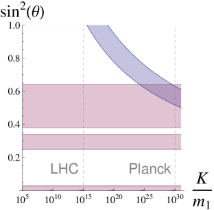
Figure 1: The parameter space $(K/m_{1},\sin^{2}\theta)$ is plotted. In blue, the acceptance region for the condition (22) (boundaries of the region correspond to $lhs=0.9$ and $lhs=1.1$). Physical mixing angles for three generation of neutrinos are: $\sin^{2}\theta_{13}=0.000^{+0.028}$, $\sin^{2}\theta_{12}=0.30^{+0.04}_{-0.05}$, $\sin^{2}\theta_{23}=0.50^{+1.4}_{-1.2}$ (within $2\sigma$) Giunti:2007ry. These values are also plotted in the graph (red regions). Dotted lines represents LHC energy scale ($\sim 1TeV$) and the Planck energy scale ($\sim 10^{28}eV$) fixing $m_{1}=10^{-2}eV$.

Focusing now on the latter of (II.4), we shall proceed with a similar analysis in order to test the hypothesis that the fermionic sector of the model provides a sensible Dark Matter candidate. As explained in the previous section, under the assumption that the flavour vacuum behaves as a perfect classical fluid on large scales, the fermionic contribution would get diluted with time as the universe expands. Its value today would then be

$$\rho_{f}(t_{now})=\rho_{f}\;\;a_{0}^{3}$$ (23)

with $a_{0}$ the scale factor corresponding to the time at which the model became effective. In order to reproduce the relation $(\Delta m^{2})\sim\rho_{f}(t_{now})$ we expect

$$a_{0}^{3}\frac{\sin^{2}\theta}{\pi^{2}}g(K/m_{1})\sim 1$$ (24)

that can be obtained by combining (23), (21) and (II.4). Because of the constrain on the Dark Energy density (22) the above condition becomes

$$a_{0}^{3}\frac{g(K/m_{1})}{f(K/m_{1})}\sim 1.$$ (25)

We already know that $a_{0}$ must be extremely small, but what is the ratio between $g(K/m_{1})$ and $f(K/m_{1})$ for large $K/m_{1}$ ($K/m_{1}>10^{14}$)?

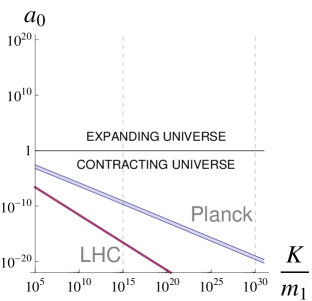
Figure 2: The parameter space $(K/m_{1},a_{0})$ is plotted. In blue, the acceptance region for the condition (22) (boundaries of the region correspond to $lhs=10$ and $lhs=0.1$). The red line depicts the scale factor of the real universe as a function of its average temperature, fixing $m_{1}=10^{-2}eV$. In a more realistic theory, the acceptance region (which may differ from the one here presented) is further reduced by comparison of the first of (II.4) with Dark Energy data, which gives a constraint on possible momentum cutoffs; the model is ruled out if the resulting region lies below the red line, since it would predict an amount of Dark Matter greater than what is observed; the model is consistent with data on Dark Matter if the region overlaps or lies above the red line; in this latter case the flavour vacuum contributes only to a fraction of total Dark Matter density.

As shown in Figure 2, equation (25) is indeed satisfied for large values of $K$ and very small values of $a_{0}$, as one would expect from a realistic theory. If, for instance, the cutoff is set equal to the Planck scale, relation (25) is satisfied for $a_{0}=10^{-20}$, which sets the transition phase (when the flavour vacuum became effective) well far in the past, when our toy universe was $10^{20}$ times smaller than “now”. Once more, parameters characterized by very different values ($a_{0}\sim 10^{-20}$, $K/m_{1}\sim 10^{30}$) combine together to give rise to a third scale, which has a physical significance (nowadays Dark Matter density).

Despite the unrealistic nature of our toy model, these first quantitative tests go in the right direction and certainly motivate the study of more realistic models, which hopefully will share with our toy model all the good features here discussed.

III Towards Interactive Flavour Vacua

III.1 A new method of calculation: Free WZ Revised

Following the standard literature, the results in Mavromatos:2010ni discussed so far have been derived by the following approach:

1. stress-energy tensor has been written in terms of massive fields;

2. massive fields have been decomposed in terms of massive ladder operators;

3. massive ladder operators have been written in terms of flavour ladder operators;

4. hence, stress-energy tensor has been written in terms of flavour ladder operators;

5. flavour-vev of the stress-energy tensor has been reduced by acting with the flavour ladder operators on the flavour vacuum.

However, such a long procedure can be avoided and the same exact result may be obtained in a much shorter way, following the steps:

1. flavour vacuum is written as $|0\rangle_{f}=G^{\dagger}_{\theta}|0\rangle$, the flavour-vev of $T_{\mu\nu}$ becoming a vev of $\mathcal{O}\equiv G_{\theta}T_{\mu\nu}G^{\dagger}_{\theta}$;

2. the stress-energy operator is transformed under the action of the $G_{\theta}{\color[rgb]{220,220,220}\blacksquare}G^{\dagger}_{\theta}$, using (3); the transformed operator $\mathcal{O}$ will be expressed in terms of the flavour fields, rather then the massive ones;

3. (I) is used to write the flavour fields in terms of the massive fields; $\mathcal{O}$ is again expressed in terms of the massive fields, but this time the operator $G_{\theta}$, and its complicated exponential structure, is not present any more;

4. a vev of $\mathcal{O}$, expressed as a simple combination of massive fields, is left, which can be reduced by decomposing the massive fields into massive ladder operators.

As a neat example of the above procedure, we will derive the results of Section II.1 via this new method. Recalling the discussion in Section II.1, in the study of the free WZ model we can consider the bosonic and the fermionic component separately, by evaluating relevant quantities in two separated contexts (a bosonic theory and a fermionic one) and eventually combining together the results. Furthermore, the pseudoscalar and the scalar field are indistinguishable for our purposes, therefore we are allowed to consider just the scalar field, keeping in mind to sum its contribution to the relevant quantities twice.

In the real scalar case, we have

$$T^{b}_{00}(x)=\sum_{i}\left(\pi_{i}^{2}(x)+\left(\vec{\nabla}\phi_{i}(x)\right)^{2}+m_{i}^{2}\phi_{i}^{2}(x)\right)$$ (26)

with $\pi_{i}\equiv\dot{\phi}_{i}$, the conjugate momentum of $\phi_{i}$. Since

$$G_{\theta}(t)=e^{i\theta\int d\vec{x}\left(\pi_{2}(x)\phi_{1}(x)-\pi_{1}(x)\phi_{2}(x)\right)}$$ (27)

from which

$$\begin{split}G_{\theta}(t)\phi_{1}(x)G^{\dagger}_{\theta}(t)=\phi_{1}(x)\cos\theta-\phi_{2}(x)\sin\theta\\ G_{\theta}(t)\phi_{2}(x)G^{\dagger}_{\theta}(t)=\phi_{1}(x)\sin\theta+\phi_{2}(x)\cos\theta\end{split}$$ (28)

and

$$\begin{split}G_{\theta}(t)\pi_{1}(x)G^{\dagger}_{\theta}(t)=\pi_{1}(x)\cos\theta-\pi_{2}(x)\sin\theta\\ G_{\theta}(t)\pi_{2}(x)G^{\dagger}_{\theta}(t)=\pi_{1}(x)\sin\theta+\pi_{2}(x)\cos\theta\end{split}$$ (29)

via the Baker-Campbell-Hausdorff formula

$$e^{Y}Xe^{-Y}=X+[Y,X]+\frac{1}{2}[Y,[Y,X]]+\frac{1}{3!}[Y,[Y,[Y,X]]]+...$$ (30)

we can write

$$G_{\theta}(t)\left(\sum_{i=1,2}\pi_{i}^{2}(x)\right)G_{\theta}^{\dagger}(t)=\left(\sum_{i=1,2}\pi_{i}^{2}(x)\right),$$ (31)

$$G_{\theta}(t)\left(\sum_{i=1,2}\left(\vec{\nabla}\phi_{i}(x)\right)^{2}\right)G_{\theta}^{\dagger}(t)=\\ \left(\sum_{i=1,2}\left(\vec{\nabla}\phi_{i}(x)\right)^{2}\right)$$ (32)

and

$$\langle 0|G_{\theta}(t)(m_{1}^{2}\phi_{1}^{2}(x)+m_{2}^{2}\phi_{2}^{2}(x))G_{\theta}^{\dagger}(t)|0\rangle=\\ \langle 0|(m_{1}^{2}\phi_{1}^{2}(x)+m_{2}^{2}\phi_{2}^{2}(x))|0\rangle+\\ \sin^{2}\theta(m_{1}^{2}-m_{2}^{2})\langle 0|(\phi_{2}^{2}(x)-\phi_{1}^{2}(x))|0\rangle.$$ (33)

It follows that

$${}_{f}\langle 0|T_{00}(x)|0\rangle_{f}=\langle 0|T_{00}(x)|0\rangle+\\ +\sin^{2}\theta(m_{1}^{2}-m_{2}^{2})\langle 0|(\phi_{2}^{2}(x)-\phi_{1}^{2}(x))|0\rangle$$ (34)

and therefore

$$\rho_{b}=_{f}\langle 0|:T_{00}(x):|0\rangle_{f}=\\ =\sin^{2}\theta(m_{1}^{2}-m_{2}^{2})\langle 0|(\phi_{2}^{2}(x)-\phi_{1}^{2}(x))|0\rangle$$ (35)

Equivalently for $T_{jj}(x)$ we have

$$\mathsf{P}_{b}=_{f}\langle 0|:T_{jj}(x):|0\rangle_{f}=-\sin^{2}\theta(m_{1}^{2}-m_{2}^{2})\times\\ \times\langle 0|(\phi_{2}^{2}(x)-\phi_{1}^{2}(x))|0\rangle=-\rho_{b}.$$ (36)

Once the fields in (35) and (36) are decomposed in terms of the ladder operators and the quantum algebra is simplified, expressions (15) and (16) are correctly reproduced.

In the fermionic case, a similar procedure leads to

$$\rho_{f}=_{f}\langle 0|:T_{00}^{f}(x):|0\rangle_{f}=\sin^{2}\theta\left(m_{1}-m_{2}\right)\times\\ \times\langle 0|\left(\bar{\psi}_{2}(x)\psi_{2}(x)-\bar{\psi}_{1}(x)\psi_{1}(x)\right)|0\rangle$$ (37)

and

$$\mathsf{P}_{f}=_{f}\langle 0|:T_{jj}^{f}(x):|0\rangle_{f}=0.$$ (38)

By comparing (37) and (35), the analogy between the fermionic and the bosonic condensate that earlier was hidden in formulae (15) and (16) is now more evident. Again, formula (16) is correctly reproduced, once the operatorial structure of the fields is simplified with respect to $\langle 0|{\color[rgb]{220,220,220}\blacksquare}|0\rangle$. The expression (37) dispels any doubts concerning formula (16) and its possible dependency on the specific form of the gamma matrices and spinors used to achieve the results of Mavromatos:2010ni, being (37) independent of such a choice Peskin:1995ev.

Furthermore, Supersymmetry enables us to rewrite this result in terms of the bosonic fields only. For the massive vacuum $|0\rangle$ we know that

$$\langle 0|T_{\mu\nu}(x)|0\rangle=0$$ (39)

which leads to

$$\langle 0|\bar{\psi}_{i}(x)\psi_{i}(x)|0\rangle=-4m_{i}\langle 0|\phi^{2}_{i}(x)|0\rangle$$ (40)

and hence

$$\rho_{WZ}=2\sin^{2}\theta(m_{1}-m_{2})^{2}\langle 0|\left(\phi_{1}^{2}(x)+\phi_{2}^{2}(x)\right)|0\rangle$$ (41)

$$\mathsf{P}_{WZ}=-2\sin^{2}\theta(m_{1}^{2}-m_{2}^{2})\langle 0|(\phi_{2}^{2}(x)-\phi_{1}^{2}(x))|0\rangle$$ (42)

in accordance with (13) and (14).

The procedure exemplified in the previous section can be easily implemented for other fields: one might want to consider Dirac or two component Weyl spinors as well as complex scalar fields, getting to analogous results. For mere speculative reasons, applications to vector fields or even more complex objects might be thought: the method involves a manipulation of the stress-energy tensor, with the use of equation of motion of the field and its (anti-)commutation rules, regardless of the tensorial or spinorial structure of the field itself. Furthermore, extending these results to more then two flavours is rather straightforward.

Finally, the method enables us to distinguish among all the terms of the stress-energy tensors the ones that really contribute to the final result. This might be helpful in understanding the behaviour of the flavour vacuum in more realistic theories, as we shall see in the forthcoming sections.

III.2 Self-interactive Bosons

An example of the applications just discussed is offered by a $\lambda\phi^{4}$ model. The theory

$$\mathcal{L}=\sum_{i=1,2}\left(\partial_{\mu}\phi_{i}\partial^{\mu}\phi_{i}-m_{i}^{2}\phi_{i}^{2}-\lambda\phi_{i}^{4}\right)$$ (43)

can be regarded as derived from a model with flavour mixing:

$$\mathcal{L}=\partial_{\mu}\phi_{A}\partial^{\mu}\phi_{A}+\partial_{\mu}\phi_{B}\partial^{\mu}\phi_{B}-m_{A}^{2}\phi_{A}^{2}-m_{B}^{2}\phi_{B}^{2}+\\ -m_{AB}^{2}\phi_{A}\phi_{B}-\!\!\!\!\!\!\!\!\sum_{\iota,\kappa,\lambda,\rho=A,B}\!\!\!\!\!\!\!\!g_{\iota\kappa\lambda\rho}\phi_{\iota}\phi_{\kappa}\phi_{\lambda}\phi_{\rho}$$ (44)

with the usual rotation

$$\begin{split}\phi_{A}=\cos\theta\phi_{1}-\sin\theta\phi_{2}\\ \phi_{B}=\sin\theta\phi_{1}+\cos\theta\phi_{2}\end{split}$$ (45)

and a specific choice of the coupling constants $g_{{\color[rgb]{220,220,220}\blacksquare}}$. Since the expression of $G_{\theta}$ in terms of the fields can be deduced from

$$\begin{split}G_{\theta}^{\dagger}\phi_{1}G_{\theta}=\cos\theta\phi_{1}-\sin\theta\phi_{2}\\ G_{\theta}^{\dagger}\phi_{2}G_{\theta}=\sin\theta\phi_{1}+\cos\theta\phi_{2}\end{split}$$ (46)

just using commutation relations between fields and conjugate momenta, which are not modified by the form of the Lagrangian Peskin:1995ev, expression

$$G_{\theta}=e^{i\theta\int d\vec{x}(\dot{\phi}_{2}\phi_{1}-\dot{\phi}_{1}\phi_{2})}$$ (47)

that was found valid in the free case, holds also in the interactive one.

If we assume that the flavour vacuum is defined as

$$|0\rangle_{f}\equiv G^{\dagger}_{\theta}|0\rangle$$ (48)

naïvely generalizing the free case, with $|0\rangle$ the ground state of the theory described by (43), we can easily see that

$${}_{f}\langle 0|T_{\mu\nu}|0\rangle_{f}=\langle 0|T_{\mu\nu}|0\rangle+\\ +\eta_{\mu\nu}\left(\sin^{2}\theta(m_{1}^{2}-m_{2}^{2})\langle 0|\phi_{2}^{2}-\phi_{1}^{2}|0\rangle\right)+\\ +\eta_{\mu\nu}\lambda\langle 0|\left((\phi_{2}\cos(\theta)-\phi_{1}\sin(\theta))^{4}+\right.\\ +\left.(\phi_{1}\cos(\theta)+\phi_{2}\sin(\theta))^{4}-\phi_{1}^{4}-\phi_{2}^{4}\right)|0\rangle.$$ (49)

We can therefore state that the equation of state is given by

$$w=\frac{{}_{f}\langle 0|:T_{jj}:|0\rangle_{f}}{{}_{f}\langle 0|:T_{00}:|0\rangle_{f}}=\\ =\frac{-\langle 0|\because\sum_{i=1,2}(m_{i}^{2}\phi_{i}^{2}+\lambda\phi_{i}^{4})\because|0\rangle}{\langle 0|\because\sum_{i=1,2}(m_{i}^{2}\phi_{i}^{2}+\lambda\phi_{i}^{4})\because|0\rangle}=-1$$ (50)

in which

$$\because f(\varphi_{1},\varphi_{2})\because\equiv\\ f(\cos\theta\varphi_{1}-\sin\theta\varphi_{2},\sin\theta\varphi_{1}+\cos\theta\varphi_{2})-f(\varphi_{1},\varphi_{2}).$$ (51)

Quite notably, this result generalizes the analogous result for the free theory, in a completely non-perturbative way: equation (50) is independent of the explicit form of the fields and the ground state $|0\rangle$, which we might be able to recover just in a perturbative treatment of the model.

In fact, it is possible the further generalize the above result for any interactive theory for two scalar fields with flavour mixing in the following form:

$$\mathcal{L}=\partial_{\mu}\phi_{A}\partial^{\mu}\phi_{A}+\partial_{\mu}\phi_{B}\partial^{\mu}\phi_{B}-m_{A}^{2}\phi_{A}^{2}-m_{B}^{2}\phi_{B}^{2}+\\ -m_{AB}^{2}\phi_{A}\phi_{B}+\mathcal{L}_{int}(\phi_{A},\phi_{B})$$ (52)

with $\mathcal{L}(\phi_{A},\phi_{B})$ any polynomial function of $\phi_{A}$ and $\phi_{B}$. It is easy to show that

$${}_{f}\langle 0|:T_{\mu\nu}:|0\rangle_{f}=\eta_{\mu\nu}\langle 0|\because\sum_{i=1,2}m_{i}^{2}\phi^{2}_{i}-\mathcal{L}_{int}\because|0\rangle$$ (53)

leading always to the equation of state $w=-1$.

III.3 Self-interactive fermions

Analogously, we can generalize the result presented in Section II.1 for fermionic fields (namely, $w=0$) for a certain class of self-interactive theories. We start by considering a theory written in terms of the massive fields $\psi_{1}$ and $\psi_{2}$:

$$\mathcal{L}=\sum_{i}\bar{\psi}_{i}(i\partial\!\!\!/-m_{i})\psi_{i}+\mathcal{L}_{int}$$ (54)

with $\mathcal{L}_{int}$ a suitable polynomial function of $\psi_{i}$ and $\bar{\psi}_{i}$. Again, we regard (54) as the diagonalized Lagrangian: in case of flavour mixing, $\psi_{1}$ and $\psi_{2}$ come from a rotation of the flavoured fields $\psi_{A}$ and $\psi_{B}$.

Combining our previous discussion on the bosonic case and results of Section III.1, we can write rCl_f⟨0 —: T_00 : —0⟩_f&= ⟨0 —∵T_00 ∵— 0 ⟩ =
=⟨0 —∵∑_i m_i ¯ψ