Oscillation mode linewidths of main-sequence and subgiant stars observed by Kepler

Abstract

Context. Solar-like oscillations have been observed by Kepler and CoRoT in several solar-type stars.

Aims. We study the variations of stellar p-mode linewidth as a function of effective temperature.

Methods. Time series of 9 months of Kepler data have been used. The power spectra of 42 cool main-sequence stars and subgiants have been analysed using both Maximum Likelihood Estimators and Bayesian estimators, providing individual mode characteristics such as frequencies, linewidths and mode heights.

Results. Here we report on the mode linewidth at maximum power and at maximum mode height for these 42 stars as a function of effective temperature.

Conclusions. We show that the mode linewidth at either maximum mode height or maximum amplitude follows a scaling relation with effective temperature, which is a combination of a power law plus a lower bound. The typical power law index is about 13 for the linewidth derived from the maximum mode height, and about 16 for the linewidth derived from the maximum amplitude while the lower bound is about 0.3 $\mu$Hz and 0.7 $\mu$Hz, respectively. We stress that this scaling relation is only valid for the cool main-sequence stars and subgiants, and does not have predictive power outside the temperature range of these stars.

1 Introduction

Stellar physics faces a revolution following the great wealth of asteroseismic data made available by space missions such as CoRoT (Baglin, 2006) and Kepler (Borucki et al., 2009). Long observations of solar-like pulsators corresponding to main sequence stars, subgiants and red giants have been performed during more than 6 months by CoRoT (Baudin et al., 2011a, b, and references therein). The Kepler mission now provides a larger sample of stars observed for longer durations (Chaplin et al., 2011).

The study of oscillation mode physics (mode height, linewidth and amplitude) provides information on excitation and damping mechanisms related to the physics of convection and of stellar atmospheres (Samadi, 2009). Houdek et al. (1999) theoretically derived stellar mode linewidths as a function of stellar mass and age. They found that stellar mode linewidths would present a depression or plateau close to the maximum of mode height. This depression was first detected in the solar p-mode linewidths by Fröhlich et al. (1995). Such a depression is due to a resonance between the thermal adjustment time of the superadiabatic boundary layer and the mode frequency (Balmforth, 1992). The frequency location of the maximum of mode height is in turn related to the Mach number (${\cal M}_{a}$), the ratio of convective velocity to the sound speed (Belkacem et al., 2011). The convective flux giving the maximum mode amplitude is also related to ${\cal M}_{a}$ to the power of 3 (e.g. Belkacem et al., 2011; Houdek et al., 1999). It is therefore interesting to study how the mode linewidth is related to the frequency of maximum amplitude / mode height for several different stars.

Statistical studies over a large number of stars have been performed in order to validate the scaling relation derived for the amplitude of stellar oscillations by Kjeldsen & Bedding (1995) and recently revised by Kjeldsen & Bedding (2011). Scaling relations for mode linewidth have been proposed by Chaplin et al. (2009) and Baudin et al. (2011a) based upon the stellar effective temperature.

Chaplin et al. (2009) proposed a scaling relation with linewidth proportional to $T_{\rm eff}^{4}$ based upon several ground-based observations. Using CoRoT observations, Baudin et al. (2011b) measured linewidths for a sample of solar-like pulsators and provided a scaling relation proportional to $T_{\rm eff}^{16}$.

With the ability to perform longer observations of stars with Kepler, the measurement of mode linewidth becomes easier and more reliable. In this paper, based upon Kepler observations and using a larger stellar sample than of Baudin et al. (2011a), we derive a new relation between mode linewidth and $T_{\rm eff}$ .

2 Data analysis

2.1 Time series and power spectra

Kepler observations are obtained in two different operating modes: long cadence (LC) and short cadence (SC) (Gilliland et al., 2010; Jenkins et al., 2010). This work is based on SC data. For the brightest stars (down to Kepler magnitude, $Kp\approx 12$), SC observations can be obtained for a limited number of stars (up to 512 at any given time) with a faster sampling rate of 58.84876 s (Nyquist frequency of $\sim$ 8.5 mHz), allowing for more precise transit timing. The time series were corrected for outliers, occasional jumps and drifts (see García et al., 2011), and the levels between the quarters were normalized. Finally, the resulting light curves have been high-pass filtered using a triangular smoothing of width 1 day, to minimize the effects of the long period instrumental drifts. The power spectra were produced from a single source using the Lomb-Scargle periodogram (Scargle, 1982), properly calibrated to comply with Parseval’s theorem (see Appourchaux, 2011).

Kepler observations are divided into three-month-long Quarters (Q). A subset of 42 cool main-sequence stars and subgiants observed during quarters Q5, Q6 and Q7 (March 22, 2010 to December 22, 2010) were chosen for having oscillation modes with high signal-to-noise ratios ranging from 1.8 to 50 in the power spectrum. The frequency resolution is about 0.04 $\mu$Hz. Figure 1 shows the measured large frequency separation of these 42 stars as a function of their effective temperature provided by Pinsonneault et al. (2011). The large separation is derived from individual mode frequencies at $\nu_{\rm max}$ from the All data set (See Table 1.). We took care to analyse solar-type stars without avoided crossings, since these may reduce the observed linewidths. The avoided crossings were detected by visual inspection of the echelle diagram; examples of such avoided crossings can be found in Deheuvels et al. (2010); Metcalfe et al. (2010); Mathur et al. (2011); Campante et al. (2011); Bedding (2011).

Figure 1: Large separation as a function of effective temperature of the stars used in this study. The error bars on the large separations are within the thickness of the symbol. The evolutionary tracks for stars of mass 0.8 M_⊙(most right) to 1.5 M_⊙ (most left) (by step of 0.1 M_⊙) are shown as dotted lines. The tracks are derived from Marigo et al. (2008).

2.2 Mode parameter extraction

The mode parameter extraction was performed by 11 fitters. The list of fitted modes were compared for completeness and 5 fitters were selected for finalising the parameters: two fitters (IAS, BIR), who applied maximum likelihood estimators (MLE), and three Bayesian fitters (SYD, MAR and AAU).

The power spectra were modelled over a frequency range covering typically about 15 to 20 large separations (=$\Delta\nu$). For each radial order, the model parameters were mode frequencies (one each for $l$=0,1,2), a single mode height (with an assumed ratio of $H_{1}/H_{0}=1.5$, $H_{2}/H_{0}$=0.5) and a single mode linewidth. In the case of AAU only, the $l=0$ linewidths were fitted and the linewidths of the other degrees were interpolated in between two $l=0$ mode linewidths. The relative heights $H_{(l,m)}$ of the split components of the modes depend on the stellar inclination angle as given by Gizon & Solanki (2003). For each star, the rotational splitting and stellar inclination angle were chosen to be common across all the modes. The mode profile was assumed to be Lorentzian. The background was modelled using a multi-component Harvey model (Harvey, 1985) with two parameters and a white noise component. We used a single Harvey component for all stars, and a double component for 11 stars (BIR’s stars). In total the number of free parameters for 15 orders was at least $5\times 15+2=77$.

The two models described above were used for fitting the parameters of the stars using MLE. All 42 stars were fitted by IAS, 16 of which were fitted by IAS alone. Eleven stars were fitted by BIR. The fit was done without and with rotational splitting; the significance of splitting and angle was then tested using the likelihood ratio test, by applying the H₀ hypothesis with a cutoff for a $\chi^{2}$ with 2 d.o.f of $\Delta{\log}({\rm likelihood})$=9.2 (4.6) or a probability of 10^-4 (10^-2) for IAS, and for BIR, respectively. Formal uncertainties on each parameter were derived from the inverse of the Hessian matrix (for more details on MLE, significance and formal errors, see Appourchaux, 2011).

Fifteen stars with large mode linewidths were fitted with a Bayesian approach using different sampling methods. SYD and AAU employed MCMC (Benomar et al., 2009; Handberg & Campante, 2011), while MAR used nested sampling via the code MultiNest (Feroz et al., 2009). For the nested sampling approach, the large number of parameters forced us to use MultiNest’s constant efficiency, mono-modal mode. The priors on the central frequency and inclination angle were uniform. The prior on the splitting was either uniform from 0-10 $\mu$Hz (MAR) or a combination of a uniform prior over 0-2 $\mu$Hz and a decaying Gaussian (SYD, AAU). The priors on mode height were modified Jeffreys priors (Benomar et al., 2009; Gruberbauer et al., 2009), and the priors on the linewidth were either uniform (MAR) or modified Jeffreys priors (SYD, AAU). The error bars were derived from the marginal posterior distribution of each parameter. Each Bayesian fitter had 7 stars to fit: 4 stars + 3 common stars. The latter are used for comparison of the Bayesian methods. Priors on frequencies were set after visual inspection of the power spectrum. Modes of degree $l=2$ were assumed to be on the low-frequency side of the $l=0$ (i.e., the small spacing $d_{02}$ is assumed positive). In order to avoid spurious results, one of the Bayesian fitters (SYD) also used a smoothness condition on the frequency for each degree.

The different data sets available are summarized in Table 1.

Table 1: Data set of fitted stars.

Dataset	Fitter	Method	# of stars	Comment
I	IAS	MLE	16	No common stars
II	BIR	MLE	11	No common stars
III	SYD	Bayes	7	Common stars$\dagger$
IV	MAR	Bayes	7	Common stars$\dagger$
V	AAU	Bayes	7	Common stars$\dagger$
All	IAS	MLE	42	All stars included

$\dagger$From these, 3 stars commonly fitted by SYD, MAR and AAU

2.3 Linewidths

In a similar fashion to Baudin et al. (2011a), we derived the mean linewidth ($\Gamma_{\nu_{\rm max}}$) at maximum mode height and at maximum mode amplitude by taking the weighted average of 3 linewidths of 3 orders around the frequency of these maxima (See Tables 4 and 5 as online materials). The derivation of $\Gamma_{\nu_{\rm max}}$ is rather immune to systematic effects resulting from the 3-mode average because at these frequencies the observed linewidths exhibit a plateau, as shown theoretically by Houdek et al. (1999) and as observed in the Sun by Fröhlich et al. (1995).

Individual mode linewidths can have systematic errors resulting from the incorrect estimation of several mode profile parameters. In addition, an over- or underestimation of mode linewidths will provide an under- or overestimation of mode heights, respectively. Estimates of such systematic errors can be derived using the procedure developed by Toutain et al. (2005), which consists in fitting one model profile, without using Monte-Carlo simulations.

The main parameters producing systematic errors on mode linewidths are: the background noise $B$, the mode height ratio and the splitting.

The major source of systematic errors on mode height and mode linewidth is the biased estimation of the background noise. An estimate of the mode linewidth bias can be derived for a single mode using the analytical formulae provided by Toutain & Appourchaux (1994). We can then derive the bias on mode linewidth as a function of the error on $\Delta B$ and the inverse signal-to-noise ratio ($\beta=B/H$) in the power spectrum:

$$\frac{\Delta\Gamma}{\Gamma}=k(\beta,\Gamma,\Delta\nu)\frac{\Delta B}{B}\leavevmode\nobreak\ ,$$ (1)

where $\Delta\nu$ is the window over which the fit is performed for that single mode. Typically $k$ is negative and of order 1, i.e., under-estimation of the background by 10 % will lead to an over-estimation of the linewidth by 10%. Another source of systematic errors is the assumption that the ratios of mode height be fixed to some given values. There is indeed a variation of mode height ratios with effective temperature as shown by Ballot et al. (2011). The resulting underestimation of these ratios is typically not larger than 0.1, which corresponds roughly to an underestimation of the linewidths not larger than 3%. A minor source of systematic errors comes from the rotational splitting. In the case for which the splitting is not detected (typically when the splitting is not greater than 10 % of the linewidth), the linewidth will be overestimated by about 6% for $\Gamma\leavevmode\nobreak\ =10\leavevmode\nobreak\ \mu$Hz, and by about 3% for $\Gamma\leavevmode\nobreak\ =\leavevmode\nobreak\ 3\leavevmode\nobreak\ \mu$Hz. When the splitting is larger, there is no correlation between the detected splitting and the linewidth (Toutain & Appourchaux, 1994). All these values were either confirmed or inferred with the procedure suggested by Toutain et al. (2005).

Last but not least, an extrinsic systematic effect on the linewidth is related to stellar activity. It was shown by Chaplin et al. (2000), that the solar linewidth may change by typically 20% at the location of the dip. We are aware that this can have an effect on the mean linewidth reported here. For many stars, this effect cannot be assessed with such a short observation duration of 9 months.

3 Discussion

Figure 2 shows the linewidth measured at maximum mode height as a function of effective temperature. We note that Chaplin et al. (2009) proposed a scaling relation, which provides a variation of the mode linewidth by a factor 2.7 between 6800 K and 5300 K; while Baudin et al. (2011b) provides a factor of 53.9 for the same temperature change. The measured ratio, here, is closer to 10. It is clear that neither dependence is adequate to explain our measurements. The results of Chaplin et al. (2009) were based on predicted mode lifetimes from pulsation computations, and also on a small number of relatively short ground-based observations, potentially subject to large systematic errors.

We tested three forms of the $T_{\rm eff}$ relations, namely an exponential variation, a pure power law, and a power law with a flat component. Without any physical basis for choosing between the different relations, we adopted the one with the lowest $\chi^{2}$, which was the third of these:

$$\Gamma=\Gamma_{0}+\alpha\left(\frac{T_{\rm eff}}{5777}\right)^{s}\leavevmode\nobreak\ .$$ (2)

The effective temperatures were derived from two re-calibrations of the photometry in the Kepler Input Catalog: one based on $griz$ use of the photometry (Pinsonneault et al., 2011) and one based on application of the Infrared Flux Method using 2MASS $JHK$ (Casagrande et al., 2010, 2006). The random errors on the fitted parameters were derived using Monte-Carlo simulations of the fit taking into account random errors on both the effective temperature and the linewidths.

Tables 2 and 5 give the results of the fitted parameters of the linewidth at $\nu_{\rm max}$ for the two different effective temperatures and the two different ways of measuring $\nu_{\rm max}$. This latter can be derived either from the maximum of the mode amplitude, which is $\propto E$ (where $\sqrt{E}$ is the energy injected by convection) or from the maximum of mode height, which is $\propto E/\Gamma$. We used five different sets of linewidth data to study the impact of the different method upon the fitted parameters: all fitted linewidth (MLE and Bayesian), all fitted linewidth (excluding either BIR or IAS’s), MLE (fitted by IAS and BIR only), MLE (fitted only by IAS).

Here we note that the power law indices are rather close to the index given by Baudin et al. (2011b) (See Table 2). The mode linewidth measured at the maximum mode height is systematically lower on average by about 10% than that measured at the maximum amplitude. This is because the frequency of maximum amplitude tends to be higher than the frequency of maximum mode height.

The different power law index between the two sources of effective temperature is mainly due to the fact that the range of temperature is smaller for Pinsonneault et al. (2011) compared to Casagrande et al. (2010); the reduction is 75 K, mainly at the high temperatures. The lower temperature range would increase $s$ by 1.0 and 1.5, which is roughly in agreement with Tables 2 and 5, respectively.

We also studied the impact of having different fitters upon the derived parameters. From Tables 2 and 5, we can see that the fitted parameters are the same within error bars when we combine the MLE fits with the Bayesian fits. There is a much larger difference when we use the linewidth derived on all stars by IAS only (the only homogenous data set), thereby also including the stars for which the effective temperature is higher than 6400 K. For that homogenous data set, the linewidths measured at high effective temperature are systematically higher than those measured by the Bayesian fitters by up to 15%. Typically, a change of the linewidth at the highest effective temperature of 1 $\mu$Hz will increase $s$ by 1. The sensitivity of the power law index $s$ to the high effective temperatures also explains why the index does not vary much when other data sets obtained at lower effective temperature are included (The data sets I and II from the MLE fitters are at low effective temperature).

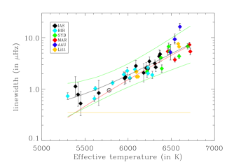
Figure 2: Average mode linewidth at maximum mode height (and their 3-$\sigma$ error bars) as a function of effective temperature (provided by Pinsonneault et al., 2011). The error bars on the effective temperatures although not shown here are indeed included in the error analysis. Average mode linewidth fitted by IAS (black), by BIR (cyan), by SYD (green), by MAR (red), by AAU (blue), from Baudin et al. (2011a) (orange). Fitted average linewidth (Black line). 3-$\sigma$ error bars on fitted average linewidth (Green lines). Power law component of the fit (Red line). Flat component at low $T_{\rm eff}$ (Orange line). The mean mode linewidth of the Sun is indicated at 5777 K.

Table 2: Parameters of the fit of Eq. (2) and their random errors for linewidth measured at maximum mode height.

Dataset	$T_{\rm eff}$	$\Gamma_{0}$ ($\mu$Hz)	$\alpha$ ($\mu$Hz)	s
I+II+III+IV+V	Pins.	0.35 $\pm$ 0.13	0.91 $\pm$ 0.16	13.7 $\pm$ 1.4
I+II$\dagger$	Pins.	0.32 $\pm$ 0.17	0.93 $\pm$ 0.20	12.7 $\pm$ 2.1
All	Pins.	0.46 $\pm$ 0.09	0.75 $\pm$ 0.11	15.4 $\pm$ 1.3
I+II+III+IV+V	Casa.	0.20 $\pm$ 0.14	0.97 $\pm$ 0.17	13.0 $\pm$ 1.4

$\dagger$Range for these stars is 5300 K to 6400 K

Table 3: Parameters of the fit of Eq. (2) and their random errors bars for linewidth measured at maximum mode amplitude.

Dataset	$T_{\rm eff}$	$\Gamma_{0}$ ($\mu$Hz)	$\alpha$ ($\mu$Hz)	s
I+II+III+IV+V	Pins.	0.64 $\pm$ 0.11	0.66 $\pm$ 0.14	16.7 $\pm$ 1.8
I+II$\dagger$	Pins.	0.65 $\pm$ 0.10	0.64 $\pm$ 0.13	16.1 $\pm$ 2.3
All	Pins.	0.65 $\pm$ 0.09	0.64 $\pm$ 0.10	17.0 $\pm$ 1.4
I+II+III+IV+V	Casa.	0.49 $\pm$ 0.12	0.75 $\pm$ 0.15	15.5 $\pm$ 1.6

$\dagger$Range for these stars is 5300 K to 6400 K

4 Conclusion

We studied the dependence of linewidth at maximum mode height and amplitude on $T_{\rm eff}$ for two sources effective temperature and for two ways of deriving the linewidth. We showed using 9 months of Kepler observations of 42 stars that the mode linewidth at both maximum mode height or maximum amplitude follows a scaling relation based on effective temperature, which is a combination of a power law plus a lower bound. We stress that this scaling relation is only valid for the cool main-sequence and subgiant stars, and does not have predictive power outside the temperature range of these stars.

Table 4: Natural logarithm of the linewidth measured at maximum mode height with their error bars for each star, together with the frequency of the maximum, the effective temperature of Pinsonneault et al. (2011) and of Casagrande et al. (2010, 2006), with their respective error bars.

KIC number	$T_{\rm eff}^{\rm Pins}$	$T_{\rm eff}^{\rm Cas}$	$\nu_{\rm max}$	$\gamma$ ($\ln\mu$Hz)	Fitter
1435467	6541 $\pm$ 126	6433 $\pm$ 58	1414.3	1.422 $\pm$ 0.073	IAS
2837475	6710 $\pm$ 61	6664 $\pm$ 92	1585.3	2.228 $\pm$ 0.072	IAS
3424541	6460 $\pm$ 55	6723 $\pm$ 83	678.8	1.480 $\pm$ 0.112	IAS
3427720	5970 $\pm$ 52	6100 $\pm$ 80	2684.6	0.542 $\pm$ 0.093	IAS
3733735	6720 $\pm$ 56	6827 $\pm$ 96	2026.9	2.227 $\pm$ 0.102	IAS
3735871	6220 $\pm$ 61	6298 $\pm$ 67	2747.4	1.012 $\pm$ 0.137	IAS
6116048	6020 $\pm$ 51	6073 $\pm$ 69	2150.0	0.420 $\pm$ 0.072	IAS
6508366	6480 $\pm$ 56	6379 $\pm$ 90	979.8	1.599 $\pm$ 0.074	IAS
6603624	5610 $\pm$ 51	5672 $\pm$ 58	2367.0	-0.423 $\pm$ 0.078	IAS
6679371	6590 $\pm$ 56	6473 $\pm$ 89	854.0	1.623 $\pm$ 0.062	IAS
6933899	5820 $\pm$ 50	5837 $\pm$ 73	1393.9	0.239 $\pm$ 0.065	IAS
7103006	6390 $\pm$ 56	6381 $\pm$ 84	1132.8	1.415 $\pm$ 0.080	IAS
7106245	6020 $\pm$ 51	6041 $\pm$ 69	2382.8	0.312 $\pm$ 0.182	IAS
7206837	6360 $\pm$ 56	6428 $\pm$ 75	1509.0	1.472 $\pm$ 0.095	IAS
7871531	5390 $\pm$ 47	5331 $\pm$ 42	3254.7	0.122 $\pm$ 0.146	IAS
8006161	5300 $\pm$ 46	5399 $\pm$ 41	3518.5	-0.354 $\pm$ 0.085	IAS
8228742	6080 $\pm$ 51	6235 $\pm$ 76	1126.9	0.824 $\pm$ 0.070	IAS
8379927	5990 $\pm$ 52	5965 $\pm$ 62	2684.0	0.815 $\pm$ 0.066	IAS
8394589	6210 $\pm$ 52	6276 $\pm$ 75	2328.6	0.942 $\pm$ 0.085	IAS
8694723	6310 $\pm$ 56	6401 $\pm$ 73	1435.3	1.148 $\pm$ 0.051	IAS
9025370	5660 $\pm$ 52	5737 $\pm$ 69	2848.3	-0.173 $\pm$ 0.188	IAS
9098294	5960 $\pm$ 51	5984 $\pm$ 60	2334.9	0.481 $\pm$ 0.089	IAS
9139151	6090 $\pm$ 52	6226 $\pm$ 78	2620.2	1.040 $\pm$ 0.084	IAS
9139163	6370 $\pm$ 56	6510 $\pm$ 90	1704.5	1.569 $\pm$ 0.055	IAS
9206432	6470 $\pm$ 56	6677 $\pm$ 109	1903.9	2.129 $\pm$ 0.086	IAS
9410862	6180 $\pm$ 51	6174 $\pm$ 65	2184.9	0.732 $\pm$ 0.137	IAS
9812850	6380 $\pm$ 55	6382 $\pm$ 95	1264.4	1.680 $\pm$ 0.078	IAS
9955598	5450 $\pm$ 47	5492 $\pm$ 45	3453.4	-0.642 $\pm$ 0.180	IAS
10018963	6230 $\pm$ 52	6154 $\pm$ 78	947.2	0.854 $\pm$ 0.052	IAS
10162436	6320 $\pm$ 53	6253 $\pm$ 77	1008.6	0.981 $\pm$ 0.064	IAS
10355856	6540 $\pm$ 56	6595 $\pm$ 77	1280.5	1.754 $\pm$ 0.079	IAS
10454113	6246 $\pm$ 58	6071 $\pm$ 74	2333.2	1.245 $\pm$ 0.066	IAS
10644253	6020 $\pm$ 51	6122 $\pm$ 69	2993.2	0.805 $\pm$ 0.137	IAS
10909629	6490 $\pm$ 61	6420 $\pm$ 73	893.1	1.220 $\pm$ 0.101	IAS
10963065	6280 $\pm$ 51	6177 $\pm$ 67	2195.5	0.822 $\pm$ 0.064	IAS
11081729	6600 $\pm$ 62	6696 $\pm$ 81	1803.2	1.887 $\pm$ 0.103	IAS
11244118	5620 $\pm$ 51	5824 $\pm$ 62	1383.7	-0.081 $\pm$ 0.077	IAS
11253226	6690 $\pm$ 56	6789 $\pm$ 99	1685.8	2.166 $\pm$ 0.056	IAS
11772920	5420 $\pm$ 51	5440 $\pm$ 44	3394.7	-0.241 $\pm$ 0.174	IAS
12009504	6230 $\pm$ 51	6337 $\pm$ 71	1870.5	0.628 $\pm$ 0.092	IAS
12258514	5950 $\pm$ 51	5967 $\pm$ 70	1517.1	0.515 $\pm$ 0.053	IAS
12317678	6540 $\pm$ 55	6558 $\pm$ 86	1201.9	1.594 $\pm$ 0.058	IAS
6116048	6020 $\pm$ 51	6073 $\pm$ 69	2150.0	0.507 $\pm$ 0.053	BIR
6603624	5610 $\pm$ 51	5672 $\pm$ 58	2367.0	-0.427 $\pm$ 0.042	BIR
6933899	5820 $\pm$ 50	5837 $\pm$ 73	1321.5	0.278 $\pm$ 0.031	BIR
8006161	5300 $\pm$ 46	5399 $\pm$ 41	3518.4	-0.312 $\pm$ 0.050	BIR
8228742	6080 $\pm$ 51	6235 $\pm$ 76	1189.0	0.884 $\pm$ 0.042	BIR
8379927	5990 $\pm$ 52	5965 $\pm$ 62	2684.0	0.820 $\pm$ 0.052	BIR
10018963	6230 $\pm$ 52	6154 $\pm$ 78	947.2	0.958 $\pm$ 0.033	BIR
10963065	6280 $\pm$ 51	6177 $\pm$ 67	2092.4	0.637 $\pm$ 0.054	BIR
11244118	5620 $\pm$ 51	5824 $\pm$ 62	1312.2	0.028 $\pm$ 0.031	BIR
12009504	6230 $\pm$ 51	6337 $\pm$ 71	1870.5	0.706 $\pm$ 0.069	BIR
12258514	5950 $\pm$ 51	5967 $\pm$ 70	1517.1	0.656 $\pm$ 0.040	BIR
3735871	6220 $\pm$ 61	6298 $\pm$ 67	2747.3	0.792 $\pm$ 0.088	SYD
6508366	6480 $\pm$ 56	6379 $\pm$ 90	980.0	1.678 $\pm$ 0.039	SYD
6679371	6590 $\pm$ 56	6473 $\pm$ 89	854.0	1.472 $\pm$ 0.032	SYD
7103006	6390 $\pm$ 56	6381 $\pm$ 84	1133.1	0.922 $\pm$ 0.056	SYD
9206432	6470 $\pm$ 56	6677 $\pm$ 109	1864.6	1.911 $\pm$ 0.051	SYD
9812850	6380 $\pm$ 55	6382 $\pm$ 95	1170.3	1.408 $\pm$ 0.050	SYD
11253226	6690 $\pm$ 56	6789 $\pm$ 99	1608.9	1.918 $\pm$ 0.040	SYD
1435467	6541 $\pm$ 126	6789 $\pm$ 99	1205.4	1.318 $\pm$ 0.036	MAR
2837475	6710 $\pm$ 61	6433 $\pm$ 58	1509.2	1.987 $\pm$ 0.039	MAR
3424541	6460 $\pm$ 55	6664 $\pm$ 92	677.8	1.688 $\pm$ 0.048	MAR
3733735	6720 $\pm$ 56	6723 $\pm$ 83	1655.4	1.685 $\pm$ 0.049	MAR
10355856	6540 $\pm$ 56	6595 $\pm$ 77	1280.4	2.242 $\pm$ 0.074	AAU
10909629	6490 $\pm$ 61	6420 $\pm$ 73	942.5	1.657 $\pm$ 0.118	AAU
11081729	6600 $\pm$ 62	6696 $\pm$ 81	1892.2	2.796 $\pm$ 0.052	AAU
12317678	6540 $\pm$ 55	6789 $\pm$ 99	1166.8	2.229 $\pm$ 0.053	AAU

Table 5: Natural logarithm of the linewidth measured at maximum amplitude with their error bars for each star, together with the frequency of the maximum, the effective temperature of Pinsonneault et al. (2011) and of Casagrande et al. (2010, 2006), with their respective error bars.

KIC number	$T_{\rm eff}^{\rm Pins}$	$T_{\rm eff}^{\rm Cas}$	$\nu_{\rm max}$	$\gamma$ ($\ln\mu$Hz)	Fitter
1435467	6541 $\pm$ 126	6433 $\pm$ 58	1344.1	1.462 $\pm$ 0.074	IAS
2837475	6710 $\pm$ 61	6664 $\pm$ 92	1660.2	2.292 $\pm$ 0.065	IAS
3424541	6460 $\pm$ 55	6723 $\pm$ 83	841.9	1.971 $\pm$ 0.119	IAS
3427720	5970 $\pm$ 52	6100 $\pm$ 80	2684.6	0.542 $\pm$ 0.093	IAS
3733735	6720 $\pm$ 56	6827 $\pm$ 96	2119.0	2.286 $\pm$ 0.099	IAS
3735871	6220 $\pm$ 61	6298 $\pm$ 67	2747.4	1.012 $\pm$ 0.137	IAS
6116048	6020 $\pm$ 51	6073 $\pm$ 69	2150.0	0.420 $\pm$ 0.072	IAS
6508366	6480 $\pm$ 56	6379 $\pm$ 90	979.8	1.599 $\pm$ 0.074	IAS
6603624	5610 $\pm$ 51	5672 $\pm$ 58	2367.0	-0.423 $\pm$ 0.078	IAS
6679371	6590 $\pm$ 56	6473 $\pm$ 89	1006.6	1.851 $\pm$ 0.061	IAS
6933899	5820 $\pm$ 50	5837 $\pm$ 73	1393.9	0.239 $\pm$ 0.065	IAS
7103006	6390 $\pm$ 56	6381 $\pm$ 84	1251.7	1.708 $\pm$ 0.074	IAS
7106245	6020 $\pm$ 51	6041 $\pm$ 69	2382.8	0.312 $\pm$ 0.182	IAS
7206837	6360 $\pm$ 56	6428 $\pm$ 75	1745.1	1.547 $\pm$ 0.095	IAS
7871531	5390 $\pm$ 47	5331 $\pm$ 42	3254.7	0.122 $\pm$ 0.146	IAS
8006161	5300 $\pm$ 46	5399 $\pm$ 41	3667.8	-0.110 $\pm$ 0.082	IAS
8228742	6080 $\pm$ 51	6235 $\pm$ 76	1251.5	0.881 $\pm$ 0.066	IAS
8379927	5990 $\pm$ 52	5965 $\pm$ 62	2804.1	0.979 $\pm$ 0.064	IAS
8394589	6210 $\pm$ 52	6276 $\pm$ 75	2437.9	1.178 $\pm$ 0.087	IAS
8694723	6310 $\pm$ 56	6401 $\pm$ 73	1285.9	1.195 $\pm$ 0.054	IAS
9025370	5660 $\pm$ 52	5737 $\pm$ 69	2981.0	0.055 $\pm$ 0.161	IAS
9098294	5960 $\pm$ 51	5984 $\pm$ 60	2334.9	0.481 $\pm$ 0.089	IAS
9139151	6090 $\pm$ 52	6226 $\pm$ 78	2620.2	1.04 $\pm$ 0.084	IAS
9139163	6370 $\pm$ 56	6510 $\pm$ 90	1624.1	1.565 $\pm$ 0.056	IAS
9206432	6470 $\pm$ 56	6677 $\pm$ 109	1820.0	2.076 $\pm$ 0.068	IAS
9410862	6180 $\pm$ 51	6174 $\pm$ 65	2292.1	1.074 $\pm$ 0.145	IAS
9812850	6380 $\pm$ 55	6382 $\pm$ 95	1264.4	1.680 $\pm$ 0.078	IAS
9955598	5450 $\pm$ 47	5492 $\pm$ 45	3759.7	0.207 $\pm$ 0.156	IAS
10018963	6230 $\pm$ 52	6154 $\pm$ 78	947.2	0.854 $\pm$ 0.052	IAS
10162436	6320 $\pm$ 53	6253 $\pm$ 77	1008.6	0.981 $\pm$ 0.064	IAS
10355856	6540 $\pm$ 56	6595 $\pm$ 77	1280.5	1.754 $\pm$ 0.079	IAS
10454113	6246 $\pm$ 58	6071 $\pm$ 74	2333.2	1.245 $\pm$ 0.066	IAS
10644253	6020 $\pm$ 51	6122 $\pm$ 69	2993.2	0.805 $\pm$ 0.137	IAS
10909629	6490 $\pm$ 61	6420 $\pm$ 73	844.0	1.156 $\pm$ 0.101	IAS
10963065	6280 $\pm$ 51	6177 $\pm$ 67	2195.5	0.822 $\pm$ 0.064	IAS
11081729	6600 $\pm$ 62	6696 $\pm$ 81	1922.7	1.981 $\pm$ 0.097	IAS
11244118	5620 $\pm$ 51	5824 $\pm$ 62	1383.7	-0.081 $\pm$ 0.077	IAS
11253226	6690 $\pm$ 56	6789 $\pm$ 99	1685.8	2.166 $\pm$ 0.056	IAS
11772920	5420 $\pm$ 51	5440 $\pm$ 44	3867.5	0.441 $\pm$ 0.229	IAS
12009504	6230 $\pm$ 51	6337 $\pm$ 71	1870.5	0.628 $\pm$ 0.092	IAS
12258514	5950 $\pm$ 51	5967 $\pm$ 70	1517.1	0.515 $\pm$ 0.053	IAS
12317678	6540 $\pm$ 55	6558 $\pm$ 86	1265.4	1.700 $\pm$ 0.056	IAS
6116048	6020 $\pm$ 51	6073 $\pm$ 69	2150.0	0.507 $\pm$ 0.053	BIR
6603624	5610 $\pm$ 51	5672 $\pm$ 58	2367.0	-0.427 $\pm$ 0.042	BIR
6933899	5820 $\pm$ 50	5837 $\pm$ 73	1321.5	0.278 $\pm$ 0.031	BIR
8006161	5300 $\pm$ 46	5399 $\pm$ 41	3667.8	0.020 $\pm$ 0.046	BIR
8228742	6080 $\pm$ 51	6235 $\pm$ 76	1189.0	0.884 $\pm$ 0.042	BIR
8379927	5990 $\pm$ 52	5965 $\pm$ 62	2804.1	0.999 $\pm$ 0.051	BIR
10018963	6230 $\pm$ 52	6154 $\pm$ 78	947.2	0.958 $\pm$ 0.033	BIR
10963065	6280 $\pm$ 51	6177 $\pm$ 67	2195.5	0.804 $\pm$ 0.053	BIR
11244118	5620 $\pm$ 51	5824 $\pm$ 62	1383.7	0.060 $\pm$ 0.029	BIR
12009504	6230 $\pm$ 51	6337 $\pm$ 71	1870.5	0.706 $\pm$ 0.069	BIR
12258514	5950 $\pm$ 51	5967 $\pm$ 70	1517.1	0.656 $\pm$ 0.040	BIR
3735871	6220 $\pm$ 61	6298 $\pm$ 67	2870.1	0.812 $\pm$ 0.081	SYD
6508366	6480 $\pm$ 56	6379 $\pm$ 90	980.0	1.678 $\pm$ 0.039	SYD
6679371	6590 $\pm$ 56	6473 $\pm$ 89	956.3	1.66 $\pm$ 0.031	SYD
7103006	6390 $\pm$ 56	6381 $\pm$ 84	1133.1	0.922 $\pm$ 0.056	SYD
9206432	6470 $\pm$ 56	6677 $\pm$ 109	1864.6	1.911 $\pm$ 0.051	SYD
9812850	6380 $\pm$ 55	6382 $\pm$ 95	1298.6	1.466 $\pm$ 0.047	SYD
11253226	6690 $\pm$ 56	6789 $\pm$ 99	1685.4	1.997 $\pm$ 0.038	SYD
1435467	6541 $\pm$ 126	6789 $\pm$ 99	1344.1	1.508 $\pm$ 0.029	MAR
2837475	6710 $\pm$ 61	6433 $\pm$ 58	1735.4	2.156 $\pm$ 0.035	MAR
3424541	6460 $\pm$ 55	6664 $\pm$ 92	761.1	1.854 $\pm$ 0.047	MAR
3733735	6720 $\pm$ 56	6723 $\pm$ 83	2027.2	2.256 $\pm$ 0.043	MAR
10355856	6540 $\pm$ 56	6595 $\pm$ 77	1346.9	2.218 $\pm$ 0.074	AAU
10909629	6490 $\pm$ 61	6420 $\pm$ 73	843.9	1.729 $\pm$ 0.117	AAU
11081729	6600 $\pm$ 62	6696 $\pm$ 81	1982.6	2.792 $\pm$ 0.053	AAU
12317678	6540 $\pm$ 55	6789 $\pm$ 99	1230.9	2.179 $\pm$ 0.055	AAU