Amplitudes for the analysis of the decay $J/\psi\to K^{+}K^{-}\pi^{0}$

Abstract

We construct an analytical model for two channel, two-body scattering amplitudes, and then apply it in the description of the three-body $J/\psi\to K^{+}K^{-}\pi^{0}$ decay. In the construction of the partial wave amplitudes, we combine the low energy resonance region with the Regge asymptotic behavior determined from direct two-body production. We find that resonance production in the $K\pi$ channel in $J/\psi$ decays seems to differ from that observed in direct $K\pi$ production, while the mass distribution in the $K\bar{K}$ channel may be compatible.

I Introduction

Meson spectroscopy has played an important role in developing phenomenology and gaining insights into QCD in the non-perturbative domain. In an amplitude analysis of experimental data it is necessary to explore all of the available theoretical constraints because the extraction of resonance parameters requires the analysis of partial waves outside of the kinematic range of experimental data. In particular, amplitudes describing the mass distribution of a two-body subsystem in a quarkonium decay may be different from those describing scattering of the same two particles. In this paper we focus on the isospin $1/2,1$ and spin-one, $P$-wave scattering amplitudes in the $\pi\pi$, $K{\bar{K}}$ and $K\pi$ channels and compare the phase shift data with two-body mass distributions from the three-body $J/\psi\to K^{+}K^{-}\pi^{0}$ decay. These amplitudes are dominated by the ground state vector resonances $\rho(770)$ and $K^{*}(892)$ that are well established as quark-antiquark, QCD bound states that are weakly coupled to the meson-meson continuum. There is also strong experimental evidence for higher mass vector resonances, although precisely how many and to what extent these are related to QCD single hadron states remains an open issue Diekmann:1988 ; Hyams:1973 ; Aston:1980 ; Bisello:1989 ; Donnachie:1987 .

In Table 1 we list the masses of the lowest vector meson states obtained from recent lattice QCD simulations Jozef:2010 and the quark potential model Isgur:1985 and compare them to the data compiled by the Particle Data Group (PDG) PDG . Below $2\mbox{ GeV}$ the PDG lists two excited isovector resonances, the $\rho^{\prime}(1450)$ and $\rho^{\prime\prime}(1700)$, that could have the quark model assignments of $2S$ and $1D$, respectively. In the lattice simulations of Jozef:2010 the average pion mass is approximately $400\mbox{ MeV}$, which puts the $\rho$ meson approximately $130\mbox{ MeV}$ above its measured mass. Shifting the vector mesons masses from lattice computations down by $130\mbox{ MeV}$ puts the first excited state around $1600$ MeV, which is $\sim 150\mbox{ MeV}$ higher than the measured mass of the $\rho^{\prime}(1450)$. While a resonance in the $1600-1700\mbox{ MeV}$ mass range can be clearly inferred from the $\pi\pi$ scattering phase shift data  Hyams:1973 , the experimental evidence for the $\rho^{\prime}(1450)$ is ambiguous PDG . The main motivation for the $\rho^{\prime}(1450)$ comes from the need to accommodate data on $4\pi$ production Achasov:1997 ; Achasov:2002 . To the best of our knowledge, however, there has been no comprehensive analysis of all available $P$-wave data and the importance of the various inelastic channels, possibly even the dominant one, $K\bar{K}$ Hyams:1973 is yet to be settled. For example, an alternative scenario that seems to be supported by the lattice results might be that the $2S$ and $1D$ states are above $1.6\mbox{ GeV}$ while any residual strength corresponding to the PDG $\rho^{\prime}(1450)$ could due to residual interactions between pions and/or inelastic channel effects.

	$\rho(1^{--})$	$K^{*}(1^{-})$
	0.90	0.95
Lattice QCD Jozef:2010	1.8	1.8
	$\cdots$	$\cdots$
	0.77($1^{3}S_{1}$)	0.90($1^{3}S_{1}$)
Quark Model Isgur:1985	1.45($2^{3}S_{1}$)	1.58($2^{3}S_{1}$)
	1.66($1^{3}D_{1}$)	1.78($1^{3}D_{1}$)
	$\cdots$	$\cdots$
	0.775	0.895
PDG PDG	1.465	1.414
	1.720	1.717

Table 1: Masses of the first few lowest-lying vector meson resonances.

The vector mesons discussed above can be produced in $J/\psi\to K\bar{K}\pi$ and $3\pi$ decays. In this paper we focus on the former; we studied the latter in Ref. Guo:2010 . The $J/\psi\to K\bar{K}\pi$ decay has been analyzed by the BESII Collaboration BES:2006 . The Dalitz plot distribution of the $K^{+}K^{-}\pi^{0}$ events has clearly visible sharp bands corresponding to the isospin-$1/2$, $K^{\pm*}(892)$ and weaker bands in the first excited $K^{\prime*}$ resonance region. The distribution is shown in Fig. 1.

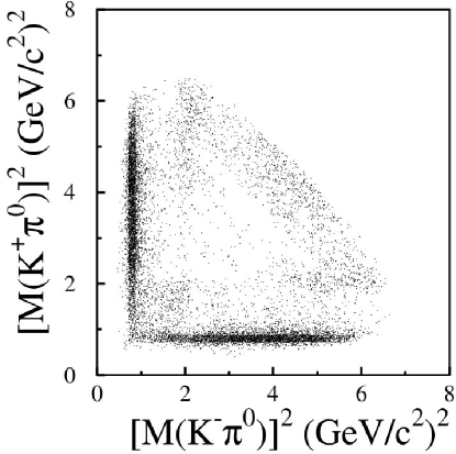
Figure 1: The $J/\psi\to K^{+}K^{-}\pi^{0}$ Dalitz plot distribution from the BESII Collaboration BES:2006 .

There is also a significant enhancement in the low $K^{+}K^{-}$ invariant mass region. In the BESII analysis this broad band was associated with a new isovector $P$-wave resonance, the $X(1570)$, decaying to $K^{+}K^{-}$ with the pole position at $(1576-409i)\mbox{ MeV}$ seen through a strong destructive interference with the $\rho(1700)$. There have been several theoretical attempts to explain this result Liu:2007 ; Li:2007 .

In this work we address the following questions. Can the broad enhancement in the low-mass $K{\bar{K}}$ channel be described by the $P$-wave $K{\bar{K}}$ amplitudes determined from phase shift analysis? And, more generally, can the Dalitz plot distribution of $K{\bar{K}}\pi$ events in the $J/\psi$ decay be described in terms of $K{\bar{K}}$ and $K\pi$ amplitudes reconstructed from phase shift analysis? To do so, we use, and further develop (by incorporating asymptotic energy dependence), the $P$-wave $\pi\pi$ and $K{\bar{K}}$ amplitudes initially constructed in Szczepaniak:2010re ; Guo:2010 . The amplitudes that we use have the correct analytical properties, satisfy two body unitarity and reproduce the known data on $\pi\pi$ scattering Hyams:1973 ; Protopopescu:1973 ; Estabrooks:1974 . In Guo:2010 we successfully used these amplitudes to describe the $J/\psi\to\pi^{+}\pi^{-}\pi^{0}$ Dalitz distribution. In particular we have found that, since the $\rho^{\prime\prime}(1700)$ is quite inelastic Hyams:1973 , destructive interference with the virtual $J/\psi\to K{\bar{K}}\pi\to 3\pi$ process is important in reducing the Dalitz plot intensity in the $\rho^{\prime\prime}$ resonance region. We will investigate if it is possible that a similar phenomena is in operation in the $K{\bar{K}}\pi$ final state and whether the virtual $J/\psi\to 3\pi\to K{\bar{K}}\pi$ decay may be responsible for the broad structure at low $K^{+}K^{-}$ invariant mass.

This paper is organized as follows. The partial wave decomposition of the decay $J/\psi\to K^{+}K^{-}\pi^{0}$ is given in Sec. II. In Sec. III, we discuss our $P$-wave amplitudes and compare with the BESII data of Fig. 1. Ideally, the set of partial waves that are developed here could be used in a full Dalitz plot analysis, but this requires a full knowledge of experimental acceptances and resolutions. In this work we simply compare, qualitatively, a sample of Dalitz plot distributions generated from our amplitudes with the BESII result of Fig. 1. We include more details on the amplitude construction in the appendices.

II Partial wave amplitudes in the $J/\psi\rightarrow K^{+}K^{-}\pi^{0}$ decay

Denoting the four momenta by $p_{\pm,0}$, $P$ for $K^{\pm}$, $\pi^{0}$ and $J/\psi$ respectively, the general expression for the $J/\psi\to K^{+}K^{-}\pi^{0}$ amplitude is given by,

$$\langle\pi^{0}K^{+}K^{-},out|J/\psi(\lambda),in\rangle=i(2\pi)^{4}\delta^{4}\left(\sum_{i=0,\pm}p_{i}-P\right)T_{\lambda}.$$ (1)

The Dalitz plot invariants are defined by $s_{ij}=(p_{i}+p_{j})^{2}$ with $i,j=\pm,0$ referring to $K^{\pm}$ and the $\pi^{0}$, respectively. The general expression for the helicity amplitude of $T_{\lambda}$ is given by

$$T_{\lambda}=\sum_{S,L}\sum_{\mu=\pm,0}N_{SL\mu}[D^{1*}_{\lambda,\mu}(r_{+-})d^{S}_{\mu,0}(\theta^{+}_{+-})F^{+-}_{SL}(s_{+-})+D^{1*}_{\lambda,\mu}(r_{+0})d^{S}_{\mu,0}(\theta^{+}_{+0})F^{+0}_{SL}(s_{+0})+D^{1*}_{\lambda,\mu}(r_{-0})d^{S}_{\mu,0}(\theta^{-}_{-0})F^{-0}_{SL}(s_{-0})]$$ (2)

where $N_{SL\mu}=\sqrt{3(2S+1)}\langle S\mu;L0|1\mu\rangle/4\pi$. Here $\lambda$ is the spin projection of the $J/\psi$ along the $e^{+}e^{-}$ beam axis, which together with $x$ and $y$ define a lab coordinate system, $S$ is the spin of a two particle subsystem (the isobar), and $L$ is the relative orbital angular momentum between the isobar and the spectator meson. The rotation $r_{ij}$ is given by three Euler angles, $r_{ij}=r_{ij}(\phi_{ij},\vartheta_{ij},\psi_{ij}^{i})$ which rotate the standard configuration in the $(ij)k$ coupling scheme, to the actual one. In the standard configuration of the $(ij)k$ coupling $J/\psi$ is at rest, particle $k$ has momentum along the negative $z$ axis, and particles $i$ and $j$ have momenta in the $xz$ plane with the particle $j$ moving in the positive $x$ direction. The azimuthal and polar angles, $\phi_{ij}$ and $\vartheta_{ij}$, are defined in the $J/\psi$ rest frame and refer to the actual direction of motion of the $(ij)$ pair. Finally, $\psi_{ij}^{i}$ and $\theta_{ij}^{i}$ are the azimuthal and the polar angle of the $i$-th particle in the $(ij)$, two-particle (isobar) rest frame.

The scalar form factors $F^{ij}_{SL}(s_{ij})$ describe the dynamics of the decay in the isobar model i.e. under the assumption that in a given isobar channel the form factors are functions of the sub-energy of that isobar only. In the $L-S$ basis, the parity of the $K^{+}K^{-}\pi^{0}$ state is given by $P=(-1)^{S+L+1}$ and under charge conjugation the two isobar channels, $|(K^{+}\pi^{0})K^{-}\rangle$ and $|(K^{-}\pi^{0})K^{+}\rangle$ are exchanged while the third isobar channel, $|(K^{+}K^{-})\pi^{0}\rangle$ is a charge conjugation eigenstate with the eigenvalue $(-1)^{S}$. Thus charge conjugation invariance implies that in Eq. (2) there are only two independent form factors which we define as,

$$F^{+-}_{SL}\equiv\frac{1-(-1)^{S}}{2}F^{K\bar{K}}_{SL},\ \ F^{+0}_{SL}=-F^{-0}_{SL}\equiv-F^{K\pi}_{SL}$$ (3)

and obtain,

$$T_{\lambda} = \sum_{S,L}\sum_{\mu=\pm 1,0}N^{\prime}_{SL\mu}[D^{1*}_{\lambda,\mu}(r_{+-})d^{S}_{\mu,0}(\theta^{+}_{+-})F^{+-}_{SL}(s_{+-})-D^{1*}_{\lambda,\mu}(r_{+0})d^{S}_{\mu,0}(\theta^{+}_{+0})F^{K\pi}_{SL}(s_{+0})+D^{1*}_{\lambda,\mu}(r_{-0})d^{S}_{\mu,0}(\theta^{-}_{-0})F^{K\pi}_{SL}(s_{-0})]$$

with $N^{\prime}_{SL\mu}\equiv N_{SL\mu}(1+(-1)^{S+L})/2$. The $\mu=0$ component vanishes due to parity conservation and we can further reduce the partial wave expansion to

$$T_{\lambda} = \sum_{S,L}N^{\prime}_{SL1}\{[D^{1*}_{\lambda,1}(r_{+-})+D^{1*}_{\lambda,-1}(r_{+-})]d^{S}_{1,0}(\theta^{+}_{+-})\frac{1-(-1)^{S}}{2}F^{K\bar{K}}_{SL}(s_{+-})$$ (5)

$$- [D^{1*}_{\lambda,1}(r_{+0})+D^{1*}_{\lambda,-1}(r_{+0})]d^{S}_{1,0}(\theta^{+}_{+0})F^{K\pi}_{SL}(s_{+0})+[D^{1*}_{\lambda,1}(r_{-0})+D^{1*}_{\lambda,-1}(r_{-0})]d^{S}_{1,0}(\theta^{-}_{-0})F^{K\pi}_{SL}(s_{-0})\}.$$

Finally, it is useful to rewrite the above amplitude in terms of a single set of angles describing orientation of the decay plane. Using the relation between Euler rotations,

$$r_{+-}=r_{-0}r(0,\chi_{+},0)=r_{+0}r^{-1}(0,0,\pi)r^{-1}(0,\chi_{-},0),$$ (6)

where $\chi_{+}(\chi_{-})$ is the angle between $K^{+}$ ($K^{-}$) and $\pi^{0}$ and in the $K^{+}K^{-}\pi^{0}$ rest frame enables to write $T$ in terms of $r_{+-}$ alone

$$T_{\lambda}=\sum_{S,L}N^{\prime}_{SL1}[D^{1*}_{\lambda,1}(r_{+-})+D^{1*}_{\lambda,-1}(r_{+-})][d^{S}_{1,0}(\theta^{+}_{+-})\frac{1-(-1)^{S}}{2}F^{K\bar{K}}_{SL}(s_{+-})+d^{S}_{1,0}(\theta^{+}_{+0})F^{K\pi}_{SL}(s_{+0})+d^{S}_{1,0}(\theta^{-}_{-0})F^{K\pi}_{SL}(s_{-0})].$$

The allowed quantum numbers in the $K^{+}K^{-}$ channel are $S^{PC}=1^{--}(\rho),3^{--}(\rho_{3}),\cdots$, and in the $K^{\pm}\pi^{0}$ channels, $S^{P}=1^{-}(K^{*}),2^{+}(K^{*}_{2}),3^{-}(K^{*}_{3}),\cdots$. In the following we will assume that the Dalitz distribution can be saturated with the lowest partial waves, i.e. $P$-wave in both $K^{+}K^{-}$ and $K^{\pm}\pi^{0}$ channels, and we test this hypothesis by studying the effect of the $D$-wave resonances in the $K\pi$ channels. Parity conservation implies $S=L$; therefore, in the following we will simply denote $F^{ij}_{SL}$ by $F_{L}^{ij}$. The (unnormalized) $J/\psi$ partial decay width with respect to one of the Dalitz invariants (e.g. $M_{K^{+}K^{-}}=\sqrt{s_{+-}}$) is obtained by integrating the square of the decay amplitude over the orientation of the decay plane and the other independent invariant,

$$\frac{d\Gamma}{d\sqrt{s_{+-}}}=N\sqrt{s_{+-}}\int^{s^{up}_{-0}(s_{+-})}_{s^{dn}_{-0}(s_{+-})}ds_{-0}|T|^{2},$$ (8)

and

$$|T|^{2}=|\sum_{S,L}N^{\prime}_{SL1}[d^{S}_{1,0}(\theta^{+}_{+-})\frac{1-(-1)^{S}}{2}F^{K\bar{K}}_{L}(s_{+-})$$ (9)

$$+ d^{S}_{1,0}(\theta^{+}_{+0})F^{K\pi}_{L}(s_{+0})+d^{S}_{1,0}(\theta^{-}_{-0})F^{K\pi}_{L}(s_{-0})]|^{2}.$$

The overall normalization ($N$) is adjusted to match the measured number of events. It is $|T|^{2}$ that determines the distribution of events in the Dalitz plot, (i.e. $|T|^{2}=const.$ would give a flat distribution). The integration limits, $s^{up/dn}_{-0}(s_{+-})$ are roots of the equation which define the boundary of the Dalitz plot,

$$s_{+-}s_{+0}s_{-0}-(s_{+0}+s_{-0})(m_{\pi}^{2}m_{K}^{2}+M^{2}m_{K}^{2})-s_{+-}(m_{K}^{4}+M^{2}m_{\pi}^{2})+2(m_{K}^{4}m_{\pi}^{2}+M^{2}m_{K}^{4}+2M^{2}m_{K}^{2}m_{\pi}^{2})=0.$$ (10)

Projections along $M_{K^{+}\pi}=\sqrt{s_{+0}}$ and $M_{K^{-}\pi}=\sqrt{s_{-0}}$ axis can be defined analogously.

In the following we discuss parameterizations of the form factors $F_{L}^{K\bar{K}}$ and $F_{L}^{K\pi}$ in terms of two-body amplitudes. Any parameters remaining in these parameterizations, which are related to the production process as opposed to final state interactions should be determined by fitting the Dalitz distributions. As discussed in Sec. I we do not fit the published Dalitz distribution, but instead show the predicted distributions for specific values of these parameters.

III Theoretical Model for Form Factors

Unitarity relates production form factors to two-body amplitudes. In  Szczepaniak:2010re ; Guo:2010 we constructed analytical representations for the isovector, $P$- wave, two-body, $\pi\pi$ and $K{\bar{K}}$ amplitudes. Here we further extend the analysis of  Guo:2010 by constraining the high energy behavior, and extend the approach to the $K\pi$ channel. We begin with a $K$-matrix, phenomenological parameterization of the known data (on the real axis) on phase shifts and elasticities. Even though the $K$-matrix offers an analytical representation for the amplitude, it often leads to spurious poles and zeros of the amplitude when extrapolated outside the physical region. Therefore we use the analytical representation for phase shifts and inelasticity via the $K$-matrix only in the data region and smoothly extrapolate to match with the asymptotic behavior of the partial waves at high energies. We then use the amplitudes constructed this way over the whole physical energy range as input into the Omnés-Muskhelishvili integral to construct the part of the scattering amplitude regular on the left side of the complex $s$-plane. With the $N(s)/D(s)$ representation, which is described below, we determine the amplitude over the entire $s$-plane. Finally we solve the unitarity relation for the form factors and write the $J/\psi$ decay amplitude in terms of the denominator functions $D(s)$ and production functions $c_{\alpha}(s)$. In the following we describe these steps in a little more detail. All details of the amplitude construction are given in the Appendix.

III.1 Amplitude Parameterization

In  Guo:2010 to describe the high energy limit of the isovector $P$-wave, the following hypothesis was made: the $S$ matrix is saturated by two channels, $\pi\pi$ and $K{\bar{K}}$ and the elastic channel phase shifts asymptotically approach a multiple of $\pi$ with elasticity $\eta$ approaching $1$. Even though $J/\psi$ decays probe only a limited energy range, and are quite insensitive to details of the asymptotic behavior we might as well use a different hypothesis that is better rooted in high energy phenomenology. It is known that at high energies, elastic cross sections slowly grow with energy almost approaching the Froissart bound. This implies that at impact parameter larger than the interaction region $O(1\mbox{ fm})$ there is no interaction while the low partial waves are suppressed as if scattering from a ”gray disk.” The low partial waves correspond to $L<<L_{0}(s)$ where $L_{0}(s)\sim\sqrt{s}/2\mbox{ fm}$ and while the interaction radius grows logarithmically with energy, the scattering of the low partial waves becomes logarithmically suppressed, i.e. $\eta_{L}\sim 1-O(1/\log s)$. In the language of Regge exchanges this picture corresponds to the Pomeron exchange at high energies. Furthermore, since asymptotically the number of inelastic channels grows rapidly, each individual inelastic amplitude, e.g $\pi\pi\to K{\bar{K}}$ is expected to fall off with energy, and is represented by exchange of non-vacuum quantum numbers, aka meson Regge trajectories. The hypothesis of two-channel dominance in the high energy limit is therefore not necessarily well justified and in the following we adopt the Regge picture of high energy scattering. Matching the $K$-matrix parameterization of the low energy data with Regge asymptotics, leads to amplitudes of the form (we drop the angular momentum label on the partial wave),

$$t_{\alpha,\beta}(s)=|t_{\alpha,\beta}(s)|e^{i\phi_{\alpha,\beta}(s)}=\left\{\begin{array}[]{c}t_{\alpha,\beta}^{Kmatrix}(s),s<s_{low}\\ t_{\alpha\beta}^{Regge}(s),s>s_{high}\end{array}\right.$$ (12)

with $t_{\alpha,\beta}^{Kmatrix}(s)$ and $t_{\alpha\beta}^{Regge}(s)$ determined from $K$-matrix fits to the low energy data and Regge fits to the high energy fixed $t$-data, respectively. Greek indices denote two body channels, i.e. $\alpha=(i,j)=\pi\pi,K\bar{K}$, etc. For energies between $s_{low}$ and $s_{high}$, we smoothly connect both real and imaginary parts of the $K$-matrix and Regge amplitudes. The denominator function in the $N/D$ parameterization

$$t_{\alpha\beta}(s)=\frac{N_{\alpha\beta}(s)}{D_{\alpha\beta}(s)}$$ (14)

is then obtained from the phase of the scattering amplitude using the Omnés-Muskhelishvili solution of the unitarity relation ($s_{th}\geq min(s_{\alpha},s_{\beta})$ where $s_{\alpha}$ is the $\alpha$-channel threshold)

$$\frac{\mbox{Im}D_{\alpha\beta}(s)}{D_{\alpha\beta}(s)}=-\sin\phi_{\alpha\beta}(s)e^{-2i\phi_{\alpha\beta}(s)}$$ (15)

and is given by

$$D_{\alpha\beta}(s)=e^{-\frac{s}{\pi}\int_{s_{th}}ds^{\prime}\frac{\phi_{\alpha\beta}(s^{\prime})}{s^{\prime}(s^{\prime}-s)}}$$ (16)

where we conveniently normalized $D_{\alpha\beta}(0)=1$. The numerator functions $N_{\alpha\beta}(s)$ are given by the largely unknown discontinuity of the amplitudes on the left hand cut. For the purpose of solving the unitarity relation for the $J/\psi$ decay form factors, which will be discussed below (cf. Eq. (18)), it is convenient to have $N_{\alpha\beta}(s)$’s for all intervening $\alpha,\beta$ channels having the same analytical form. This is certainly a simplifying approximation, nevertheless we have found that with a simple parameterization

$$N_{\alpha\beta}(s)=\frac{\lambda_{\alpha\beta}}{s+s_{L}}$$ (17)

and with the two-body amplitudes given by Eqs. (14),(16), it is indeed possible to obtain good fits to the two-body scattering data, i.e. phase shifts and elasticity.

Having constructed the two-body amplitudes, the next step is to relate them to the production form factors. This is done through the unitarity relations which relate the imaginary part of the form factors to the two-body amplitudes,

$$\mbox{Im}\hat{F}^{\alpha}_{L}(s)=\sum_{\beta}t^{*}_{\alpha,\beta}(s)\rho^{\beta}(s)\hat{F}^{\beta}_{L}(s)$$ (18)

with ${}_{\alpha\beta}t$ representing the elastic $L$-partial wave scattering amplitude between two-body channels $\alpha=(ij)$ and $\beta=(i^{\prime}j^{\prime})$. $\hat{F}$ is the reduced form factor (with the barrier factor removed),

$$F_{L}^{ij}(s)=q^{L}_{ij}(s)p^{L}_{k}(s)\hat{F}^{ij}_{L}(s),$$ (19)

with $q_{ij}(s)$ being the relative momentum between mesons $i$ and $j$,

$$q_{ij}(s)=\sqrt{\frac{[s-(m_{i}+m_{j})^{2}][s-(m_{i}-m_{j})^{2}]}{4s}}$$ (20)

and

$$p_{k}(s)=\sqrt{\frac{[s-(M+m_{k})^{2}][s-(M-m_{k})^{2}]}{4M^{2}}},$$ (21)

with $M$ being the $J/\psi$ mass, the relative momentum between the $(ij)$ pair and the spectator meson $k$. $\rho_{\alpha}(s)=2q_{ij}/\sqrt{s}$ describes the two-particle phase space. It is straightforward to show that if the scattering amplitude is dominated by a single resonance below inelastic threshold ($\rho=\rho^{\alpha}$, $\rho^{\beta}=0$ for $\beta\neq\alpha$) the solution of the unitarity condition for $\hat{F}$ is

$$\hat{F}^{\alpha}_{L}(s)=c(s)BW^{L}_{R}(s)=\frac{c(s)}{m_{R}^{2}-s-im_{R}\Gamma_{L}(s)},$$ (22)

where $BW^{L}_{R}(s)$ is the Breit-Wigner amplitude (with an energy dependent width $\Gamma_{L}(s)$) and $c(s)$ is a real polynomial in $s$. In the general multiple-channel case, with the two-body amplitudes all parameterized by the same numerator function, as in Eq. (17) the solution to Eq. (18) is given by Pham:1976yi ,

$$\hat{F}^{\alpha}(s)=\sum_{\beta}\frac{c_{\beta}(s)}{D^{\alpha\beta}(s)}$$ (23)

with $c_{\beta}(s)$ being analytic functions in the right hand plane and $\mbox{Im}c_{\alpha}(s)=0$ for $s>0$.

III.2 Results

As discussed in Sec. I the original BESII analysis was based on the isobar, resonance parameterization of all three two-body channels. In the absence of a known isovector $P$-wave $K{\bar{K}}$ resonance to describe the low mass $K{\bar{K}}$ enhancement, it was necessary to introduce a new resonance, the $X(1570)$. The $\pi\pi$ phase isovector $P$-wave shift data, however, points to significant inelasticity above $1.6\mbox{ GeV}$, which following Hyams:1973 we have attributed to the $K{\bar{K}}$ channel. The effect of the coupled $\pi\pi$ and $K{\bar{K}}$ channels on the $K^{+}K^{-}\pi^{0}$ mass distribution which follows from Eq. (23) is shown in Fig. 2.

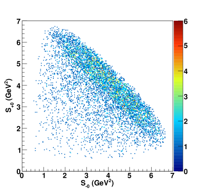
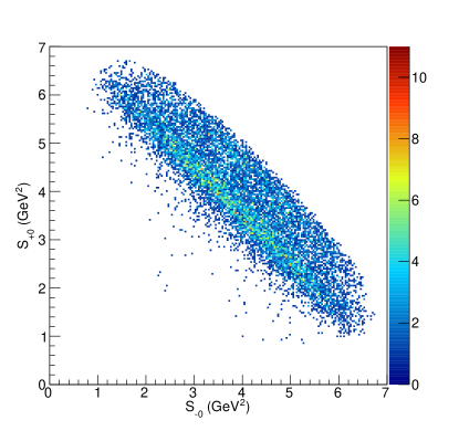
Figure 2: Dalitz plot distribution obtained using, in Eq. (23), a single two-body $K\bar{K}\to K\bar{K}$ amplitude (top) and a single two-body $\pi\pi\to K\bar{K}$ amplitude (bottom) (i.e. with $c_{K\bar{K}}=1$ ($c_{\pi\pi}=1$) for the top (bottom) and $c_{\alpha}(s)=0$ for all other waves).

In Fig. 3 we show the Dalitz distribution obtained using the single $K\pi$ channel amplitude (details discussed in the Appendix). Besides the $K^{*}(892)$ peaks, bands at $M_{K\pi}=1.75\mbox{ GeV}$ are clearly visible in both $K^{+}\pi^{0}$ and $K^{-}\pi^{0}$ mass projections. These are due to the $K^{*}(1680)$ resonance clearly seen in the $K\pi$ phase shift analysis Aston:1988 ; Mercer:1971 ; Estabrooks:1978 but apparently not so in the $K\pi$ production from the $J/\psi$ decay (cf. Fig. 1). This clear discrepancy indicates that it is not sufficient to use a single channel $K\pi$ amplitude in the parameterization of the corresponding form factor in the $J/\psi$ decay. As discussed in the Appendix the $K\pi$ amplitude is indeed inelastic above $M_{K\pi}\sim 1.5\mbox{ GeV}$ with a possibility of a large coupling to the $K^{*}(892)\pi$ channel.

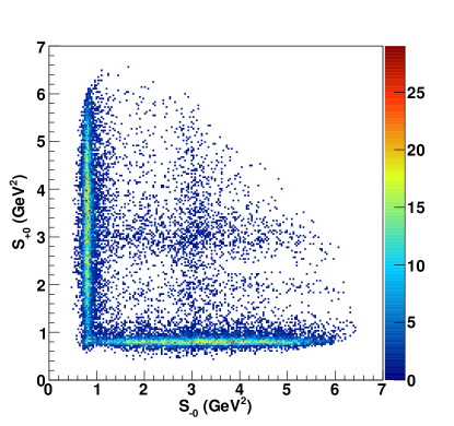
Figure 3: As in Fig. 2 but with a single two-body, $K\pi\to K\pi$ amplitude.

Finally, in Fig. 4 we show the Dalitz distribution obtained with a combination of three amplitudes, $K{\bar{K}}\to K{\bar{K}}$, $\pi\pi\to K{\bar{K}}$ and $K\pi\to K\pi$ with relative production coefficients, $c_{\alpha}(s)$ chosen to best match the observed distribution in Fig. (1). While the low mass $K\bar{K}$ region seems to be fairly well described, the resonance structures in he $K\pi$ channel do not match between the elastic $t_{K\pi\to K\pi}$ and $J/\psi$ decay amplitude. The $\pi\pi\to K\bar{K}$ and $K\bar{K}\to K\bar{K}$ amplitudes behave rather smoothly in the region corresponding to the $K\pi$ resonances and do not give enough strength to reducing the peak from the second $K^{*}$ resonance region. Thus we anticipate that the discrepancy is due to inelasticities in the $K\pi$ channel itself. Since we are only comparing Dalitz distributions as opposed to fitting data, we do not attempt to further improve the comparison. It is worth noting that the $K^{*}(1410)$ listed in the PDG is indeed quite inelastic with only a $6.6\%$ branching to $K\pi$.

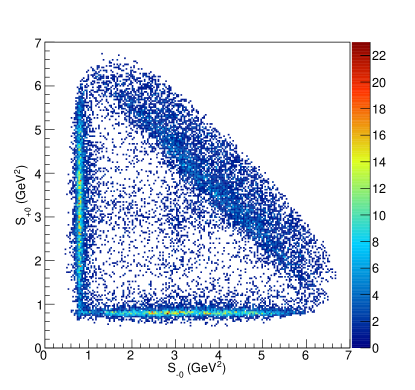
Figure 4: As in Fig. 2 but with three amplitudes, $K{\bar{K}}\to K{\bar{K}}$, $\pi\pi\to K{\bar{K}}$ and $K\pi\to K\pi$ with relative production coefficients satisfying $c_{K\pi}(s):c_{K\bar{K}}(s):c_{\pi\pi}(s)=1:0.3:-0.7$.

IV Discussion and conclusion

Based on unitarity and analyticity we have constructed a set of analytical two-body amplitudes, which implement the known phase shift data. These extend our previous work in coupled channel $P$-wave $\pi\pi$ and $K\bar{K}$ systems and the $J/\psi\to 3\pi$ decay Guo:2010 . The two-body amplitudes are only an approximation to the three-body decay, nevertheless they provide a useful starting point and should match below inelastic thresholds. We compared the analysis of the $J/\psi$ decay with these amplitudes to the original analysis of the BESII collaboration, which was based on the isobar model with coherent Breit-Wigner resonances. The isobar model with the known, low mass resonances only and without inelasticities cannot faithfully produce the broad structure of low $K^{+}K^{-}$ invariant mass, which is why in the BESII analysis an additional $P$-wave resonance $X(1576)$ coupled to $K^{+}K^{-}$ was introduced. Our preliminary study indicates that the $K\bar{K}$ low-mass region may be described by the inelasticity in the $\pi\pi\to\pi\pi$ wave if attributed to the coupling between $\pi\pi$ and $K\bar{K}$ channels. A single $K\pi\to K\pi$ amplitude is strongly affected by the second vector $K^{*}(1680)$ resonance as observed in $K\pi$ phase shift analysis. However, in $J/\psi$ decay this resonance seems to be suppressed. It is worth noting that a similar suppression of the first excited isovector-vector resonance is also observed in the $3\pi$ decay of $J/\psi$ Guo:2010 .

V Acknowledgments

The authors would like to thank Mikhail Gorchtein for helpful discussion. This work was supported in part by the US Department of Energy grant under contract DE-FG0287ER40365, National Science Foundation PIF grant number 0653405.

Appendix A Analytical model for the $P$-wave isovector $\pi\pi\to\pi\pi$, $\pi\pi\to K\bar{K}$ and $K{\bar{K}}\to K{\bar{K}}$ amplitudes

A.1 $K$-matrix parameterization, ($s<s_{low}$)

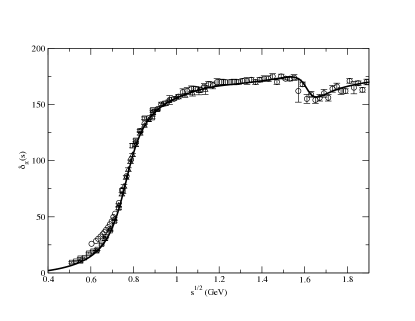
Figure 5: Phase shift of the $P$-wave $\pi\pi$ amplitude. Data is taken from Hyams:1973 (circles) ,Protopopescu:1973 (triangles) , and Estabrooks:1974 (squares). The solid line is the result of the fit to $\delta_{\pi}$ and $\eta$ with the analytical $K$-matrix representation described in the text.

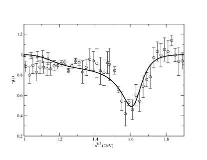
Figure 6: Same as in Fig. 5 for the inelasticity $\eta$

We use a two channel $K$-matrix Guo:2010 to fit the data on $\pi\pi\to\pi\pi$ $P$-wave phase shift and elasticity $\eta$ from Hyams:1973 ; Protopopescu:1973 ; Estabrooks:1974 (Fig. 5,6). With the $S$-matrix saturated by two channels, the model makes a prediction for the phase shift in the $K{\bar{K}}\to K{\bar{K}}$ channel. In this section $\alpha,\beta=\pi,K$ correspond to the two body channels $\pi\pi$ and $K{\bar{K}}$, respectively. The 2-channel $K$-matrix representation is given by

$$[\hat{t}^{-1}(s)]_{\alpha\beta}=[K^{-1}(s)]_{\alpha\beta}+\delta_{\alpha\beta}(s-s_{\alpha})I_{\alpha}(s),$$ (24)

where

$$I_{\alpha}(s)=I_{\alpha}(0)-\frac{s}{\pi}\int_{s_{\alpha}}^{\infty}ds^{\prime}\sqrt{1-\frac{s_{\alpha}}{s^{\prime}}}\frac{1}{(s^{\prime}-s)s^{\prime}}.$$ (25)

A convenient choice for the subtraction constant, $I_{\alpha}(0)$, is to take $\mbox{Re}I_{\alpha}(M^{2}_{\rho})=0$ so that one of the poles of $K_{\pi\pi}$ corresponds to the Breit-Wigner mass squared, $M^{2}_{\rho}=(0.77\mbox{ GeV})^{2}$, of the $\rho$ meson. Using the general two-pole parameterization of the $K$ matrix,

$$K_{\pi\pi}=\frac{\alpha_{\pi}^{2}}{M_{\rho}^{2}-s}+\frac{\beta_{\pi}^{2}}{s_{2}-s}+\gamma_{\pi\pi},\;K_{KK}=\frac{\beta^{2}_{K}}{s_{2}-s}+\gamma_{KK}$$

$$K_{\pi K}=K_{K\pi}=\frac{\beta_{\pi}\beta_{K}}{s_{2}-s}+\gamma_{\pi K},$$ (26)

where $\alpha_{\pi}^{2}=\Gamma_{\rho}M^{2}_{\rho}/(M_{\rho}^{2}-s_{\pi})^{3/2}$ and fitting the $P$-wave $\pi\pi$ phase shift, $\delta_{\pi}$, and the elasticity, $\eta$, we obtain $\Gamma_{\rho}=0.140\mbox{ GeV}$, and

$$\sqrt{s_{2}}=1.4708\mbox{ GeV},\ \ \ \ \beta_{\pi}=0.199,\ \ \ \ \beta_{K}=0.899,$$

$$\gamma_{\pi\pi}=5.62\times 10^{-2},\ \ \ \ \ \gamma_{\pi K}=0.104,\ \ \ \ \ \gamma_{KK}=1.525,$$

with the $\gamma$’s in units of $\mbox{ GeV}^{-2}$. The comparison of the phase shift and the inelasticity obtained with this parameterization with the data is shown in Fig. 5,6. To illustrate unphysical features of the $K$-matrix parameterization we rewrite Eq. (24) using the standard $N/D$ representation for $\hat{t}_{\alpha\beta}=t_{\alpha\beta}/(4q_{\alpha}q_{\beta})$. With the normalization $D_{\alpha\beta}(0)=1$ we obtain,

$$N_{\pi\pi}(s)=\lambda_{\pi\pi}\frac{s-z_{\pi\pi}}{(s-s_{L,1})(s-s_{L,2})},\;D_{\pi\pi}(s)=\exp\left(-\frac{s}{\pi}\int_{s_{\pi}}ds^{\prime}\frac{\phi_{\pi\pi}(s^{\prime})}{s^{\prime}(s^{\prime}-s)}\right),$$

$$N_{\pi K}(s)=\frac{\lambda_{\pi K}}{(s-s_{L,1})(s-s_{L,2})},\;D_{\pi K}(s)=\frac{s_{1,\pi K}s_{2,\pi K}}{(s-s_{1,\pi K})(s-s_{2,\pi K})}\exp\left(-\frac{s}{\pi}\int_{s_{\pi}}ds^{\prime}\frac{\phi_{\pi K}(s^{\prime})}{s^{\prime}(s^{\prime}-s)}\right),$$

$$N_{KK}(s)=\lambda_{KK}\frac{s-z_{KK}}{(s-s_{L,1})(s-s_{L,2})},\;D_{KK}(s)=\exp\left(-\frac{s}{\pi}\int_{s_{\pi}}ds^{\prime}\frac{\phi_{KK}(s^{\prime})}{s^{\prime}(s^{\prime}-s)}\right),$$ (28)

with $\lambda_{\pi\pi}=5.649$, $\lambda_{KK}=2.271$ and $\lambda_{\pi K}=3.048\mbox{ GeV}^{2}$. In this $K$-matrix model, the left hand cut of $N$ is reduced to two poles at $s_{L,1}=-13.87\mbox{GeV}^{2}$ and $s_{L,2}=-0.787\mbox{ GeV}^{2}$, respectively. There are also first order zeros in $N_{\alpha\beta}$ at $z_{\pi\pi}=-0.867\mbox{ GeV}^{2}$ and $z_{KK}=-13.78\mbox{GeV}^{2}$. Above the $K{\bar{K}}$ threshold the phase of the inelastic amplitude $\phi_{\pi K}$ is given by $\phi_{\pi K}=\delta_{\pi}+\delta_{K}$. From the $K$ matrix we find that, asymptotically, $\phi_{\pi K}(\infty)=2\pi$, which corresponds to two CDD poles: one at the $\rho$ mass, $s_{1,\pi K}=M_{\rho}^{2}$, and the other at $s_{2,\pi K}=s_{2}+\beta_{\pi}\beta_{K}/\gamma_{\pi K}=3.884\mbox{ GeV}^{2}$. Thus, while the $K$ matrix parameterization faithfully reproduces the $\pi\pi$ phase shift and elasticity in the whole available energy range, from $\pi\pi$ threshold up to $1.9\mbox{ GeV}$, extrapolation beyond this range is problematic. The rapid decrease of $\phi_{\pi\pi}$ around $s\sim 6\mbox{ GeV}^{2}$ seems unphysical. In the $\pi\pi\to K{\bar{K}}$ channel, the two CDD poles at $m_{\rho}^{2}$ and $s_{2}+\beta_{\pi}\beta_{K}/\gamma_{\pi K}$ are clearly an artifact of the pole parameterization of the $K$-matrix. A CDD pole in the inelastic channel above threshold (cf. the pole at $s_{2,\pi K}=3.884\mbox{ GeV}^{2}$) leads to a discontinuity in a phase shift and is unphysical. It also implies vanishing inelasticity, $\eta=1$ at this energy. A pole between $\pi\pi$ and $K{\bar{K}}$ thresholds is admissible, e.g. the pole at $s_{1,\pi K}=m_{\rho}^{2}$, but its strict overlap with the $\rho$ mass is also an artifact of the parameterization. Since the phase space available in $J/\psi$ decay extends up to $s_{\pi\pi}\sim 9\mbox{GeV}^{2}$ we need to remove these unphysical features of the $K$-matrix amplitude. As discussed in Sec. III we do this by using the $K$-matrix amplitudes below $s_{low}$ and above $s_{high}$ we will use Regge parameterization.

A.2 Regge parameterization ($s>s_{high}$)

Regge analysis of $\pi\pi\rightarrow\pi\pi$ scattering has been studied recently in pelaez:2004 ; Ananthanarayan:2001 ; pelaez:2005 and here we use the results of  pelaez:2005 . Parameters in Regge amplitudes were constrained by analyzing $NN$, $\pi N$ and $\pi\pi$ scattering data. For completeness we give the relevant formulas below.

• $\pi\pi\to\pi\pi$

Regge parameterization involves the Regge poles corresponding to $t$-channel exchange of the Pomeron($P$), the $P^{\prime}$ (associated with the $f_{2}(1270)$ trajectory) and the $\rho$. The $t$-channel isospin amplitudes are given by

$$F^{(I_{t}=0)}_{\pi\pi}(t,s,u)$$

$$= -\frac{1+e^{-i\pi\alpha_{P}(t)}}{\sin\pi\alpha_{P}(t)}P(s,t)-\frac{1+e^{-i\pi\alpha_{P^{\prime}}(t)}}{\sin\pi\alpha_{P^{\prime}}(t)}P^{\prime}(s,t),$$

$$F^{(I_{t}=1)}_{\pi\pi}(t,s,u)$$

$$= \frac{1-e^{-i\pi\alpha_{\rho}(t)}}{\sin\pi\alpha_{\rho}(t)}\beta_{\rho}\frac{1+\alpha_{\rho}(t)}{1+\alpha_{\rho}(0)}[1+d_{\rho}t]e^{bt}(s/\hat{s})^{\alpha_{\rho}(t)},$$

$$\mbox{Im}F^{(I_{t}=2)}_{\pi\pi}(t,s,u)=\beta_{2}e^{bt}(s/\hat{s})^{\alpha_{\rho}(t)+\alpha_{\rho}(0)-1}.$$

where ($\hat{s}=1\mbox{ GeV}$)

$$P(s,t) = \beta_{P}\alpha_{P}(t)\frac{1+\alpha_{P}(t)}{2}e^{bt}(s/\hat{s})^{\alpha_{P}(t)},$$ (32)

$$P^{\prime}(s,t) = \beta_{P^{\prime}}\frac{\alpha_{P^{\prime}}(t)[1+\alpha_{P^{\prime}}(t)]}{\alpha_{P^{\prime}}(0)[1+\alpha_{P^{\prime}}(0)]}e^{bt}(s/\hat{s})^{\alpha_{P^{\prime}}(t)},\ \ \ \ \$$ (33)

and the trajectories are given by

$$\alpha_{P}(t)=\alpha_{P}(0)+t\alpha^{\prime}_{P},$$

$$\alpha_{P^{\prime}}(t)=\alpha_{\rho}(t)=\alpha_{\rho}(0)+t\alpha^{\prime}_{\rho}+\frac{1}{2}t^{2}\alpha^{\prime\prime}_{\rho}.$$ (34)

Numerical values of all parameters are given in Eqs. (B5), (B6) of pelaez:2005 . The $s$-channel isospin, partial wave amplitudes are normalized according to

$$F^{(I_{s})}_{\alpha,\beta}(s,t,u)=(\sqrt{2})^{\sigma}\frac{4}{\pi}\sum_{L}(2L+1)t^{(LI_{s})}_{\alpha,\beta}(s)P_{L}(\cos\theta),$$

where $(\sqrt{2})^{\sigma}$ is the identical particle symmetry factor: $\sigma=2$ for $\pi\pi\leftrightarrow\pi\pi$, $\sigma=1$ for $\pi\pi\leftrightarrow K\bar{K}$ and $\sigma=0$ for $K\bar{K}\leftrightarrow K\bar{K}$. The $s$-channel amplitudes with $I_{s}=0,2$ are symmetric under $t\leftrightarrow u$ exchange, and the $I_{s}=1$ amplitude is antisymmetric and $s\leftrightarrow t$ crossing leads to the following relation between the $s$ and the $t$-channel isospin amplitudes,

$$F^{(I_{s}=1)}_{\pi\pi}(s,t,u) = \frac{1}{3}F^{(I_{t}=0)}_{\pi\pi}(t,s,u)+\frac{1}{2}F^{(I_{t}=1)}_{\pi\pi}(t,s,u)$$ (36)

$$- \frac{5}{6}F^{(I_{t}=2)}_{\pi\pi}(t,s,u)-(t\rightarrow u).$$

The $(t\leftrightarrow u)$ exchange brings in the u-channel Regge poles (these were ignored in pelaez:2005 where only the forward $t=0$ limit was considered). Finally, projecting out the $P$-wave amplitude yields,

$$t^{Regge}_{\pi\pi}(s)=\frac{\pi}{16}\int_{-1}^{1}(d\cos\theta)\cos\theta$$ (37)

$$\times [\frac{1}{3}F^{(I_{t}=0)}_{\pi\pi}(t,s,u)+\frac{1}{2}F^{(I_{t}=1)}_{\pi\pi}(t,s,u)$$

$$- \frac{5}{6}F^{(I_{t}=2)}_{\pi\pi}(t,s,u)-(t\rightarrow u)].$$

The angular integration is done numerically. The leading asymptotic behavior due to Pomeron exchange can be calculated analytically and is given by,

$$t^{Regge}_{\pi\pi}(s)\simeq i\frac{\pi}{16}\frac{1}{3}\int_{-1}^{1}(d\cos\theta)\cos\theta[P(s,t)-P(s,u)]$$ (38)

$$\simeq i\frac{\pi}{24}\beta_{P}\frac{-3\alpha^{\prime}_{P}+2(b+\alpha^{\prime}_{P}\ln s)}{(b+\alpha^{\prime}_{P}\ln s)^{2}}s^{\alpha_{P}(0)-1}.$$

To combine the $K$-matrix ($s<s_{low}$) with the Regge projected ($s>s_{high}$) amplitudes into the full $P$-wave $\pi\pi\to\pi\pi$ amplitude,

$$t_{\pi\pi}(s)=\left\{\begin{array}[]{c}t_{\pi\pi}^{Kmatrix}(s),s<s_{low}\\ t_{\pi\pi}^{Regge}(s),s>s_{high}\end{array}\right.,$$ (41)

we choose $\sqrt{s_{low}}=2.20\mbox{ GeV}$ and $\sqrt{s_{high}}=2.56\mbox{ GeV}$, and use a simple analytical formula to smoothly join the two amplitudes between $s_{low}$ and $s_{high}$. The result is shown in Fig. 7.

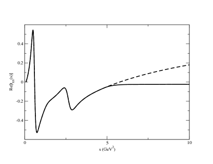
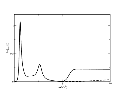
Figure 7: Real (top) and imaginary (bottom) parts of the isovector, $P$-weave amplitude, $t_{\pi\pi}(s)$ (solid lines). Dashed line is the result of the $K$-matrix parameterization.

• $\pi\pi\to K{\bar{K}}$

Asymptotically the $t$-channel amplitude it is dominated by the $K^{*}$ trajectory,

$$F^{(I_{t}=\frac{1}{2})}_{\pi K}(t,s,u)$$

$$= \frac{1-e^{-i\pi\alpha_{K^{*}}(t)}}{\sin\pi\alpha_{K^{*}}(t)}\beta_{K^{*}}\frac{2\alpha_{K^{*}}(t)+1}{2\alpha_{K^{*}}(0)+1}e^{bt}(\alpha^{\prime}_{K^{*}}s)^{\alpha_{K^{*}}(t)}.$$

Following Ananthanarayan:2002 we use $b=2.4$ $GeV^{-2}$, and $\alpha_{K^{*}}(t)=0.352+\alpha^{\prime}_{K^{*}}t$ with $\alpha^{\prime}_{K^{*}}=0.882GeV^{-2}$. The $s$-channel $I_{s}=1/2$ amplitude is antisymmetric under $t\leftrightarrow u$ exchange,

$$F^{(I_{s}=1)}_{\pi K}(s,t,u)=-F^{(I_{s}=1)}_{\pi K}(s,u,t).$$ (43)

and from $s\leftrightarrow t$ crossing we obtain,

$$F^{(I_{s}=1)}_{\pi K}(s,t,u)$$

$$= \frac{2}{3}F^{(I_{t}=\frac{1}{2})}_{\pi K}(t,s,u)-\frac{2}{3}F^{(I_{t}=\frac{3}{2})}_{\pi K}(t,s,u)-(t\rightarrow u).$$

In terms of $F^{(I_{s}=1)}_{\pi K}(s,t,u)$ the properly normalized $P$-wave in $\pi\pi\to K{\bar{K}}$ is finally given by

$$t^{Regge}_{\pi K}(s)=\frac{\pi}{8\sqrt{2}}\int_{-1}^{1}(d\cos\theta)\cos\theta$$ (45)

$$\times \left[\frac{2}{3}F^{(I_{t}=\frac{1}{2})}_{\pi K}(t,s,u)-(t\rightarrow u)\right].$$

We can fix $\beta_{K^{*}}$ by matching our formula in Eq. (A.2) to Eq. (81) in Ananthanarayan:2002 in the limit of $t\rightarrow 0$ (forward direction). Taking into account differences in normalization employed here and used in Ananthanarayan:2002 , we find

$$\mbox{Im}F^{(I_{t}=\frac{1}{2})}_{\pi K}(t,s,u)|_{s\rightarrow\infty,t\rightarrow 0}$$

$$= \beta_{K^{*}}(\alpha^{\prime}_{K^{*}}s)^{\alpha_{K^{*}}(0)}=\frac{3}{4\pi}\frac{\lambda}{\Gamma[\alpha_{K^{*}}(0)]}(\alpha^{\prime}_{K^{*}}s)^{\alpha_{K^{*}}(0)}$$

with $\lambda=1.82$ taken from Ananthanarayan:2002 and

$$\beta_{K^{*}}=\frac{3}{4\pi}\frac{\lambda}{\Gamma[\alpha_{K^{*}}(0)]}=0.172.$$ (47)

Asymptotically, $t^{Regge}_{\pi K}(s)$ approaches

$$t^{Regge}_{\pi K}(s) \simeq \frac{1-e^{-i\pi\alpha_{K^{*}}(0)}}{\sin\pi\alpha_{K^{*}}(0)}\beta_{K^{*}}\frac{\pi}{8\sqrt{2}}\frac{2}{3}\int_{-1}^{1}(d\cos\theta)\cos\theta[\frac{2\alpha_{K^{*}}(t)+1}{2\alpha_{K^{*}}(0)+1}e^{bt}(\alpha^{\prime}_{K^{*}}s)^{\alpha_{K^{*}}(t)}-(t\rightarrow u)]$$

$$\simeq \frac{1-e^{-i\pi\alpha_{K^{*}}(0)}}{\sin\pi\alpha_{K^{*}}(0)}\frac{\pi}{3\sqrt{2}}\frac{\beta_{K^{*}}\alpha^{\prime}_{K^{*}}}{2\alpha_{K^{*}}(0)+1}\frac{(1+2\alpha_{K^{*}}(0))[b+\alpha^{\prime}_{K^{*}}\ln(\alpha^{\prime}_{K^{*}}s)]-2\alpha^{\prime}_{K^{*}}}{[b+\alpha^{\prime}_{K^{*}}\ln(\alpha^{\prime}_{K^{*}}s)]^{2}}(\alpha^{\prime}_{K^{*}}s)^{\alpha_{K^{*}}(0)-1}.$$

]The complete amplitude is given by,

$$t_{\pi K}(s)=\left\{\begin{array}[]{c}t_{\pi K}^{Kmatrix}(s),s<s_{low}\\ t_{\pi K}^{Regge}(s),s>s_{high}\end{array}\right.\ \ \ \ \ \ \ \$$ (51)

where we choose $\sqrt{s_{low}}=2.5$GeV and $\sqrt{s_{high}}=3$GeV and it is shown in Fig. 8.

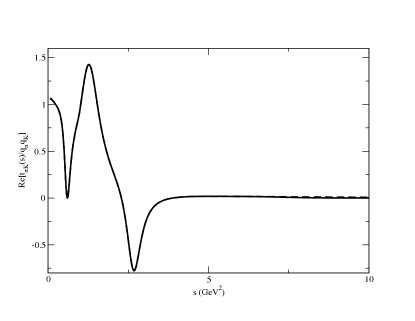
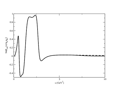
Figure 8: Real (top) and imaginary (bottom) parts of the isovector, $P$-wave amplitude, $t_{\pi K}(s)/(q_{\pi}q_{K})$ (solid lines). The dashed line is the result of the $K$-matrix parameterization.

• $K\bar{K}\to K\bar{K}$

Asymptotically we only retain the Pomeron exchange,

$$F^{(I_{t}=0)}_{K\bar{K}}(t,s,u)$$

$$= -\frac{1+e^{-i\pi\alpha_{P}(t)}}{\sin\pi\alpha_{P}(t)}\beta^{K\bar{K}}_{P}\alpha_{P}(t)\frac{1+\alpha_{P}(t)}{2}e^{bt}(s/\hat{s})^{\alpha_{P}(t)}.$$

with $\alpha_{P}(t)=\alpha_{P}(0)+t\alpha^{\prime}_{P}$ and all other parameters, except $\beta^{K\bar{K}}_{P}$ taken from pelaez:2005 ; pelaez:2004 , while for the Pomeron coupling to $K{\bar{K}}$ we use relation $\beta^{K\bar{K}}_{P}=(\frac{f^{(P)}_{K}}{f^{(P)}_{\pi}})^{2}(f_{\pi}^{(P)})^{2}=1.15$, where the values of $\frac{f^{(P)}_{K}}{f^{(P)}_{\pi}}$ and $\beta_{P}=(f^{(P)}_{\pi})^{2}$ are taken from pelaez:2005 ; pelaez:2004 . From $s\leftrightarrow t$ crossing,

$$F^{(I_{s}=1)}_{K\bar{K}}(s,t,u)=\frac{1}{2}F^{(I_{t}=0)}_{K\bar{K}}(t,s,u)-\frac{1}{2}F^{(I_{t}=1)}_{K\bar{K}}(t,s,u).$$

For the Pomeron contribution to the $s$-channel $P$-wave we thus find

$$t^{Regge}_{K\bar{K}}(s)=\frac{\pi}{8}\int_{-1}^{1}(d\cos\theta)\cos\theta\frac{1}{2}F^{I_{t}=0}_{K\bar{K}}(t,s,u).$$ (54)

Asymptotically, $t^{Regge}_{K\bar{K}}(s)$ is given by

$$t^{Regge}_{K\bar{K}}(s)$$ (55)

$$\simeq i\frac{\pi}{16}\beta^{K\bar{K}}_{P}\int_{-1}^{1}(d\cos\theta)\cos\theta\alpha_{P}(t)\frac{1+\alpha_{P}(t)}{2}e^{bt}s^{\alpha_{P}(t)}$$

$$\simeq i\frac{\pi}{16}\beta^{K\bar{K}}_{P}\frac{-3\alpha^{\prime}_{P}+2(b+\alpha^{\prime}_{P}\ln s)}{(b+\alpha^{\prime}_{P}\ln s)^{2}}s^{\alpha_{P}(0)-1}.$$

In the full amplitude,

$$t_{K\bar{K}}(s)=\left\{\begin{array}[]{c}t_{K\bar{K}}^{Kmatrix}(s),s<s_{low}\\ t_{K\bar{K}}^{Regge}(s),s>s_{high}\end{array}\right..$$ (58)

we take $\sqrt{s_{low}}=1.62$ GeV and $\sqrt{s_{high}}=3$ GeV for real parts of amplitudes, and $\sqrt{s_{low}}=1.64$ GeV and $\sqrt{s_{high}}=1.8$ GeV for imaginary parts of amplitudes. The different choice for the real and imaginary parts allows for a smoother connection with the Regge asymptotics. The phase of $t_{K\bar{K}}^{Regge}(s)$ asymptotically approaches $\pi/2$ but the phase of $t_{K\bar{K}}^{Kmatrix}(s)$ has a sharp drop above $1.65$ GeV (see right plot in Fig. 10). Therefore, choosing $\sqrt{s_{low}}\sim 1.64$ GeV allows for a continuous match between the phases of $t_{K\bar{K}}(s)$, as show in Fig. 9.

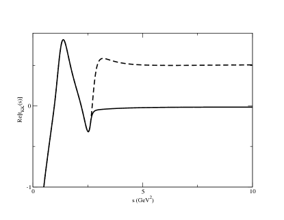
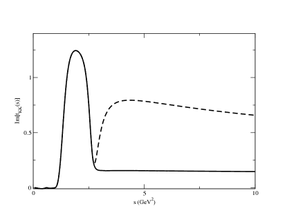
Figure 9: Real (top) and imaginary (bottom) parts of the isovector, $P$-wave amplitude, $t_{K\bar{K}}(s)$ (solid lines). The dashed line is the result of the $K$-matrix parameterization.

A.3 Phases of amplitudes and $D$ functions

From Regge parameterizations we find the following asymptotic behavior for the phases $\phi_{\alpha\beta}(s)$ of the complete amplitudes,

$$\phi_{\pi\pi}\rightarrow\arctan[-\frac{\sin\pi\alpha_{P}(0)}{1+\cos\pi\alpha_{P}(0)}]=\frac{\pi}{2},$$ (59)

$$\phi_{\pi K}\rightarrow 2\pi+\arctan[\frac{\sin\pi\alpha_{K^{*}}(0)}{1-\cos\pi\alpha_{K^{*}}(0)}]\simeq 2\pi+\frac{\pi}{3},\ \ \ \ \ \ \ \$$ (60)

$$\phi_{K\bar{K}}\rightarrow\arctan[-\frac{\sin\pi\alpha_{P}(0)}{1+\cos\pi\alpha_{P}(0)}]=\frac{\pi}{2}.$$ (61)

These are shown in Fig. 10.

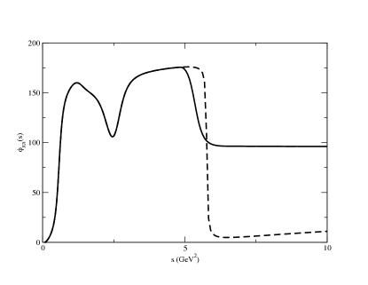
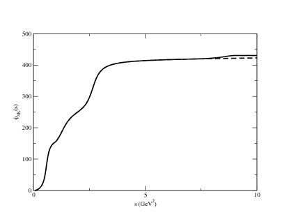
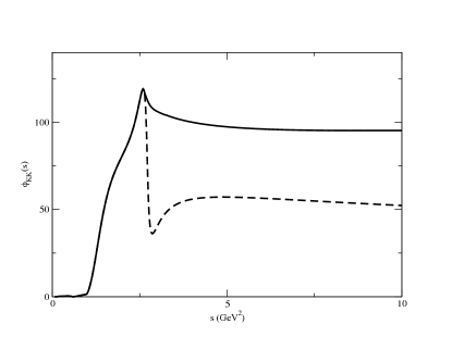
Figure 10: Phase of the $\pi\pi$ (top), $\pi K$ (middle) and $K\bar{K}$ (bottom) $P$-wave amplitude. The dashed line is the result of the $K$-matrix parameterization from Eq. (28).

For the $D$ functions test lead to the following asymptotic limits (cf. Eq. (16))

$$\frac{1}{D_{\pi\pi}(s)}\rightarrow\frac{i}{s^{\frac{1}{2}}},\;\frac{1}{D_{\pi K}(s)}\rightarrow\frac{1-e^{-i\pi\alpha_{K^{*}}(0)}}{\sin\pi\alpha_{K^{*}}(0)}\frac{1}{s^{2+\frac{1}{3}}},$$

$$\frac{1}{D_{K\bar{K}}(s)}\rightarrow\frac{i}{s^{\frac{1}{2}}}.$$ (62)

Appendix B Analytical model for the $P$-wave $\pi K\to\pi K$ amplitude

B.1 $K$-matrix parameterization, ($s<s_{low}$)

To fit the phase shift data on $\pi K$ scattering we use a two-channel $K$-matrix model, with the two channels being $K\pi$ and $K^{*}(892)\pi$, and in the second channel treat the $K^{*}$ as a stable particle, (i.e. we ignore cuts on the third sheet). Similarly to the $\pi\pi$, $K{\bar{K}}$ case for the $K$-matrix representation of $K\pi$ and $K^{*}(892)\pi$ amplitudes we write

$$[\hat{t}^{-1}(s)]_{\alpha\beta}=[K^{-1}(s)]_{\alpha\beta}+\delta_{\alpha\beta}\frac{(s-s_{\alpha}^{+})(s-s_{\alpha}^{-})}{s}I_{\alpha}(s),$$ (63)

where $\hat{t}_{\alpha\beta}\equiv t_{\alpha\beta}/(4q_{\alpha}q_{\beta})$,

$$q_{\alpha} = \sqrt{\frac{(s-s_{\alpha}^{+})(s-s_{\alpha}^{-})}{4s}},s^{\pm}_{\alpha}=(m_{\alpha}\pm m_{\pi})^{2},$$ (64)

$$m_{1}=m_{K},m_{2}=M_{K^{*}(892)},$$

and

$$I_{\alpha}(s)=I_{\alpha}(0)-\frac{s}{\pi}\int_{s_{\alpha}^{+}}^{\infty}ds^{\prime}\frac{\sqrt{(1-\frac{s_{\alpha}^{+}}{s^{\prime}})(1-\frac{s_{\alpha}^{-}}{s^{\prime}})}}{s^{\prime}(s^{\prime}-s)}.$$ (65)

A convenient choice for the subtraction constant, $I_{\alpha}(0)$, is to take $\mbox{Re}I_{\alpha}(M^{2}_{K^{*}(892)})=0$ so that one of the poles of $K_{11}$ is located at mass squared of the $K^{*}(892)$, $m_{2}^{2}$. In terms of phase shift and inelasticity the $K\pi$ and $K^{*}(892)\pi$ amplitudes are given by

$$t_{11}=\frac{\eta e^{2i\delta_{11}}-1}{2i\rho_{1}},t_{22}=\frac{\eta e^{2i\delta_{22}}-1}{2i\rho_{2}},$$

$$t_{12}=t_{21}=\frac{\sqrt{1-\eta^{2}}e^{i(\delta_{11}+\delta_{22})}}{2\sqrt{\rho_{1}\rho_{2}}}$$ (66)

where $\rho_{\alpha}(s)=\sqrt{(1-\frac{s_{\alpha}^{+}}{s})(1-\frac{s_{\alpha}^{-}}{s})}$. The denominator $D_{\alpha\beta}$ of the $K\pi$ and $K^{*}(892)\pi$ amplitudes are defined by Omnés-Muskhelishvili function

$$D_{\alpha\beta}(s)=\exp\left(-\frac{s}{\pi}\int_{(m_{K}+m_{\pi})^{2}}^{\infty}ds^{\prime}\frac{\phi_{\alpha\beta}(s^{\prime})}{s^{\prime}(s^{\prime}-s)}\right).$$ (67)

To fit the $P$-wave phase shift data Mercer:1971 ; Estabrooks:1978 ; Aston:1988 we use a three-pole parameterization of the K-matrix

$$K_{11}=\frac{\alpha_{1}^{2}}{M^{2}_{K^{*}(892)}-s}+\frac{\beta_{1}^{2}}{s_{2}-s}+\frac{\lambda_{1}^{2}}{s_{3}-s}+\gamma^{(0)}_{11}+\gamma^{(1)}_{11}s,$$

$$K_{22}=\frac{\beta^{2}_{2}}{s_{2}-s}+\frac{\lambda_{2}^{2}}{s_{3}-s}+\gamma^{(0)}_{22}+\gamma^{(1)}_{22}s,$$

$$K_{12}=K_{21}=\frac{\beta_{1}\beta_{2}}{s_{2}-s}+\frac{\lambda_{1}\lambda_{2}}{s_{3}-s}+\gamma^{(0)}_{12}+\gamma^{(1)}_{12}s,$$ (68)

where

$$\alpha_{1}^{2}=\frac{\Gamma_{K^{*}(892)}M^{5}_{K^{*}(892)}}{[(M_{K^{*}(892)}^{2}-s_{1}^{+})(M_{K^{*}(892)}^{2}-s_{1}^{-})]^{3/2}}.$$ (69)

And for the parameters of the $K$-matrix obtain $\Gamma_{K^{*}(892)}=0.0504\mbox{ GeV}$,

$$\sqrt{s_{2}}=1.35\mbox{ GeV},\ \ \ \ \sqrt{s_{3}}=1.75\mbox{ GeV},\ \ \ \ \beta_{1}=0.110,$$

$$\beta_{2}=-0.685,\ \ \ \ \lambda_{1}=0.142,\ \ \ \ \lambda_{2}=1.089.$$

$$\gamma^{(0)}_{11}=0.204,\ \ \ \ \ \gamma^{(0)}_{12}=-0.983,\ \ \ \ \ \gamma^{(0)}_{22}=8.329,$$

$$\gamma^{(1)}_{11}=-0.052,\ \ \ \ \ \gamma^{(1)}_{12}=0.426,\ \ \ \ \ \gamma^{(1)}_{22}=-3.834.$$

with the $\gamma^{(0)}$’s in units of $\mbox{ GeV}^{-2}$ and $\gamma^{(1)}$’s in units of $\mbox{ GeV}^{-4}$. The phase, $\phi_{11}$ and magnitude, $|t_{11}|$ of $K\pi\rightarrow K\pi$ scattering amplitude is compared to the date in Fig. 11.

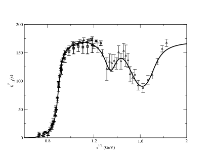
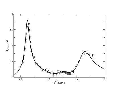
Figure 11: $\phi_{11}$ (top) and $|t_{11}|$ (bottom) of $K\pi\rightarrow K\pi$ scattering amplitude vs data from Mercer:1971 (squares), Estabrooks:1978 (circles), and Aston:1988 (triangles).

We can express $\hat{t}_{\alpha\beta}=t_{\alpha\beta}/(4q_{\alpha}q_{\beta})$ in terms of a product of poles, zeros and the Omnés-Muskhelishvili function

$$\hat{t}_{\alpha\beta}=N_{\alpha\beta}\frac{\prod_{l=1,N_{z,\alpha\beta}}(s-s^{(\alpha\beta)}_{z,l})}{\prod_{l=1,8}(s-s_{P,l})}$$ (71)

$$\times \exp\left(\frac{s}{\pi}\int_{(m_{K}+m_{\pi})^{2}}^{\infty}ds^{\prime}\frac{\phi_{\alpha\beta}(s^{\prime})}{s^{\prime}(s^{\prime}-s)}\right).$$

where $N_{z,\alpha\beta}$ is the number of zeros of $\hat{t}_{\alpha\beta}$ for which we find $N_{z,11}=N_{z,22}=7$, $N_{z,12}=N_{z,21}=6$. The normalization factors are given by $N_{11}=7.075,N_{12}=-421.989,N_{22}=2.808$. The positions of the poles and zeros are given by (in units of $\mbox{GeV}^{2}$)

$$s_{P,1/2}=0.3573\pm i0.4055,\ \ s_{P,3/4}=2.4912\pm i0.5762,$$

$$s_{P,5/6}=20.3504\pm i3.3856,$$

$$s_{P,7}=-0.00489,\ \ s_{P,8}=-6.2666,$$ (72)

and

$$s^{(11)}_{z,1/2}=0.3428\pm i0.4470,\ \ s^{(11)}_{z,3/4}=2.2188\pm i0.6175,$$

$$s^{(11)}_{z,5/6}=12.8061\pm i0.2470,\ \ s^{(11)}_{z,7}=0.$$

$$s^{(12)}_{z,1/2}=1.9181\pm i0.3669,\ \ s^{(12)}_{z,3}=3.3956,$$

$$s^{(12)}_{z,4}=M_{K^{*}(892)}^{2},\ \ s^{(11)}_{z,5/6}=0.$$

$$s^{(22)}_{z,1/2}=2.2704\pm i0.2273,\ \ s^{(22)}_{z,3/4}=20.2775\pm i3.3479,$$

$$s^{(22)}_{z,5}=-0.00489,\ \ s^{(22)}_{z,6}=-6.1874,\ \ s^{(22)}_{z,7}=0,$$

respectively. As can be seen from Fig. 12, this $K$-matrix leads to a dramatic, most likely unphysical, drop in the phase $\phi_{11}$ (dashed line) around $6\mbox{ GeV}^{2}$ and this results in both $\phi_{11}$ and $\delta_{11}$ vanishing asymptotically. Furthermore the resulting t-matrix has complex poles and zeros on the physical sheet (see Eq. (B.1) and Eq. (B.1)). The origin of these unphysical poles can be illustrated by considering a single channel, $K_{11}$ only, with a single pole and constant background term. The resulting $t$-matrix element is then given by,

$$\hat{t}_{11} = \frac{1}{8}\frac{\alpha_{1}^{2}+\gamma^{0}_{11}(M_{K^{*}(892)}^{2}-s)}{(M_{K^{*}(892)}^{2}-s)-\frac{[s-(m_{K}-m_{\pi})^{2}][s-(m_{K}+m_{\pi})^{2}]}{s}I_{1}(s)[\alpha_{1}^{2}+\gamma^{0}_{11}(M_{K^{*}(892)}^{2}-s)]}.$$ (74)

If, for simplicity, we replace $m_{K}$ by $m_{\pi}$ and keep only the imaginary of $I_{1}(s)$, in the limit $|s|\rightarrow\infty$ and $\gamma^{0}_{11}\rightarrow 0$ with $|\gamma^{0}_{11}||s|\gg\alpha_{1}^{2}$ one finds

$$\hat{t}_{11} \rightarrow \frac{1}{8}\frac{\gamma^{0}_{11}}{1-i\sqrt{1-\frac{4m_{\pi}^{2}}{s}}\gamma^{0}_{11}s}.$$ (75)

In the limit $\gamma^{0}_{11}\rightarrow 0$ the pole is on the first sheet and approaches $s\rightarrow\pm\frac{i}{\gamma^{0}_{11}}$. Even though the K-matrix itself has unphysical singularities and zeros it still faithfully reproduces the phase and magnitude of the amplitude of $K\pi$ scattering data up to $1.8\mbox{ GeV}$. Similarly to the cases in $\pi\pi$ and $K\bar{K}$ scattering presented in previous sections, we will truncate the K-matrix solution at $s_{low}$ and match it with Regge parameterization at $s_{high}$.

B.2 Regge parameterization for $\pi^{0}K^{\pm}\rightarrow\pi^{0}K^{\pm}$ ($s>s_{high}$)

Asymptotically we only retain Pomeron ($P$) in the t-channel and the $K^{*}$ trajectory in the u-channel

$$F^{I_{t}=0}_{\pi K\rightarrow\pi K}(t,s,u)$$

$$= -\frac{1+e^{-i\pi\alpha_{P}(t)}}{\sin\pi\alpha_{P}(t)}\beta^{\pi K}_{P}\alpha_{P}(t)\frac{1+\alpha_{P}(t)}{2}e^{bt}(s/\hat{s})^{\alpha_{P}(t)}.$$

$$F^{I_{u}=\frac{1}{2}}_{\pi K\rightarrow\pi K}(u,t,s)$$

$$= \frac{1-e^{-i\pi\alpha_{K^{*}}(u)}}{\sin\pi\alpha_{K^{*}}(u)}\beta_{K^{*}}\frac{2\alpha_{K^{*}}(u)+1}{2\alpha_{K^{*}}(0)+1}e^{bu}(\alpha^{\prime}_{K^{*}}s)^{\alpha_{K^{*}}(u)}.$$

The Pomeron trajectory is given in Eq. (A.2) with parameters in Pomeron parameterization are taken from pelaez:2005 ; pelaez:2004 , except the coupling constant $\beta^{\pi K}_{P}=f^{(P)}_{\pi}f^{(P)}_{K}=[\beta_{P}^{\pi\pi}\beta_{P}^{K\bar{K}}]^{\frac{1}{2}}=1.709$. The $K^{*}$ trajectory is given by $\alpha_{K^{*}}(u)=0.352+0.882u$ as in Section A.2. From s-t and s-u channel crossing, we obtain

$$F^{I_{s}=\frac{1}{2}}_{\pi K\rightarrow\pi K}(s,t,u)$$

$$= \frac{1}{\sqrt{6}}F^{I_{t}=0}_{\pi K\rightarrow\pi K}(t,s,u)+F^{I_{t}=1}_{\pi K\rightarrow\pi K}(t,s,u)$$

$$+ \frac{1}{3}F^{I_{u}=\frac{1}{2}}_{\pi K\rightarrow\pi K}(u,t,s)+\frac{4}{3}F^{I_{u}=\frac{3}{2}}_{\pi K\rightarrow\pi K}(u,t,s).$$

The $P$-wave projection of the Regge amplitude in $\pi K\rightarrow\pi K$ scattering is given by

$$t^{Regge}_{\pi K\rightarrow\pi K}(s)=\frac{\pi}{8}\int_{-1}^{1}(d\cos)\cos\theta$$ (79)

$$\times [\frac{1}{\sqrt{6}}F^{I_{t}=0}_{\pi K\rightarrow\pi K}(t,s,u)+\frac{1}{3}F^{I_{u}=\frac{1}{2}}_{\pi K\rightarrow\pi K}(u,t,s)].\ \ \ \ \ \ \ \$$

The complete amplitude for the $\pi K\rightarrow\pi K$ amplitude is given by,

$$t_{\pi K\rightarrow\pi K}(s)=\left\{\begin{array}[]{c}t_{11}^{Kmatrix}(s),s<s_{low}\\ t_{\pi K\rightarrow\pi K}^{Regge}(s),s>s_{high}\end{array}\right.\ \ \ \ \ \ \ \$$ (82)

where we choose $\sqrt{s_{low}}=2.3$GeV, $\sqrt{s_{high}}=2.5$GeV for the real part of the amplitude and $\sqrt{s_{high}}=2.7$GeV for the imaginary part of the amplitude as shown in Fig. 12.

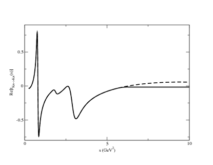
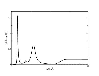
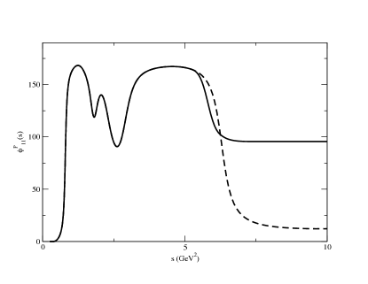
Figure 12: Real (left) and imaginary (right) parts of the isovector, $P$-wave amplitude, $t_{\pi K\rightarrow\pi K}(s)$ and phase $\phi_{11}$ (solid curves). The dashed curves are the result of the $K$-matrix parameterization.

From the $P$-wave projection of the Regge amplitude we find the following asymptotic behavior for the phase $\phi_{11}(s)$ and denominator function of the complete amplitudes,

$$\phi_{11}\rightarrow\arctan[-\frac{\sin\pi\alpha_{P}(0)}{1+\cos\pi\alpha_{P}(0)}]=\frac{\pi}{2},$$

$$\frac{1}{D_{\pi K\rightarrow\pi K}(s)}\rightarrow\frac{i}{s^{\frac{1}{2}}}$$ (83)

The phase is shown in Fig. 12,

References

- (1) B. Diekmann, Phys. Rep. 159, 99 (1988).
- (2) B. Hyams, C. Jones and P. Weilhammer, Nucl. Phys. B 64, 134 (1973).
- (3) D. Aston et al., Phys. Lett. B 92, 215 (1980).
- (4) D. Bisello et al., Phys. Lett. B 220, 321 (1989).
- (5) A. Donnachie and H. Mirzaie, Z. Phys. C 33, 407 (1987).
- (6) J. J. Dudek, R. G. Edwards, M. J. Peardon, D. G. Richards, and C. E. Thomas, Phys. Rev. D 82, 034508 (2010).
- (7) S. Godfrey and N. Isgur , Phys. Rev. D 32, 189 (1985).
- (8) K. Nakamura et al. (Particle Data Group), J. Phys. G 37, 075021 (2010).
- (9) N.N.Achasov and A.A.Kozhevnikov , Phys. Atom. Nucl. 60, 1011 (1997).
- (10) N.N.Achasov and A.A.Kozhevnikov , Phys. Atom. Nucl. 65, 153 (2002).
- (11) P. Guo, R. Mitchell and A. P. Szczepaniak, Phys. Rev. D 82, 094002 (2010).
- (12) BES Collaboration (M. Ablikim et al.), Phys. Rev. Lett. 97, 142002 (2006).
- (13) X. Liu, B. Zhang, L.-L. Shen, and S.-L. Zhu, Phys. Rev. D 75, 074017 (2007).
- (14) B. A. Li, Phys. Rev. D 76, 094016 (2007).
- (15) A. P. Szczepaniak, P. Guo, M. Battaglieri and R. De Vita, Phys. Rev. D 82, 036006 (2010)
- (16) S.D. Protopopescu et al. , Phys. Rev. D 7, 1279 (1973).
- (17) P. Estabrooks and A. D. Martin, Nucl. Phys. B 79, 301 (1974).
- (18) T. N. Pham and T. N. Truong, Phys. Rev. D 16, 896 (1977).
- (19) D. Aston et al., Nucl. Phys. B 296, 493 (1988).
- (20) R. Mercer et al., Nucl. Phys. B 32, 381 (1971).
- (21) P. Estabrooks et al., Nucl. Phys. B 133, 490 (1978).
- (22) J. R. Pel ez and F. J. Yndur in , Phys. Rev. D 69, 114001 (2004).
- (23) B. Ananthanarayan, G. Colangelo, J. Gasser and H. Leutwyler , Phys. Rep. 353, 207 (2001).
- (24) J. R. Pel ez and F. J. Yndur in , Phys. Rev. D 71, 074016 (2005).
- (25) B. Ananthanarayan, P. B ttiker and B. Moussallam , Eur. Phys. J. C 22, 133 (2001).
- (26) D. H. Cohen, D.S. Ayres, R. Diebold, S.L. Kramer, A.J. Pawlicki and A.B. Wicklund , Phys. Rev. D 22, 2595 (1980).