Error correction during DNA replication

Abstract

DNA polymerase (DNAP) is a dual-purpose enzyme that plays two opposite roles in two different situations during DNA replication. It plays its normal role as a polymerase catalyzing the elongation of a new DNA molecule by adding a monomer. However, it can switch to the role of an exonuclease and shorten the same DNA by cleavage of the last incorporated monomer from the nascent DNA. Just as misincorporated nucleotides can escape exonuclease causing replication error, correct nucleotide may get sacrificed unnecessarily by erroneous cleavage. The interplay of polymerase and exonuclease activities of a DNAP is explored here by developing a minimal stochastic kinetic model of DNA replication. Exact analytical expressions are derived for a few key statistical distributions; these characterize the temporal patterns in the mechanical stepping and the chemical (cleavage) reaction. The Michaelis-Menten-like analytical expression derived for the average rates of these two processes not only demonstrate the effects of their coupling, but are also utilized to measure the extent of replication error and erroneous cleavage.

I Introduction

DNA polymerase (DNAP) replicates a DNA molecule; the sequence of the nucleotides, the monomeric subunit of DNA, on the product of polymerization is dictated by that on the corresponding template DNA through the Watson-Crick complimentary base-paring rule kornberg . DNAP moves step-by-step along the template strand utilizing chemical energy input and, therefore, these are also regarded as a molecular motor howard ; kolofisher .

An unique feature of DNAP is that it is a dual-purpose enzyme that plays two opposite roles in two different circumstances during DNA replication. It plays its normal role as a polymerase catalyzing the elongation of a new DNA molecule. However, upon committing an error by the misincorporation of a wrong nucleotide, it switches its role to that of a exonuclease catalyzing the shortening of the nascent DNA by cleavage of the misincorporated nucleotide at the growing tip of the elongating DNA krantz10 . The two distinct sites on the DNAP where, respectively, polymerization and cleavage are catalyzed, are separated by 3-4 nm ibarra09 . The nascent DNA is transferred back to the site of polymerization after cleaving the incorrect nucleotide from its growing tip. The elongation and cleavage reactions are thus coupled by the transfer of the DNA between the sites of polymerase and exonuclease activity of the DNAP. However, the physical mechanism of this transfer is not well understood xie09 .

In this paper we develop a minimal kinetic model of DNA replication (more precisely, that of the “leading strand” which can proceed continuously) that captures the coupled polymerase and exonuclease activities of a DNAP within the same theoretical framework. From this model, we derive the exact analytical expressions for (i) the dwell time distribution (DTD) of the DNAP at the successive nucleotides on the template DNA, and (ii) the distribution of the turnover times (DTT) of the exonuclease (i.e., the time intervals between the successive events of cleavage of misincorporated nucleotide from the nascent DNA). The mean of these two distributions characterize the average rates of elongation and cleavage, repectively; we show that both can be written as Michaelis-Menten-like expressions for enzymatic reactions which reveals the effect of coupling explicitly.

In our model, the kinetic pathways available to the correct and incorrect nucleotides are the same. However, it is the ratio of the rate constants that makes a pathway more favorable to one species than to the other. Similar assumption was made by Galas and Branscomb galas78 in one of the earliest models of replication. Therefore, in spite of the elaborate quality control system, some misincorporated nucleotides can escape cleavage; such replication error in the final product is usually about $1$ in $10^{9}$ nucleotides. Moreover, occasionally a correct nucleotide is erroneously cleaved unneccessarily; such “futile” cycles slow down replication fersht82 .

We define quantitative measures of these two types of error and derive their exact analytical expressions from our model for “wild type” DNAP. Using special cases of these analytical expressions, we also examine the effects of two different mutations of the DNAP ibarra09 - (i) “exo-deficient” mutant that is incapable of exonuclease activity, and (ii) “transfer-deficient” mutant on which the rate of transfer to the exonuclease site is drastically reduced.

II Model

Almost all DNAP share a common “right-hand-like” structure. Binding of the correct dNTP substrate triggers closing of the “hand” which is required for the formation of the diester bond between the recruited nucleotide monomer and the elongating DNA molecule. The kinetic scheme of our stochastic model of replication is shown in fig (1). The rate constants for the correct and incorrect nucleotides are denoted by $\omega$ and $\Omega$, respectively; the same subscript is used in both the cases for the same transition.

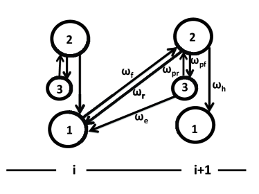
Figure 1: The kinetic model of DNA replication. The chemo-mechanical states of a single DNAP and the allowed transitions are shown along with the corresponding transition probabilities per unit time (the rate constants). The corresponding rate constants for the incorrect nucleotide are denoted by the symbol $\Omega$ (see the text for details).

Let us begin with the situation where the DNAP is ready to begin its next elongation cycle; these mechano-chemical state is labelled by the integer index $1$. In principle, the transition $1\to 2$ consists of two steps: binding of the dNTP substrate and the formation of the diester bond. The overall rate of this step is $\omega_{f}$ for a correct substrate and $\Omega_{f}$ for an incorrect substrate.

Occasionally, because of the random fluctuation of the “hand” between the “open” and “closed” conformations, the dNTP may escape even before the formation of the diester bond; this takes place with the rate constant $\omega_{r}$. If the recruited dNTP is incorrect, the hand remains “open” most of the time and the rate constant for the rejection of the dNTP is $\Omega_{r}$ ($\Omega_{r}>>\omega_{r}$). Note that dNTP selection through $1\rightleftharpoons 2$ involves a discrimination between the correct and incorrect dNTP substrate on the basis of free energy gained by complementary base-pairing with the template.

The transition $2(i+1)\to 1(i+1)$ corresponds to the relaxation of the freshly incorporated nucleotide to a conformation that allows the DNAP to be ready for the next cycle. The rate constants for this step are $\omega_{h}$ and $\Omega_{h}$ respectively, for correctly and incorrectly incorporated nucleotides. Alternatively, while in the state $2(i+1)$, the DNAP can transfer the growing DNA molecule to its exonuclease site; this transfer takes place at a rate $\omega_{pf}$ ($\Omega_{pf}$) if the selected nucleotide is correct (incorrect). Since $\Omega_{h}<<\omega_{h}$, and $\Omega_{pf}>>\omega_{pf}$, the misincorporated nucleotide most often gets transferred to the exonuclease site whereas relaxation, rather than transfer, is the most probable pathway when the incorporated nucleotide is correct.

The actual cleavage of the diester bond that severs the nucleotide at the growing tip of the DNA is represented by the transition $3(i+1)\to 1(i)$. For a correct nucleotide, $\omega_{pr}>>\omega_{e}$ indicating that the DNA is likely to be transferred back to the polymerase site without the unneccesary cleavage of the correct nucleotide. In contrast, for an incorrect nucleotide, $\Omega_{pr}<<\Omega_{e}$ which makes error correction a highly probable event. Moreover, $\Omega_{pr}<<\omega_{pr},\Omega_{e}>>\omega_{e}$.

Since the trimmed DNA is transferred to the polymerase site extremely rapidly krantz10 , each of the rate constants $\omega_{e}$ and $\Omega_{e}$ incorporate both the trimming and transfer.

Interestingly, the full kinetic scheme in fig.1 can be viewed as a coupling of a purely polymerase-catalyzed reaction (shown in the left panel of fig.2) and a purely exonuclease-catalyzed reaction (shown in the right panel of fig.2); the transition with the rate $\omega_{pr}$ couples these two reactions.

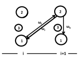
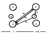
Figure 2: “Purely” polymerizing reaction (left panel) and “pure” exonuclease reaction (right panel).

Strictly speaking, for an “exo-deficient” DNAP ibarra09 , $\omega_{e}=0=\Omega_{e}$ although the rates of forward and reverse transfer between the sites of polymerase and exonuclease activities may not be necessarily negligible. Similarly, either $\omega_{pf}=0=\Omega_{pf}$, or $\omega_{pr}=0=\Omega_{pr}$ (or, both) can be the cause of “transfer-deficiency” of the DNAP.

III Results and discussion

III.1 Distribution of Dwell time

The DTD considered here arises from intrinsic stochasticity and not caused by any sequence inhomogeneity of the mRNA template schwartz11 . For a molecular motor that is allowed to step backward as well as forward, we use positive ($+$) and negative ($-$) signs to represent the forward and backward steps, respectively. For example, $\psi_{+-}(t)$ is the conditional DTD (cDTD) garai11 when a forward step is followed by a backward step and $p_{+-}$ is the probability of such a transition. Therefore, the DTD can be written as

$$\psi(t)=p_{+-}\psi_{+-}(t)+p_{++}\psi_{++}(t)+p_{-+}\psi_{-+}(t)+p_{--}\psi_{--}(t)$$ (1)

Since in our model two consecutive backward steps are forbidden implies that $p_{--}\psi_{--}(t)=0$. We calculate the cDTD following the standard method chemla that has been used successfully earlier for the calculation of cDTD for some other motors (see, for example, ref.garai11 ).

Let $P_{\mu}(j,t)$ be the probability of finding the DNAP in the $\mu$-th ($\mu=1,2,3$) chemical state at the $j$-th site (i.e., at the discrete position $x_{j}$ ($j=\infty,...-1,0,1,...\infty$). Then master equations for $P_{\mu}(j,t)$ are

$$\dfrac{dP_{1}(j,t)}{dt} = -\omega_{f}P_{1}(j,t)+\omega_{r}P_{2}(j+1,t)+\omega_{h}P_{2}(j,t)$$ (2)

$$+ \omega_{e}P_{3}(j+1,t)$$

$$\dfrac{dP_{2}(j,t)}{dt} = \omega_{f}P_{1}(j-1,t)-(\omega_{r}+\omega_{pf}+\omega_{h})P_{2}(j,t)$$ (3)

$$+ \omega_{pr}P_{3}(j,t)$$

$$\dfrac{dP_{3}(j,t)}{dt}=\omega_{pf}P_{2}(j,t)-(\omega_{e}+\omega_{pr})P_{3}(j,t)$$ (4)

In terms of the Fourier transform

$$\bar{P}_{\mu}(q,t)=\sum_{j=-\infty}^{\infty}P_{\mu}(x_{j},t)e^{-iqx_{j}}$$ (5)

of $P_{\mu}(x_{j},t)$, the master equations can be written as a matrix equation

$$\dfrac{d}{dt}\bar{\textbf{P}}(q,t)=\textbf{M(q)}\bar{\textbf{P}}(q,t)$$ (6)

where $\bar{\textbf{P}}(q,t)$ is a column vector whose 3 components are $\bar{P}_{1}(q,t),\bar{P}_{2}(q,t),\bar{P}_{3}(q,t)$ and

$$\textbf{M(q)}=\begin{bmatrix}-\omega_{f}&\omega_{h}+\omega_{r}\rho_{-}(q)&\omega_{e}\rho_{-}(q)\\ \omega_{f}\rho_{+}(q)&-(\omega_{h}+\omega_{r}+\omega_{pf})&\omega_{pr}\\ 0&\omega_{pf}&-(\omega_{e}+\omega_{pr})\end{bmatrix}$$ (7)

with $\rho_{+}(q)=e^{-iqd}$ and $\rho_{-}(q)=e^{iqd}$; $d$ being the step size, ie., $x_{j+1}-x_{j}=d$.

Taking Laplace transform of (6) with respect to time

$$\tilde{P}_{\mu}(q,s)=\int_{0}^{\infty}\bar{P}_{\mu}(q,t)e^{-st},$$ (8)

the solution of the master equation in the Fourier-Laplace space is

$$\tilde{{\bf P}}(q,s)={\bf R}(q,s)^{-1}\tilde{{\bf P}}(0)$$ (9)

where

$${\bf R}(q,s)=s{\bf I}-{\bf M}(q)$$ (10)

and $\tilde{{\bf P}}(0)$ is the column vector corresponding to the initial probabilities.

Now we define

$$\tilde{P}(q,s)=\sum\limits_{i=1}^{3}\tilde{P}_{i}(q,s)$$ (11)

which can be calculated from

$$\tilde{P}(q,s)=\dfrac{\sum\limits_{i,j=1}^{3}Co_{j,i}P_{j}(0)}{\lvert{\textbf{R}}(q,s)\rvert}$$ (12)

where $Co_{j,i}$ are the cofactors of the R(q,s).

The determinant of the matrix R(q,s) is a third order polynomial of $s$ and can be expressed as

$$\lvert{\textbf{R}}(q,s)\rvert=s^{3}+\alpha s^{2}+\beta(q)s+\gamma(q)$$ (13)

Note that $\alpha$ is independent of $q$ whereas $\beta$ and $\gamma$ are the function of $q$. For the explicit form (7) of ${\bf M}$ the coefficients $\alpha$, $\beta(q)$ and $\gamma(q)$ are given below.

$$\alpha=\omega_{e}+\omega_{f}+\omega_{h}+\omega_{pf}+\omega_{pr}+\omega_{r}$$ (14)

$\beta$ can be expressed as

$$\beta(q)=\beta(0)+\beta_{+}(1-\rho_{+}(q))+\beta_{+-}(1-\rho_{+}(q)\rho_{-}(q))$$ (15)

where

$$\beta(0) = \omega_{e}\omega_{f}+\omega_{e}\omega_{h}+\omega_{e}\omega_{pf}+\omega_{f}\omega_{pf}+\omega_{f}\omega_{pr}$$ (16)

$$+ \omega_{h}\omega_{pr}+\omega_{e}\omega{r}+\omega_{pr}\omega_{r}$$

$$\beta_{+}=\omega_{f}\omega_{h}$$ (17)

and

$$\beta_{+-}=\omega_{f}\omega_{r}.$$ (18)

Similarly,

$$\gamma(q)=\gamma_{+}(1-\rho_{+}(q))+\gamma_{+-}(1-\rho_{+}(q)\rho_{-}(q))$$ (19)

where

$$\gamma_{+}=\omega_{e}\omega_{f}\omega_{h}+\omega_{f}\omega_{h}\omega_{pr}$$ (20)

and

$$\gamma_{+-}=\omega_{e}\omega_{f}\omega_{pf}+\omega_{e}\omega_{f}\omega_{r}+\omega_{f}\omega_{pr}\omega_{r}$$ (21)

For convenience, we define the $2\times 2$ diagonal matrix

$$\mathbf{\rho(q)}=\begin{bmatrix}\rho_{+}(q)&0\\ 0&\rho_{-}(q)\end{bmatrix}$$ (22)

the column vector

$$\mathbf{\Psi(s)}=\dfrac{1}{s}\begin{bmatrix}1-p_{++}\psi_{++}(s)-p_{+-}\psi_{+-}(s)\\ 1-p_{-+}\psi_{-+}(s)-p_{--}\psi_{--}(s)\\ \end{bmatrix}$$ (23)

and the $2\times 2$ matrix

$$\mathbf{\psi(s)}=\begin{bmatrix}p_{++}\psi_{++}(s)&p_{+-}\psi_{+-}(s)\\ p_{-+}\psi_{-+}(s)&p_{--}\psi_{--}(s)\\ \end{bmatrix}$$ (24)

where $\psi_{\pm\pm}(s)$ are the Laplace transforms of the cDTDs $\psi_{\pm\pm}(t)$.

$\tilde{P}(q,s)$ and cDTD are related chemla by the equation

$$\tilde{P}(q,s)=\textbf{p}_{0}^{T}(\textbf{I}-\mathbf{\psi}(s)\mathbf{\rho}(q))^{-1}\mathbf{\Psi}(s)$$ (25)

where $\textbf{p}_{0}$ is the vector of initial conditions. For example, $\textbf{p}_{0}^{T}=(1~{}0)$ corresponds to the given condition that the motor has taken the initial step in the forward (+) direction.

Thus, in principle, if one can calculate $\tilde{P}(q,s)$, one can use the relation (25) to solve for $\psi_{\pm\pm}(s)$ and, then taking inverse Laplace transform, obtained $\psi_{\pm\pm}(t)$. To calculate $\tilde{P}(q,s)$, one has to use an appropriate set of initial conditions consistent with the defnition of the dwell times. The set $P_{1}=0$,$P_{2}=1$,$P_{3}=0$ ensures that first step is taken forward. In other words, in our calculation, we start the clock by setting it to $t=0$ when the DNAP reaches the state $2$ at $j$ from state $1$ at $j-1$. Therefore, in this case $p_{--}=0=p_{-+}$. Corresponding to this initial condition, we now define,

$$\tilde{P}_{+}(q,s)=\left.\tilde{P}(q,s)\right|_{\{P_{1}(0)=0,P_{2}(0)=1,P_{3}(0)=0\}}$$ (26)

and, from equation (25), we get chemla

$$\left.\dfrac{1}{s\tilde{P}_{+}(q,s)}\right|_{\{\rho_{-}(q)=0\}}=\dfrac{1-\rho_{+}(q)p_{++}\tilde{\psi}_{++}(s)}{1-p_{++}\tilde{\psi}_{++}(s)-p_{+-}\tilde{\psi}_{+-}(s)}$$ (27)

Equation (27) can be re expressed as

$$\left.\dfrac{1}{s\tilde{P}_{+}(q,s)}\right|_{\{\rho_{-}(q)=0\}}=a_{0}+a_{+}\rho_{+}(q)$$ (28)

where

$$a_{0} = \dfrac{1}{1-p_{++}\tilde{\psi}_{++}(s)-p_{+-}\tilde{\psi}_{+-}(s)}$$

$$a_{+} = -\dfrac{p_{++}\tilde{\psi}_{++}(s)}{1-p_{++}\tilde{\psi}_{++}(s)-p_{+-}\tilde{\psi}_{+-}(s)}$$ (29)

Hence,

$$p_{++}\tilde{\psi}_{++}(s)=-\frac{a_{+}}{a_{0}}$$ (30)

and

$$p_{+-}\tilde{\psi}_{+-}(s)=\frac{a_{0}+a_{+}-1}{a_{0}}$$ (31)

Therefore, next we obtain $\left.\dfrac{1}{s\tilde{P}_{+}(q,s)}\right|_{\{\rho_{-}(q)=0\}}$ directly from (12) and, by comparing it with equation (28), find out the expressions for $a_{0}$ and $a_{+}$; substituting these expressions for $a_{0}$ and $a_{+}$ into equations (30) and (31) we get $p_{++}\tilde{\psi}_{++}(s)$ and $p_{+-}\tilde{\psi}_{+-}(s)$, respectively.

Using the same initial condition, from equation (12), we get

$$\tilde{P}_{+}(q,s) = \dfrac{s^{2}+s(\alpha-\omega_{r}(1-\rho_{-}(q))+\beta(0)-(1-\rho_{-}(q))(\omega_{e}\omega_{pf}+\omega_{e}\omega_{r}+\omega_{pr}\omega_{r})}{s^{3}+\alpha s^{2}+\beta(q)s+\gamma(q)}$$

Therefore,

$$\left.\dfrac{1}{s\tilde{P}_{+}(q,s)}\right|_{\{\rho_{-}(q)=0\}}=\dfrac{s^{3}+\alpha s^{2}+s(\beta(0)+\beta_{+}+\beta_{+-})+\gamma_{+}+\gamma_{+-}-(s\beta_{+}+\gamma_{+})\rho_{+}(q)}{s^{3}+s^{2}(\alpha-\omega_{r})+s(\beta(0)-(\omega_{e}\omega_{pf}+\omega_{e}\omega_{r}+\omega_{pr}\omega_{r}))}$$ (33)

Comparing equation (33) with equation (28) we identify $a_{0}$ and $a_{+}$ and substituting these expressions for $a_{0}$ and $a_{+}$ into (30) we get

$$p_{++}\tilde{\psi}_{++}(s)=\dfrac{s\beta_{+}+\gamma_{+}}{s^{3}+\alpha s^{2}+s(\beta(0)+\beta_{+}+\beta_{+-})+\gamma_{+}+\gamma_{+-}}=\dfrac{s\beta_{+}+\gamma_{+}}{(s+\omega_{1})(s+\omega_{2})(s+\omega_{3})}$$ (34)

where $\omega_{1}$,$\omega_{2}$ and $\omega_{3}$ are roots of the following equation

$$\omega^{3}-\alpha\omega^{2}+\omega(\beta(0)+\beta_{+}+\beta_{+-})-(\gamma_{+}+\gamma_{+-})=0$$ (35)

Inverse Laplace transformation of equation (34) gives the exact expression of $p_{++}\psi_{++}(t)$

$$p_{++}\psi_{++}(t)=\dfrac{e^{-\omega_{1}t}(\gamma_{+}-\beta_{+}\omega_{1})}{(\omega_{1}-\omega_{2})(\omega_{1}-\omega_{3})}+\dfrac{e^{-\omega_{2}t}(\gamma_{+}-\beta_{+}\omega_{2})}{(\omega_{2}-\omega_{1})(\omega_{2}-\omega_{3})}+\dfrac{e^{-\omega_{3}t}(\gamma_{+}-\beta_{+}\omega_{3})}{(\omega_{3}-\omega_{1})(\omega_{3}-\omega_{2})}$$ (36)

Similarly, using the expressions of $a_{0}$ and $a_{+}$ in eq. (31), we get

$$p_{+-}\tilde{\psi}_{+-}(s)=\dfrac{s^{2}\omega_{r}+s(\beta_{+-}+\omega_{e}\omega_{pf}+\omega_{e}\omega_{r}+\omega_{pr}\omega_{r})+\gamma_{+-}}{s^{3}+\alpha s^{2}+s(\beta(0)+\beta_{+}+\beta_{+-})+\gamma_{+}+\gamma_{+-}}$$ (37)

Inverse Laplace transformation gives the exact expression of $p_{+-}\psi_{+-}(t)$

$$p_{+-}\psi_{+-}(t)=\dfrac{e^{-\omega_{1}t}(\gamma_{+-}-c_{1}\omega_{1}+\omega_{1}^{2}\omega_{r})}{(\omega_{1}-\omega_{2})(\omega_{1}-\omega_{3})}+\dfrac{e^{-\omega_{2}t}(\gamma_{+-}-c_{1}\omega_{2}+\omega_{2}^{2}\omega_{r})}{(\omega_{2}-\omega_{1})(\omega_{2}-\omega_{3})}+\dfrac{e^{-\omega_{3}t}(\gamma_{+-}-c_{1}\omega_{3}+\omega_{3}^{2}\omega_{r})}{(\omega_{3}-\omega_{1})(\omega_{3}-\omega_{2})}$$ (38)

Note that by putting $s=0$ in equation (34) and (37) we get the “branching probabilities”

$$p_{++}=\dfrac{\gamma_{+}}{\gamma_{+}+\gamma_{+-}}$$ (39)

$$p_{+-}=\dfrac{\gamma_{+-}}{\gamma_{+}+\gamma_{+-}}$$ (40)

which satisfy the normalization condition $p_{++}+p_{+-}=1$. The cDTDs $\psi_{+-}(t)$ and $\psi_{++}(t)$ are plotted in figs. 3 and 4, respectively, for a few different values of the parameters $\omega_{r}$ and $\omega_{f}$. In both the figures, the most probable dwell time increases with decreasing $\omega_{r}$ and decreasing $\omega_{f}$.

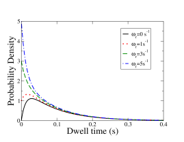
Figure 3: (Color online) Probability density of conditional dwell time, $\psi_{+-}$(t) is plotted for a few different values of parameter $\omega_{r}$. The values of other parameters are (all in $s^{-1}$) $\omega_{f}$=20.0, $\omega_{pf}$=30.0, $\omega_{pr}$=15.0, $\omega_{h}$=40.0 and $\omega_{e}=$4.0.

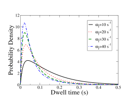
Figure 4: (Color online) Probability density of conditional dwell time, $\psi_{++}$(t) is plotted for a few different values of parameter $\omega_{f}$. The values of other parameters are (all in $s^{-1}$) $\omega_{r}$=5.0, $\omega_{pf}$=30.0, $\omega_{pr}$=15.0, $\omega_{h}$=40.0 and $\omega_{e}=4.0$.

In the same matrix-based formalism, the average velocity of a DNAP is given by the general expression chemla

$$V_{p}=-i\dfrac{\dot{\gamma}(0)}{\beta(0)},$$ (41)

where the dot indicates derivative with respect to $q$. The right hand side of eqn.(41) can be evaluated for our model of DNAP using the explicit expressions (19) and (16) for $\gamma(q)$ and $\beta(0)$, respectively. For the purpose of showing close relation of $V$ with the Michaelis-Menten (MM) equation for the average rates of enzymatic reaction, we now assume that dNTP binding is rate limiting (the general framework of our theory does not need this assumption). Under this assumption, we can write

$$\omega_{f}=\omega_{f}^{0}[dNTP_{c}]~{}{\rm and}~{}\Omega_{f}=\Omega_{f}^{0}[dNTP_{w}]$$ (42)

where $[dNTP_{c}]$ and $[dNTP_{w}]$ are the concentrations of the correct and incorrect substrates, respectively, and that $\omega_{f}^{0}>>\Omega_{f}^{0}$. In this case, the average velocity of the DNAP, i.e., the average rate of polymerization, can be expressed in a MM-like form

$$V_{p}^{(c)}=\dfrac{\tilde{K}_{cat}[dNTP_{c}]}{\tilde{K}_{M}+[dNTP_{c}]}$$ (43)

for the correct nucleotides, where

$$\tilde{K}_{cat}=\dfrac{\omega_{h}(\omega_{e}+\omega_{pr})}{\omega_{pr}+\omega_{e}+\omega_{pf}}$$ (44)

and the effective Michaelis constant is

$$\tilde{K}_{M}=\dfrac{(\omega_{pr}+\omega_{e})(\omega_{h}+\omega_{r})+\omega_{pf}\omega_{e}}{\omega_{f}^{0}(\omega_{pr}+\omega_{e}+\omega_{pf})}$$ (45)

Replacing $\omega$ by $\Omega$ and $[dNTP_{c}]$ by $[dNTP_{w}]$ we get the average rate of polymerization $V_{p}^{w}$ for the wrong nucleotides. In the limit of negligible exonuclease activity, the kinetic diagram shown in fig.1 reduces to the scheme shown on the left panel of fig.2 which is the standard MM-scheme with a single intermediate complex; in this limit the expressions for $\tilde{K}_{cat}$ and $\tilde{K}_{M}$ are consistent with those for the standard MM scheme enzymebook .

III.2 Distribution of turnover time for exonuclease

In this section we derive the DTT for exonuclease activity of the DNAP. We insert a hypothetical state $P_{1}^{*}$ such that

$$P_{3}\overset{\omega_{e}}{\rightarrow}P_{1}^{*}\overset{\delta}{\rightarrow}P_{1}$$ (46)

where in the limit $\delta\rightarrow\infty$, $P_{1}$ and $P^{*}_{1}$ become identical and we recover our original model.
For the simplicity of notation, in this subsection we drop the site index without loss of any information. The master equations for $P_{\mu}(t)$ ($\mu=1,2,3$) and that for $P_{1}^{*}(t)$ are

$$\dfrac{dP_{1}(t)}{dt} = -\omega_{f}P_{1}(t)+(\omega_{r}+\omega_{h})P_{2}(t)$$ (47)

$$\dfrac{dP_{2}(t)}{dt} = \omega_{f}P_{1}(t)-(\omega_{r}+\omega_{pf}+\omega_{h})P_{2}(t)$$ (48)

$$+ \omega_{pr}P_{3}(t)$$

$$\dfrac{dP_{3}(t)}{dt}=\omega_{pf}P_{2}(t)-(\omega_{e}+\omega_{pr})P_{3}(t)$$ (49)

$$\dfrac{dP_{1}^{*}(t)}{dt}=\omega_{e}P_{3}(t)$$ (50)

For the calculation of DTT, we impose the initial condition $P_{1}(0)=1$, and $P_{2}(0)=P_{3}(0)=P_{1}^{*}(0)=0$. Suppose, $f(t)$ denotes the DTT. Then, $f(t)~{}\Delta t$ is the probability that one exonuxlease cycle is completed between $t$ and $t+\Delta t$, i.e., the DNAP was in state 3 at time $t$ and made a transition to the state $1*$ between $t$ and $t+\Delta$. Obviously, $f(t)\Delta t=\omega_{e}P_{3}(t)$ and, hence,

$$f(t)=\omega_{e}P_{3}(t)$$ (51)

Using a compact matrix notation, the equations (47),(48) and (49) can be written the form

$$\dfrac{d}{dt}{\textbf{Q}}(t)=\textbf{N}{\textbf{Q}}(t)$$ (52)

where

$$\textbf{N}=\begin{bmatrix}-\omega_{f}&\omega_{h}+\omega_{r}&0\\ \omega_{f}\ &-(\omega_{h}+\omega_{r}+\omega_{pf})&\omega_{pr}\\ 0&\omega_{pf}&-(\omega_{e}+\omega_{pr})\end{bmatrix}$$ (53)

and

$$\textbf{Q}=\begin{bmatrix}P_{1}(t)\\ P_{2}(t)\\ P_{3}(t)\end{bmatrix}$$ (54)

Solution of the equation (52) in Laplace space

$$\tilde{\textbf{Q}}(s)=\textbf{S}(s)^{-1}\tilde{\textbf{Q}}(0)$$ (55)

where

$$\textbf{S}(s)=s\textbf{I}-\textbf{N}.$$ (56)

Solution (55) for the assumed initial conditions provide,

$$\tilde{P}_{3}(s)=\dfrac{(-1)^{1+3}\mathbf{Co}_{13}}{|\mathbf{S}(s)|}$$ (57)

which, explicitly in terms of the rate constants, takes the form

$$\tilde{P}_{3}(s)=\dfrac{\omega_{f}\omega_{pf}}{s^{3}+\alpha^{\prime}s^{2}+\beta^{\prime}s+\gamma^{\prime}}$$ (58)

where

$$\alpha^{\prime}=\omega_{e}+\omega_{f}+\omega_{h}+\omega_{pf}+\omega_{pr}+\omega_{r}$$ (59)

$$\beta^{\prime} = \omega_{f}\omega_{pf}+\omega_{e}\omega_{h}+\omega_{e}\omega_{pf}+\omega_{f}\omega_{pf}+\omega_{f}\omega_{pr}+\omega_{h}\omega_{pr}$$ (60)

$$+ \omega_{e}\omega_{pr}+\omega_{pr\omega_{r}}$$

$$\gamma^{\prime}=\omega_{f}\omega_{pf}\omega_{e}$$ (61)

Since in the Laplace space the equation (51) becomes

$$\tilde{f}(s)=\omega_{e}\tilde{P}_{3}(s),$$ (62)

we get

$$\tilde{f}(s)=\dfrac{\omega_{e}\omega_{f}\omega_{pf}}{s^{3}+\alpha^{\prime}s^{2}+\beta^{\prime}s+\gamma^{\prime}}=\dfrac{\omega_{e}\omega_{f}\omega_{pf}}{(s+\upsilon_{1})(s+\upsilon_{2})(s+\upsilon_{3})}$$ (63)

as the DTT in the Laplace space.

Taking the inverse Laplace transform of equation (63), we get the DTT

$$f(t)=\biggl{[}\dfrac{\omega_{f}\omega_{pf}\omega_{e}}{(\upsilon_{1}-\upsilon_{2})(\upsilon_{1}-\upsilon_{3})}\biggr{]}e^{-\upsilon_{1}t}+\biggl{[}\dfrac{\omega_{f}\omega_{pf}\omega_{e}}{(\upsilon_{2}-\upsilon_{1})(\upsilon_{2}-\upsilon_{3})}\biggr{]}e^{-\upsilon_{2}t}+\biggl{[}\dfrac{\omega_{f}\omega_{pf}\omega_{e}}{(\upsilon_{3}-\upsilon_{1})(\upsilon_{3}-\upsilon_{2})}\biggr{]}e^{-\upsilon_{3}t}$$ (64)

where $\upsilon_{1}$,$\upsilon_{2}$,$\upsilon_{3}$ are solution of the following equation

$$\upsilon^{3}-(\omega_{e}+\omega_{f}+\omega_{h}+\omega_{pf}+\omega_{pr}+\omega_{r})\upsilon^{2}+(\omega_{f}\omega_{pf}+\omega_{e}\omega_{h}+\omega_{e}\omega_{pf}+\omega_{f}\omega_{pf}+\omega_{f}\omega_{pr}+\omega_{h}\omega_{pr}+\omega_{e}\omega_{pr}+\omega_{pr\omega_{r}})\upsilon$$ (65)

$$- (\omega_{f}\omega_{pf}\omega_{e})=0.$$

This DTT is plotted in fig(5). Plots are consistent with the intuitive expectation that increasing $\omega_{pf}$ leads to a decrease the turnover time.

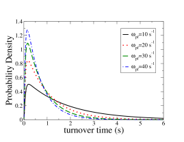
Figure 5: (Color online) Probability density of turnover time for unproductive exonuclease mode of enzyme, f(t) is plotted for a few different values of parameter $\omega_{pf}$. The values of the other parameters are (all in $s^{-1}$) $\omega_{f}$=20.0, $\omega_{r}$=5.0, $\omega_{pr}$=15.0, $\omega_{h}$=40.0 and $\omega_{e}=4.0$.

Suppose $\langle t\rangle$ denotes the mean time gap between the completition of the successive exonuclease reactions catalyzed by the DNAP. Then the average rate $V_{e}=1/\langle t\rangle$ of the exonuclease reaction can be expressed in a MM-like form kou05

$$V_{e}^{(c)}=\dfrac{K_{cat}[dNTP_{c}]}{K_{M}+[dNTP_{c}]}~{}{\rm with}~{}K_{cat}=\dfrac{\omega_{pf}\omega_{e}}{\omega_{e}+\omega_{pf}+\omega_{pr}}$$ (66)

for the correct nucleotides where $K_{M}=\tilde{K}_{M}$. Replacing $\omega$ by $\Omega$ and $[dNTP_{c}]$ by $[dNTP_{w}]$ in (66) we get $V_{e}^{(w)}$ for the wrong nucleotides. In the limit $\omega_{h}\to 0$, $\omega_{pr}\to 0$, the kinetic diagram shown in fig.1 reduces to the simpler scheme shown on the right panel of fig.2 which is essentially a generalized MM-like scheme with two intermediate states. Not surprisingly, in this limit, the average rate of the exonuclease reaction is consistent with that of the MM-like scheme with two intermediate states enzymebook .

III.3 Quantitative measures of error

Note that $\Phi_{p}=\tilde{V}_{p}^{(w)}/(\tilde{V}_{p}^{(w)}+\tilde{V}_{p}^{(c)})$ is the fraction of nucleotides misincorporated in the final product of replication. Similarly, the fraction $\Phi_{e}=V_{e}^{c}/(V_{e}^{c}+V_{e}^{w})$ is a measure of the errorneous severings, i.e., fraction of the cleaved nucleotides that were incorporated correctly into the growing DNA. Since $\omega_{pr}$ is the strength of the “coupling” between the two different enzymatic activities, we plot $\Phi_{p}$ and $\Phi_{e}$ against $\omega_{pr}$ in fig.6 for a few typical sets of values of the model parameters.

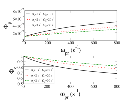
Figure 6: (Color online) $\Phi_{p}$ and $\Phi_{e}$ plotted against $\omega_{pr}$ while the ratio $\Omega_{pr}/\omega_{pr}=0.1$ is kept fixed. The three curves correspond to $\omega_{e}=1.0$s^-1, $2.0$s^-1, $3.0$s^-1. The values of the other pararemeters are (all in s^-1): $\omega_{f}=1.0$, $\Omega_{f}=10^{-5}$, $\omega_{pf}=0.1$, $\Omega_{pf}=10.0$, $\omega_{r}=.1$, $\Omega_{r}=1.0$, $\omega_{h}=10.0$, $\Omega_{h}=0.1$.

Decreasing $\Phi_{e}$ with increasing $\omega_{pr}$ is a consequence of the escape route via $\omega_{pr}$ for the correctly incorporated nucleotides that get transferred unnecessarily to the exonuclease site. It is the increasing number of such correctly incorporated nucleotides recused from the exonuclease site that leads to the lowering of $\Phi_{p}$ with increasing $\omega_{pr}$. The limiting values of $\Phi_{p}$ and $\Phi_{e}$ in the limit of large $\omega_{pr}$, are determined by the corresponding limiting expressions ${\tilde{V}}_{p}^{(c)}\simeq(\omega_{f}\omega_{h})/(\omega_{h}+\omega_{f}+\omega_{r})$, and $V_{e}^{(c)}\simeq(\omega_{f}\omega_{pf}\omega_{e})/[\omega_{pr}(\omega_{h}+\omega_{f}+\omega_{r})]$. (Expressions for ${\tilde{V}}_{p}^{(w)}$ and $V_{e}^{(w)}$ are similar in the limit of large $\Omega_{pr}$.)

IV Summary and conclusion

Here we have theoretically investigated the effects of the coupling of two different modes of enzymatic activities of a DNAP, in one of these it elongates a DNA whereas in the other it shortens the same DNA. The fundamental questions we have addressed here in the context of DNA replication have not been addressed by earlier theoretical works goel03 . The effects of tension on the polymerase and exonuclease activities, which have been the main focus of the earlier works goel03 , will be reported elsewhere sharma12 . The mechanism of error correction by DNAP is somewhat different from the mechanism of transcriptional proofreading which is intimately coupled to “back tracking” of the RNA polymerase voliotis09 ; sahoo11 .

We have derived exact analytical formulae for the cDTD and DTT which will be very useful in analyzing experimental data in single DNAP biophysics, particularly its stepping patterns and enzymatic turnover. In spite of their coupling, the average rates of both the enzymatic activities are MM-like; the analytical expressions for the effective MM parameters explicitly display the nature of the coupling of the two kinetic processes. We have also reported exact analytical expressions for the fractions $\Phi_{p}$ and $\Phi_{e}$ which measure replication error and erroneous cleavage; these expressions can be used for analyzing data from both single molecule ibarra09 and bulk wong91 experiments on wild type and mutant DNAPs.

Acknowledgements: We thank Stefan Klumpp for useful comments. This work has been supported at IIT Kanpur by the Dr. Jag Mohan Garg Chair professorship (DC) and a CSIR fellowship (AKS). This research (DC) has been supported in part also by the Mathematical Biosciences Institute at the Ohio State University and the National Science Foundation under grant DMS 0931642.

V Bibliography

References

• (1) A. Kornberg and T. baker, DNA replication, (Freeman, 1992).
• (2) J. Howard, Mechanics of motor proteins and the cytoskeleton (Sinauer Associates, 2001).
• (3) A.B. Kolomeisky and M.E. Fisher, Molecular motors: a theorist’s perspective, Annu. Rev. Phys. Chem. 58, 675 (2007).
• (4) L.J. Reha-Krantz, Biochim. Biophys. Acta 1804, 1049 (2010).
• (5) B. Ibarra, Y. R. Chemla, S. Plyasunov, S.B. Smith, J. M. Lazaro, M. Salas and C. Bustamante, EMBO J. 28, 2794 (2009)
• (6) P. Xie, J. Theor. Biol. 259, 434 (2009).
• (7) D.J. Galas and E.W. Branscomb, J. Mol. Biol. 124, 653 (1978).
• (8) A.R. Fersht, J.W.K. Jones and W.C. Tsui, J. Mol. Biol. 156, 37 (1982).
• (9) J.J. Schawrtz and S.R. Quake, PNAS 106, 20294 (2009).
• (10) A. Garai and D. Chowdhury, EPL 93, 58004 (2011).
• (11) Y. R. Chemala, J. R. Moffitt and C. Bustamante, J. Phys. Chem. B, 112, 6025 (2008)
• (12) M. Dixon and E.C. Webb, Enzymes (Academic Press, 1979).
• (13) S.C. Kou, B.J. Cherayil, W. Min, B.P. English and X.S. Xie, J. Phys. Chem. B 109, 19068 (2005).
• (14) A. Goel, R.D. Astumian and D. Herschbach, PNAS 100, 9699 (2003).
• (15) A.K. Sharma and D. Chowdhury, unpublished (2012).
• (16) M. Voliotis, N. Cohen, C. Molina-Paris and T.B. Liverpool, Phys. Rev. Lett 102, 258101 (2009).
• (17) M. Sahoo and S. Klumpp, EPL 96, 60004 (2011).
• (18) I. Wong, S.S. Patel and K.A. Johnson, Biochem. 30, 526 (1991).