A Multifrequency approach of the cosmological parameter estimation in presence of extragalactic point sources

Abstract

We present a multifrequency approach which optimizes the constraints on cosmological parameters with respect to extragalactic sources and secondary anisotropies contamination on small scales. We model with a minimal number of parameters the expected dominant contaminations in intensity, such as unresolved point sources and the thermal Sunyaev-Zeldovich effect. The model for unresolved point sources, either Poisson distributed or clustered, uses data from Planck early results. The overall amplitude of these contributions are included in a Markov Chain Monte Carlo analysis for the estimate of cosmological parameters. We show that our method is robust: as long as the main contaminants are taken into account the constraints on the cosmological parameters are unbiased regardless of the realistic uncertainties on the contaminants. We show also that the two parameters modelling unresolved points sources are not prior dominated.

1 Introduction

The CMB anisotropy data constitute a fundamental tool to test the standard cosmological model and its extensions. In particular small scale CMB anisotropies have a great importance in cosmology and are one of the current frontiers in CMB observations. Many experiments have been dedicated to the observations of small scale anisotropies. The Planck satellite (, 2005) will cover all the scales up to $\ell\sim 2500$ but there are also ground based experiments observing smaller regions of the sky but with higher angular resolutions, such as: ACBAR (, 2009), CBI (, 2004), QUaD (, 2009), SPT (, 2010), ACT (, 2011). At these scales, the Silk damping suppresses the primordial CMB contribution with respect to extragalactic contamination and secondary anisotropies. These contaminations affect the constraints on cosmological parameters derived from small scale data introducing biases and therefore it is necessary to properly account for them in the data analysis. We present an approach which has been developed to optimize, with respect to the contamination by point source contributions, the constraints on cosmological parameters which could be obtained from high resolution multi-frequency data.
The problem of extragalactic sources and secondary anisotropies contamination of the angular power spectrum and consequentely of the cosmological parameters has already been addressed in several recent articles (, 2006, 2008, 2009, 2009, 2011, 2011, 2011), together with the specific tools developed by the data analysis groups of the most recent small scale experiments (, 2011, 2011).

The approach we present in this article consists in modelling the astrophysical contributions to the angular power spectrum with minimal parametrizations, where minimal relates to the number of parameters necessary to describe the signals, and considering the frequency dependences of the different contributions. This is the most important difference with respect to previous approaches (, 2009, 2011, 2011, 2011, 2011). These parametrizations are included as additional contributions to the primary CMB in the Markov Chain MonteCarlo analysis to constrain cosmological parameters. The parameters characterizing the astrophysical contributions are included in the analysis together with the cosmological ones. As described in the following, we focus on the frequencies: $70,100,143,217,353$ GHz. We use the available data from Planck early results (, 2011a, b) to derive the parametrizations to describe the astrophysical signals. When no data are available, we rely on predictions from theoretical models and empirical simulations.

In the following, we use a fiducial cosmological model with the parameters from (2011) which are reported in the third column of Table 4. The polarization from point sources and SZ effect is negligible we thus do not take it into account. We also do not account for residual signal, in intensity nor in polarization, from our Galaxy.

The article is organized as follows. In Section 2 we describe the astrophysical signals and we derive the parametrizations of their contributions to the angular power spectrum. In Sect 3 we describe the analysis method and the frequency channel combinations. In Section 4 we present the results of the Markov Chain MonteCarlo (MCMC) analysis for the cosmological and astrophysical parameters. In section 5 we present the discussion and conclusions.

2 Astrophysical contaminations

One of the major contributions of astrophysical contamination on small scales, and in the regions of the sky clean from the Galactic emission, is given by discrete sources and in particular galaxy clusters and the extra-galactic point sources point sources. The former contributes through the Sunyaev Zeldovich (SZ) effect (, 1970,1980, 1972) whereas the latter contribution depends on the frequency. We have considered only the contribution of the thermal SZ effect since the kinetic SZ effect has a smaller amplitude. For the point-source contamination we considered different contributions depending on the frequency. We aim in this section at parametrising the different contributions by reducing to their minimum the number of parameters necessary to characterize the signals, and by including the frequency dependence in these parameters.

2.1 Thermal Sunyaev Zeldovich effect

The thermal SZ effect (TSZ) is a local spectral distortion of the CMB given by the interactions of CMB photons with the electrons of the hot gas in galaxy clusters (, 1970,1980) encountered during the propagation from the last scattering surface.

The TSZ contribution to the CMB signal strongly depends on the cosmological model and the cluster distribution through the dark matter halo mass function. It also depends on the cluster properties through the projected gas pressure profile. The TSZ angular power spectrum can be computed using these two ingredients (e.g. (2002, 2008)). It was shown in (2008) that the SZ contribution to the signal can be analysed in terms of a residual contribution to the total signal when the detected clusters are masked out from the maps, or in the contrary the TSZ signal can be analysed together with the CMB one without taking out the detected clusters providing the total SZ power spectrum is properly modelled, see (2009). The latter approach is the one that is used in the CMB experiments like WMAP (, 2011), ACT (, 2011, 2011) and SPT (, 2010, 2011). As discussed in (2009), we can consider three possible parametrizations for the TSZ power spectrum. However, the authors showed that the parametrization which represents physically the best the TSZ signal and at the same time does not bias the cosmological parameters is the one derived in (2002). It considers a template for the spectral shape, $\hat{C}_{\ell}$, and a normalisation which depends on the parameters $\sigma_{8}$ and $\Omega_{b}^{2}h^{2}$. According to these results, we chose to use:

$$C_{\ell}^{\mathrm{SZ}}(\nu)=A_{\mathrm{SZ}}g(\nu)\sigma_{8}^{7}\Omega_{\mathrm{b}}^{2}h^{2}\hat{C}_{\ell},$$ (2.1)

where $A_{\mathrm{SZ}}$ accounts for the uncertainty in the normalisation. The frequency dependence of the signal for the TSZ is given by the analytical function $g(\nu)$. In the following, we used a fiducial TSZ power-spectrum shape computed using the (2008) mass function and a pressure profile provided in (2009).

2.2 Point source contribution

An experiment like Planck with its moderate angular resolution is not optimized for point source detection. However, Planck, thanks to its full sky coverage and its 9 frequencies, is detecting a large number of sources with the detection thresholds reported in Table 1 and taken from (2011b). For the CMB analysis, the contribution of detected sources is removed by masking them in the maps. However, the contribution of unresolved point sources remains and needs to be properly dealt with since it acts like an unavoidable noise that impacts the angular power spectrum amplitude and the cosmological information contained in it.

In the frequency range of interest for our study the main contributions from extragalactic point sources are those of the radio galaxies which dominate the low frequency channels and the infrared ones which dominate the higher frequencies. Together with these two main populations there is a contribution from anomalous objects like Gigahertz Peaked Spectrum, Advection Dominated Accretion Flows/Adiabatic Inflow Outflow Solution and radio afterglows of Gamma Ray Burst (, 1998, 2005, 2005, 2006).

Radio galaxies, typically BL LACs and Flat Spectrum Radio Quasars present a flat spectrum $S_{\nu}\propto\nu^{\alpha}$ with $\alpha>{-0.5}$ (, 1987). There is also a contribution of steep spectra radio sources which typically have fluxes $S_{\nu}\propto\nu^{\alpha}$ with $\alpha\sim{-0.7-(-1)}$. The anomalous objects have only a minor contribution to the total of radio galaxy power at the arcmin scale (see for example (2005) for detailed discussion). Infrared galaxy emission presents a steep spectrum $S_{\nu}\propto\nu^{3.5}$ and is due to the UV light from star formation reprocessed by dust in galaxies. Infrared galaxies have been lengthly studied and observed in the recent past especially by CMB-dedicated experiments like ACT ((2011) and references therein), SPT (, 2010) and Planck (, 2011b) but also by Spitzer (, 2009), Blast (, 2009), and Herschel (, 2011).

In our range of frequencies and for our considered thresholds, the radio source contribution to the angular power spectrum can be described only by a Poissonian term. The situation is quite different for infrared galaxies. The latter have in fact a strong clustering contribution to the angular power specturm and a careful modeling and parametrisation of their clustering term are necessary (, 2011b, 2011). We thus consider the following contributions from point sources:

$$70\,\mathrm{GHz} \rightarrow \mathrm{Poisson(Radio)}$$

$$100\,\mathrm{GHz} \rightarrow \mathrm{Poisson(Radio)+IR\,Clustering}$$

$$143\,\mathrm{GHz} \rightarrow \mathrm{Poisson(Radio+IR)+IR\,Clustering}$$

$$217\,\mathrm{GHz} \rightarrow \mathrm{Poisson(Radio+IR)+IR\,Clustering}$$

$$353\,\mathrm{GHz} \rightarrow \mathrm{Poisson(Radio+IR)+IR\,Clustering}\,.$$

In the following, we describe the different contributions from point sources to the CMB anisotropy, we detail the proposed parametrisations and then provide the associated angular power spectrum.

2.3 Poissonian contribution

The Poisson contribution of point sources is given by their random distribution in the sky. The coefficients of spherical harmonics of a Poissonian distribution of a population of sources in the sky with flux density $S$ are (, 1996):

$$\langle a_{\ell m}\rangle=\left\{\begin{array}[]{ll}\sqrt{4\pi}\bar{n}S\quad\mathrm{for}\quad\ell=0\\ 0\quad\mathrm{for}\quad\ell\neq 0,\forall\,m\end{array}\right.$$

where $\bar{n}=N/4\pi$ is the mean number of sources per steradian with flux density $S$. The angular power spectrum is given by $C_{\ell}=\langle|a_{\ell m}|^{2}\rangle-|\langle a_{\ell m}\rangle|^{2}=\bar{n}S^{2}\,,$ which can be generalized to $C_{\ell}=\Sigma_{i}\bar{n_{i}}S_{i}^{2}$ if we consider sources with different flux densities. Extrapolating the continuum limit in flux up to the detection threshold, $S_{\mathrm{max}}$, the angular power spectrum for a Poissonian distribution of sources in sky is given by a flat $C_{\ell}$:

$$C_{\ell}^{\mathrm{Pois}}=\int_{0}^{S_{\mathrm{max}}}\frac{\mathrm{d}N(S)}{\mathrm{d}S}S^{2}\mathrm{d}S\,,$$ (2.2)

where $\frac{{\mathrm{d}}N(S)}{{\mathrm{d}}S}$ are the source number counts. The flat spectral shape of the Poissonian contribution makes it easy to parametrize: It requires a simple amplitude term. One possible choice of parametrization is to use a different free parameter for the amplitude for each frequency as in (2009). This would require in our case for the radio sources alone 5 parameters for the Poisson term. Since we aim at reducing the number of parameters to the minimum, we construct a single amplitude parameter for the total Poisson contribution and accounting for the frequency dependence. This frequency dependence is complicated by the dependence on the detection threshold $S_{\mathrm{max}}$ and thus no analytical expression can be constructed. We therefore reconstruct from the data and from the galaxy evolution models the necessary information to derive the single parameter for the Poisson term.

Both radio and infrared galaxies contribute with a Poissonian term. We treated the former by fitting the number counts and then integrating on the flux density whereas for the latter we used the available results from (, 2011, 2011b). The two contributions are then summed in a single Poissonian term. The expected Poissonian contribution for each frequency can be computed using the number counts given a detection threshold. We used the predicted number counts for radiogalaxies from the model of (, 2005, 2006). It is a good representation of low flux part of the observed number counts but the comparison with the Planck Early Release Compact Source Catalogue (ERCSC) showed a bias at high flux densities with the De Zotti et al. model overpredicting the counts (, 2011a, 2011). Since the ERCSC number counts are limited to bright flux densities, we constructed composite number counts combining the De Zotti model predicted counts, for lower flux densities roughly below $0.2-0.3$ Jy (thin dots in Figs. 1 and 2), whereas for flux densities greater than $1$ Jy we used the actual Planck measurements reported in (2011a) (thick dots in Figs. 1 and 2).

At 353 GHz, the radio sources are subdominant with respect to infrared sources. In order to compute the associated Poisson term for the 353 GHz channel we therefore used the predictions of the De Zotti et al. model that we rescaled to account for its likely overprediction, similar to that at 143 and 217 GHz. In practice, we have extrapolated the correction factors for the radiogalaxy Poissonian contribution to the angular power spectrum of the 143 and 217 GHz channels, $0.93$ and $0.92$ respectively, and found a correction factor of $0.91$ for the Poissonian angular power spectrum of the 353 GHz channel.

The obtained number counts are represented for each frequency by the weighted sum of three different contributions: one at low $F_{\nu}^{\mathrm{Low}}$, one at intermediate $F_{\nu}^{\mathrm{Med}}$, and one at high $F_{\nu}^{\mathrm{High}}$ flux densities. The number counts are given by:

$$S^{-2.5}\frac{\mathrm{d}N(S)}{\mathrm{d}S}^{\mathrm{tot}}_{\nu}=\Sigma_{i=\mathrm{Low,Med,High}}w_{\nu}^{i}\,F_{\nu}^{i}$$ (2.3)

Each term $F_{\nu}^{\mathrm{Low,Med,High}}=S^{-2.5}\frac{{\mathrm{d}}N(S)}{{\mathrm{d}}S}$ writes as $F_{\nu}^{\mathrm{L}ow,Med,High}=\frac{A\,S^{\alpha}}{(C+B\,S^{\beta})}$. For each term and each frequency, the exponents $\alpha$ and $\beta$ and the coefficients $A$, $B$ and $C$, together with the weights of the sum $w_{\nu}^{\mathrm{L}ow,Med,High}$ are all adjusted by comparing them to the composite number counts. Table 5 summarises the set of parameters used to construct the composite source counts and the fit to the hybrid model/data counts is shown as the thin line in Figs. 1 and 2. We note the very good agreement between the analytical fit and the theoretical/measured points.

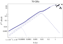
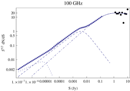
Figure 1: Fits of the hybrid model/data number counts for each frequency. The solid line is the empirical fit whereas the dots represent the De Zotti et al. model number counts (thin light dots) and Planck data (dark thick dots). The three curves under the fit are the three contributions (Low, Med and High, respectively dotted, dashed and dot-dahsed lines) which sum in the total fit. From top to bottom: $70$ GHz, $100$ GHz, $143$ GHz.

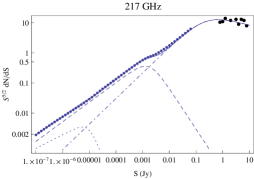
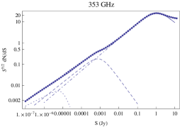
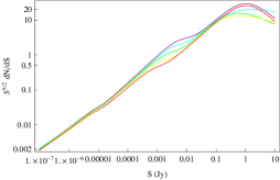
Figure 2: Fits of the hybrid model/data number counts for each frequency. The solid line is the empirical fit whereas the dots represent the De Zotti et al. model number counts (thin light dots) and Planck data (dark thick dots). The three curves under the fit are the three contributions (Low, Med and High, respectively dotted, dashed and dot-dahsed lines) which sum in the total fit. From top to bottom: $217$ GHz, $353$ GHz. Bottom is the comparison of the fits for the different frequencies: $70$ GHz is purple, $100$ GHz is cyan, $143$ GHz is green, $217$ GHz is yellow, $353$ GHz is orange.

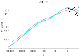
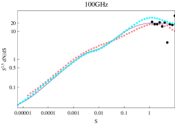
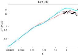
Figure 3: Comparison of the fits of the hybrid model/data number counts with the Tucci et al. model for each frequency. The solid line is the empirical fit whereas the cyan dots represent the De Zotti et al. model number counts (thin light dots) and Planck data (dark thick dots). The Tucci et al. model is represented by pink dots. From top to bottom: $70$ GHz, $100$ GHz, $143$ GHz.

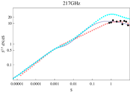
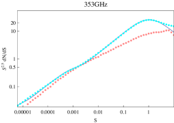
Figure 4: Comparison of the fits of the hybrid model/data number counts with the Tucci et al. model for each frequency. The solid line is the empirical fit whereas the cyan dots represent the De Zotti et al. model number counts (thin light dots) and Planck data (dark thick dots). The Tucci et al. model is represented by pink dots. From top to bottom: $217$ GHz, $353$ GHz.

In Figs. 3 and 4 we compare our hybrid number counts to those of (2011) based also on the ERCSC. Our fit overpredicts the number counts in the range $0.01-1$ Jy with respect to the Tucci et al. model. This overprediction is due to the fact that the flux density at we match the predictions and the data is 0.01 Jy whereas Tucci et al. chose a lower value.

Using the obtained composite counts we compute the Poissonnian power spectra at the considered frequencies. They are given by following expressions:

$$C_{\nu}^{\mathrm{R}adioPois} = \Sigma_{i=1,3}P_{i,\,\nu}S_{\mathrm{max},\,\nu}^{\chi_{i,\,\nu}}$$ (2.4)

$$\times 2F_{1}[a_{i,\,\nu},b_{i,\,\nu},c_{i,\,\nu},d_{i,\,\nu}S_{\mathrm{{max},\,\nu}}^{e_{i\,\nu}}(\nu)]$$

where $2F1$ are the Hypergeometric functions of second type (, 1965), the sum on $i$ is over the three contributions Low, Med and High, and the coefficients and exponents depend on the frequency and are reported in Table 6. The values of the Poissonian contribution to the angular power spectrum that we obtained from our fitted number counts are reported in the third column of Table 1. For comparison in the fourth column we report the values computed from the original De Zotti-model fits. As expected from the number counts comparison, we have a higher Poissonian contribution than the one obtained with the Tucci et al. model, namely 30% higher at 70 and 100 GHz, 40 and 60% at 143 and 217 GHz respectively. At 353 GHz we predict an amplitude twice larger.

Together with the term coming from the radio sources it is necessary to consider the Poissonian contribution of infrared galaxies which is relevant only for the higher frequency channels the 143, 217 and 353 GHZ. The values of the Poissonian infrared contributions at these frequencies are computed from the (2011) model in (2011b) and reported in the fifth column of Table 1. We summed the two Poisson terms for radio and infrared in the frequencies in a single Poissonian term:

$$C_{l,\nu}^{\mathrm{{PS,TOT}}}=A_{\mathrm{{PS}}}C_{l,\nu}^{\mathrm{{PS,Radio+IR}}}\,,$$ (2.5)

where $C_{l,\nu}^{\mathrm{{PS}}}$ is the Poissonian contribution at the different frequencies whereas $A_{\mathrm{{PS}}}$ which incorporates deviations of real data from this model remains the same for all the frequency considered.

$\rm{Channels}$	$S_{\rm max}$	$C_{\ell,{\rm Hybrid}}^{\rm Pois,Radio}$	$C_{\ell\,{\rm Original}}^{\rm Pois,Radio}$	$C_{\ell\,\mathrm{IR}}^{\rm Pois}$
	$\rm(J_{y})$	$\rm{(\mu K^{2})}$	$\rm{(\mu K^{2})}$	$\rm{(\mu K^{2})}$
$70$	$0.57$	$1.13\times 10^{-3}$	$1.08\times 10^{-3}$
$100$	$0.41$	$2.05\times 10^{-4}$	$2.25\times 10^{-4}$
$143$	$0.25$	$4.52\times 10^{-5}$	$4.86\times 10^{-5}$	$1.2\pm 0.2\times 10^{-5}$
$217$	$0.16$	$1.60\times 10^{-5}$	$1.74\times 10^{-5}$	$6\pm 1\times 10^{-5}$
$353$	$0.33$	$9.40\times 10^{-5}$	$1.03\times 10^{-4}$	$1.9\pm 0.3\times 10^{-3}$

Table 1: Poissonian contributions to the angular power spectrum for each frequency. In the first column are reported the observational frequencies and in the second the detection threshold fluxes. In the third column are reported the values of the Poissonian angular power spectrum for radio sources obtained using the composite number count fits. In the fourth column are reported the values of the Poissonian angular power spectrum computed using the original De Zotti et al. model number counts instead of the composite ones. In the last column are reported the values of the Poissonian term for infrared sources as predicted in (, 2011b).

2.4 Contribution from clustering term

The Cosmic Infrared Background (CIB) is the integrated IR emission over all redshifts of unresolved infrared star forming galaxies (, 2005). This contribution is mainly that of starbust galaxies, Luminous InfraRed Galaxies (LIRGs, $10^{11}L_{\odot}<L_{IR}<10^{12}L_{\odot}$) and Ultra Luminous InfraRed Galaxies (ULIRGs, $L_{IR}>10^{12}L_{\odot}$), (with small contribution from AGN) (, 2003, 2005, 2008). One of the complexity related to the CIB is that at different frequencies it accounts for contributions of IR sources from different redshift ranges (e.g. (2008)).

The clustering power spectrum is given by (2001, 2008, 2011):

$$C_{\ell}^{\rm Clust} = \int dz\frac{a^{2}(z)}{d_{A}^{2}}\frac{dr}{dz}\times$$ (2.6)

$$\bar{j}^{2}_{\lambda}(z)P_{g}(k)|_{k=\ell/d_{A}}(z)\,,$$

where $r$ is the proper distance, $d_{A}$ is the comoving angular diameter distance, $k=\ell/d_{A}$ derives from the Limber approximation, the $\frac{dz}{d_{A}^{2}}\frac{dr}{dz}a^{2}(z)$ term takes into account all geometrical effects and depends on the cosmological model adopted, $\bar{j}^{2}_{\lambda}(z)$ is the mean galaxy emissivity per unit of comoving volume and $P_{g}$ is the galaxy three-dimesional power spectrum . The emissivity of infrared galaxies can be written as (, 2011):

$$j_{\nu}(z)=\left(a\frac{d\chi}{dz}\right)^{-1}\int_{L}S(L_{IR})\frac{dN}{dzd(lnL_{IR})}d(ln{L_{I}R})$$ (2.7)

where $\frac{dN}{dzd(lnL_{IR})}$ is the luminosity function and $S$ is the flux. The clustering term as shown by Eq. 2.6 depends on the cosmological model through the geometrical factor, and through the galaxy power spectrum. Another complication is given by the indirect dependence of the emissitivity on the assumptions on the galaxy Spectral Energy Distribution (, 2001, 2008). Finally, the bias, relating the the emissivity fluctuations to the dark matter density fluctuations, also affects the clustering term and is poorly known. In view of the the theoretical complexity of the clustering term, we rather used the observational clustering term extracted directly from Planck maps at 217 and 353 GHz by (2011b). In order to minimally paramatrize this contribution, we have fitted the Planck best fit models. Since the Planck data are not available for the channels below 217 GHz, the values for the clustering term for 100 and 143 GHz channels were derived using the halo occupation distribution best-fit parameters of the 217 GHz channels (Table 7 of (2011b)), combined with the emissivities at 143 and 100 GHz computed using the (2011) model.

The fit to the clustering term is given for all the frequencies by the following expression:

$$\ell(\ell+1)\frac{C_{\ell}^{\rm clust}}{2\pi}(\nu)\propto\Big{(}\phi(\ell,\nu)+\beta(\nu)\frac{\log(\ell)^{\alpha(\nu)}}{(100+\ell)^{\gamma(\nu)}}\Big{)}\,,$$ (2.8)

where $\phi(\ell,\nu)$ is a fifth order polynomial term $A_{0}/\ell^{2}+A_{1}/\ell+A_{2}+A_{3}\ell+A_{4}\ell^{2}+A_{5}\ell^{3}+A_{6}\ell^{4}$ accounting for the steepening at high $\ell$, whereas the low $\ell$ shape is dominated by a complex logarithmic form. The coefficients $A_{0-6}$ depend on the frequency. The first step to obtain a fit to the clustered term was derive a spectral shape, namely the combination of a polynomial component with the logarithm form. Then we fitted the form given in Eq. 2.8 for each frequency first fitting the logarithmic function and then the polynomial function. Finally, we have derived the frequency dependence of each coefficient $A_{0-6}$ and each exponent by fitting to the different frequency. The resulting fit to the power spectrum is given by:

$$\ell(\ell+1)\frac{C_{\ell}^{\rm clust}}{2\pi} = \Sigma_{i=0,6}A_{i}\ell^{(i-2)}+A_{7}(\nu)\frac{\log(\ell)^{A_{8}(\nu)}}{(100+\ell)^{A_{9}(\nu)}}\,,$$

$$A_{i} = \Sigma_{j=1,3}a_{i}^{j}\nu^{j}\,,$$ (2.9)

where the first sum, on $i$, is on the coefficients of the polynomial and the second, in $j$ is on the polynomial dependence on the frequency. In Table 7 are reported the coefficients $a_{i}^{j}$. Such complex formula insures an accuracy of the fit at $<1\%$ level in all $\ell$ range, and at $<0.1\%$ in about $90\%$ of the considered $\ell$ range.

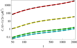
Figure 5: Comparison between the best fit models from data (for 217 and 353) and extrapolations (for 100 and 143) of the infrared source clustering (dashed) and the fits (solid line) for the various frequency channels. Colors: Cyan $100$ GHz, Green $143$ GHz, Yellow $217$ GHz, Red $353$ GHz.

Finally, provided the expression Eq. 2.9 giving the frequency-dependent CIB clustering power spectrum, the parametrization of the clustering term can be simply written as:

$$C_{\ell}^{\rm clust}(\nu)=A_{\rm CL}C_{\ell}^{\rm clust}(\nu)$$

where the amplitude parameter $A_{\mathrm{CL}}$ accounts for deviations of the real signal from our parametrisation.

3 Methodology

In the previous section we have detailed how we construct a frequency dependent parametrization for the point sources and TSZ contributions to the angular power spectrum. In Fig. 6 we display each contribution together with the primary CMB spectrum for the five frequencies of interest. As anticipated, we note that the higher frequency channels are dominated by the clustering term contribution, the $353$ GHz channel being the most contaminated. The lower frequencies are in turn dominated by the Poissonian term contribution. We also note that at small scales the TSZ contribution remains subdominant with respect to that of the point sources. As seen in Fig. 6, displaying the comparison between the sum of all contributions with the primary CMB, the $353$ GHz channel is the most contaminated due to the clustering contribution, whereas the cleanest channel is the $143$ GHz due to the low contribution of both clustering and Poissonian terms. We show in Table 2 the relative importance of the two main contributions of clustering and Poissonian expresssed in terms of the root mean square:

$$\sigma=\sqrt{\Sigma_{l}(2l+1)b_{l}^{2}C_{l}/(4\pi)}\,.$$ (3.11)

We note again how the high frequencies have a dominant clustering contribution whereas for the 100 and 143 GHz the dominant contribution is the Poissonian term.

$\rm{Channels}$	$\sigma^{\rm Clustering}$	$\sigma^{\rm Pois,Radio}$	$\sigma^{\rm Pois,IR}$
	$Jy/\sqrt{sr}$	$Jy/\sqrt{sr}$	$Jy/\sqrt{sr}$
$100$	$193.906$	$789.309$
$143$	$427.572$	$786.607$	$405.302$
$217$	$2890.06$	$873.219$	$1690.98$
$353$	$14927.1$	$1312.22$	$5899.56$

Table 2: Rms of the different contributions compared. In the first column are reported the interested frequencies. In the second column are reported the values of the clustering rms, in the third the Poissonian rms for radio sources and in the fourth the rms values for the Infrared Poissonian.

Since we are interested in small scale anisotropies it is possible to avoid the component separation process to remove diffuse emission from our galaxy and use instead single frequency angular power spectra derived by masking the Galaxy and the resolved point sources. The Galaxy may contribute even after masking with high latitude emissions and residuals which may remain depending on the aggressiveness of the mask used. In this work, we neglect the possible residuals, after masking, from Galactic contamination.

We combine the angular power spectra of the microwave sky at the considered frequency channels in a single power spectrum that we use to estimate the cosmological parameters. An optimal method to combine channels is the inverse noise variance weighting scheme (, 2009). This weighting scheme indeed gives the larger weights to the channels with higher resolutions and lower noise levels. This scheme is particularly adapted to the case of high multipole analysis where the noise and the beam smearing start to dominate. We therefore use a weighted linear sum of single frequency power spectra:

$$C_{\ell}^{\mathrm{tot}}=\Sigma_{i}w_{i}(\ell)C_{\ell}^{i}$$

where the summation in $i$ is over the frequencies.

For simplicity, the noise is modelled as an isotropic Gaussian white noise with variance $\sigma_{N}^{2}$ on the total integration time. We define the beam function as:

$$b^{2}_{\ell}=e^{-\ell(\ell+1)(0.425\,\mathrm{FWHM}/60\,\pi/180)^{2}};$$ (3.12)

where FWHM is the full width half maximum of the channel-beams in arcminutes. We illustrate our method on a Planck-like case taking the beams and noise characteristics from (2011),(2011). Moreover, the noise has been divided by $2$ to account for the approved extension of the mission. The numbers are summarised in Table 3.

We can thus define the noise function as:

$$N_{\ell}=\frac{(\sigma_{N})^{2}\Omega_{\mathrm{pix}}}{b^{2}_{\ell}}\,,$$ (3.13)

where $\Omega_{\mathrm{pix}}$ is the area corresponding to the pixel. Note that the total noise contribution to the angular power spectrum considers also the contribution of the observed sky fraction $\Delta C_{l}/Cl=N_{\ell}\sqrt{2/(f_{sky}(2\ell+1))}$. Assuming that the sky fraction in the different channels is the same, the contribution of this term cancels in the weights. With these definitions the weights for the single frequency spectrum is given by:

$$w_{i}(\ell)=\frac{\frac{1}{N^{2}_{\ell_{i}}}}{\Sigma_{j}\frac{1}{N^{2}_{\ell_{j}}}}\,,$$ (3.14)

where $i$ stands for the specific channel whereas $j$ runs over all channels.

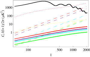
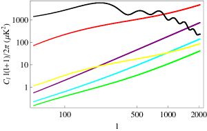
Figure 6: Comparison of the extragalactic signals with primary CMB (black solid line) for the different frequencies. The line color represent the frequency: $70$ GHz (purple), $100$ GHz (cyan), $143$ GHz (green), $217$ GHz (yellow), $353$ GHz (red). In the upper panel we show the comparison for each frequency of the three extragalactic signals: dotted is the clustering term, dashed is the Poissonian term and solid is TSZ. In the lower panel we show the comparison of the total astrophysical contribution with the CMB for each frequency. The solid lines are the sum of the TSZ, Poissonian and clustering contribution and follow the color scheme above.

Instrument	LFI	HFI
Center frequency GHz	70	100	143	217	353
Mean FWHM (arcmin)	13	9.88	7.18	4.71	4.5
$\Delta T$ per pixel ($I$)	24.2525	8.175	5.995	13.08	54.5
$\Delta T$ per pixel ($Q\,\&U$)	34.6075	13.08	11.1725	24.525	103.55

Table 3: Planck channel performance characteristics (, 2011, 2011) for the nominal mission.

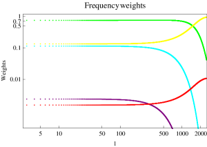
Figure 7: Weights of the different frequencies with the inverse noise variance scheme: purple $70$ GHz, cyan $100$ GHz, green $143$ GHz, yellow $217$ GHz, red $353$ GHz.

We show the weights obtained using the inverse noise variance scheme in Fig. 7. We note how the dominant contribution among the various combinations is given by the $143$GHz and $217$ GHz channels which have higher resolution and lower noise level, whereas channels with lower angular resolution have very little weights like the $70$ GHz whose contribution is strongly subdominant within this approach.

4 Estimating the cosmological and extragalactic parameters

We now show the results of our analysis where we have applied, to the mock data, our approach of frequency-dependent minimal parametrisation of the extragalactic sources. We first show the capability of our approach to perfectly recover the input cosmological parameters in presence of extragalactic contamination and exhibit the importance of the wide frequency range for the characterization of the extragalactic signals by comparing the results for different frequency combinations. Then we show the impact of the astrophysical contributions to the power spectrum and to the cosmological parameters and their errors. We finally test the robustness of our approach by investigating the dependence of the results on the astrophysical models we used. We will show also the results in the extended parameter space in particular we considered the case of a $\Lambda$CDM with running of the spectral index and tensor modes.

We developed an extension of the publicly available CosmoMC code (, 2002) which, in addition to estimating the cosmological parameters, estimates at the same time the contributions of a Poissonian term, a clustering term and a TSZ term. This is done by deriving a minimal number of amplitude terms, namely $A_{\mathrm{SZ}}\,,A_{\mathrm{PS}}\,,A_{\mathrm{CL}}$, which represent the departures from the input point source and TSZ models.

In practice, we have modified the CAMB code (, 2000), version May 2010, to compute for each given frequency channel the sum of point-source and TSZ spectra as provided by our parametrization (Sect. 2) and the standard CMB angular power spectrum. The resulting total power spectra at the different frequencies are then combined in a single effective power spectrum in the CosmoMC code.

We first explore the frequency combination and its effect on the recovery of the cosmological and the astrophysical parameters. The latter are represented by the amplitudes $A_{\mathrm{SZ}}$, $A_{\mathrm{PS}}$ and $A_{\mathrm{CL}}$. We have considered the results using five combinations of frequencies: 143 and 217 GHz, 100 to 217 GHz, 100 to 353 GHz, 70 to 217 GHz, and finally all the frequencies under consideration 70 to 353 GHz, with a sky coverage of $f_{\mathrm{sky}}=0.85$. In order to establish which frequency combination recovers the cosmological and astrophysical parameters best, we have performed for each combination an MCMC analysis of mock data using a $\Lambda$CDM-based CMB plus the astrophysical contributions. For the latter we used the “nominal” contributions, which means all the amplitude terms were set to one ($A_{\mathrm{SZ}}=A_{\mathrm{PS}}=A_{\mathrm{CL}}=1$). All the channel combinations perfectly recover the cosmological parameters. The major differences are in the recovery of the astrophysical parameters, $A_{\mathrm{SZ}}$, $A_{\mathrm{PS}}$ and $A_{\mathrm{CL}}$, see Fig. 8. More specifically, the simplest combination of the 143 and 217 GHz channels recovers the Poissonian term with the smallest errors but it gives large errors for the clustering term. By contrast, the combination of all considered channels, 70 to 353 GHz, gives the largest errors for the Poissonian term but significantly reduces the errors on the clustering term. The clustering term being the most uncertain with respect to the Poissonian one, we chose to use the combination of the five channels in order to improve the constraints on this major contribution to the microwave sky at small angular scales.

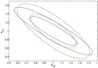
Figure 8: Comparison of the results for the two main astrophysical parameters of the analysis obtained with different frequencies, always combined with the inverse noise variance scheme: black (solid) is 70-353 GHz, red (short dashed) is 143-217 GHz, green (long dashed) is 100-217 GHz, blue (double dot dashed) is 70-217 GHz and the pink (dotted) line is the 100-353 GHz.

4.1 Standard $\Lambda$CDM model

We performed the analysis in the framework of a standard $\Lambda$CDM cosmological model. The input mock $C_{\ell}$ were produced with nominal values for the point source and TSZ contributions, namely $A_{SZ}=A_{PS}=A_{CL}=1$. Two cases are compared: Fixed values for the astrophysical parameters (fixed to one), and free values for $A_{\rm SZ}$, $A_{\rm PS}$, and $A_{\rm CL}$. The results are displayed in Fig. 9 and summarised in Table 4 (second column is the case with astrophysical parameters fixed to one, the third column is the case with astrophysical parameters variation), together with the input parameters (fourth column) . We show that the input cosmological parameters are accurately recovered in both cases. When the astrophysical parameters $A_{\rm SZ}$, $A_{\rm PS}$, and $A_{\rm CL}$ together with the cosmological parameters are let free the errors bars are slightly enlarged. The astrophysical parameters, $A_{\mathrm{PS}}$ and $A_{\mathrm{CL}}$, which characterize the point sources (Poissonian and clustering terms) are recovered well but they exhibit a strong degeneracy. This degeneracy is expected, in fact the Poissonian and the clustering terms have different shapes but they both contribute additively to increase the measured power at high multipoles. The results are the same when we use the Tucci et al. model rather than out hybrid model for the radio contribution. The amplitude of TSZ spectrum in turn remains unconstrained due to its subdominance with respect to the other two contributions of point sources. We will thus not discuss it further.

We now explore the robustness of the approach, in terms of parameter recovery, with respect to the models we use for the point source contributions. We do not vary the TSZ signal as it is subdominant and cannot be recovered. For the effects of TSZ on the cosmological parameters in absence of point sources, we refer the reader to (2008, 2009). We generated mock data including the CMB, the nominal TSZ contribution and the point source contributions (Poisson and clustering terms). The later have been chosen to differ significantly from the nominal contributions.

We first focus on the Poissonian term and multiplied the nominal Poissonian term by two in the mock data for each frequency channel leaving untouched the other contributions. In Fig. 10 we present the obtained cosmological and astrophysical parameters. It is worth noting that even with a much larger Poissonian contribution the cosmological and the astrophysical parameters, $A_{\mathrm{PS}}$ and $A_{\mathrm{CL}}$, are perfectly recovered.

Parameter	Best Fit value I	Best fit value II	Input value
$\Omega_{b}h^{2}$	$0.02251\pm 0.0001$	$0.02254\pm 0.0001$	$0.0225$
$\Omega_{c}h^{2}$	$0.1121\pm 0.001$	$0.1122\pm 0.001$	$0.112$
$\tau$	$0.0885\pm 0.004$	$0.0874\pm 0.004$	$0.088$
$n_{s}$	$0.967\pm 0.003$	$0.966\pm 0.004$	$0.967$
$\log[A_{s}10^{10}]$	$3.19\pm 0.007$	$3.19\pm 0.007$	$3.19$
$H_{0}$	$69.96\pm 0.5$	$69.94\pm 0.54$	$70$
$A_{PS}$	$-$	$0.99\pm 0.17$	$1$
$A_{CL}$	$-$	$1.01\pm 0.22$	$1$
$A_{SZ}$	$-$	$-$	$1$

Table 4: Comparison between the resulting best fit and the input values for the cosmological and extragalactic parameters. The fiducial model for the mock data is reported in the fourth column. In the second column are given the parameters recovered when taking into account the nominal contributions of the point sources and TSZ signals (note that the $A_{SZ}$ remains unconstrained). In the third column the parameters recovered when varying also the parameters of the contributions of the point sources and TSZ signals. The CMB plus extragalactic contribution power spectrum obtained using the best fit values and the one generated using the fiducial model values do not differ by more than 0.2%.

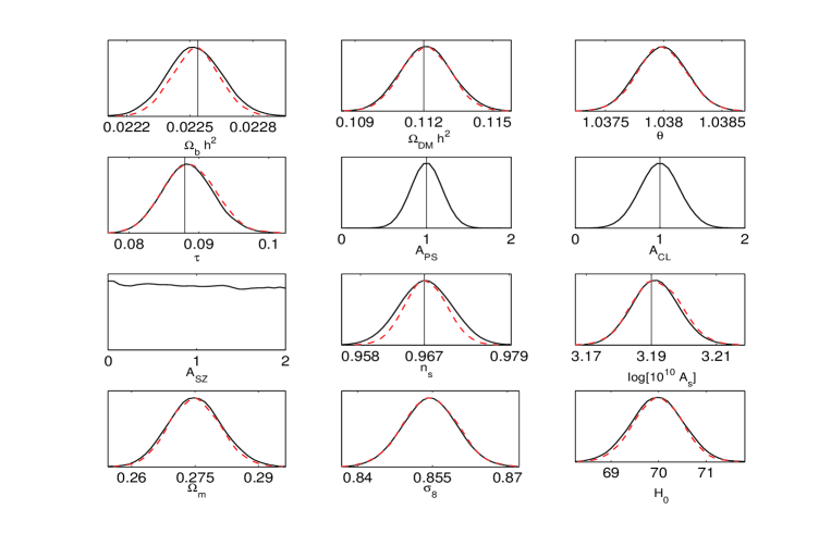
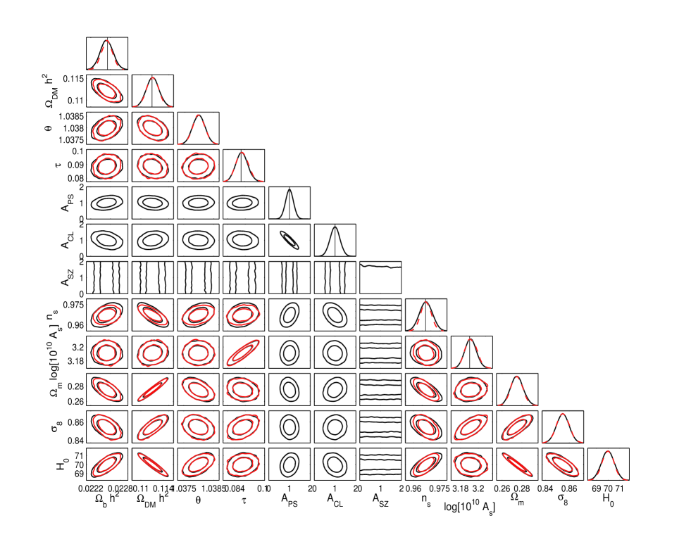
Figure 9: Cosmological (and astrophysical) parameters with and without varying the astrophysical contribution parameters. The five frequency channels are combined with the inverse noise variance weighting scheme. The black (solid) curve represents the analysis which in addition to cosmological parameters varies also the astrophysical ones whereas the red (dashed) curve represents the analysis with astrophysical parameters fixed to the fiducial model values. In the lower panel we show also the triangle plot which is useful to evidence possible degenerations. The curves are the $68\%$ and $95\%$ confidence level.

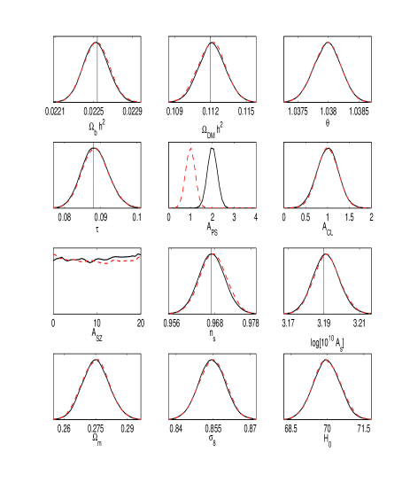
Figure 10: Robustness test part 1. Cosmological and astrophysical parameters with different astrophysical signals with respect to the fiducial model. The black (solid) curve are the results of the analysis which considers a Poissonian term which is two times its fiducial value. The red (dashed) curve represent the analysis with a clustering term for the 100 and 143 GHz doubled with respect to the fiducial value.

If we now focus on the clustering term, many tests with respect to the nominal model can be envisaged to test the effect of the parametrisation on the parameter recovery. We test the robustness of the results, or in other words the sensitivity to the clustering term, with respect to the frequency dependence of the clustering term by varying not only the amplitude but also the frequency dependence of the clustering term. The clustering term at 353 GHz being very well constrained by the present Planck measurements of the CIB, we choose not to vary it. The CIB measurements at 217 GHz by Planck, in turn, have larger errors (see (2011b)) and the values adopted in the parametrisation for the 100 and 143 GHz channels are empirical extrapolation based on the 217 GHz measure. Therefore it is very likely that at these frequencies the clustering term may be significantly different from what we used in the model. For this reason, we chose to vary these three frequencies.

We first analyse a case where we multiply by two the clustering contribution of the 100 GHz and 143 GHz channels. In Fig. 10 the results show that this modification does not affect significantly the cosmological nor the astrophysical parameters. The reason is that at 100 and 143 GHz the clustering term is not the dominant astrophysical component and therefore in the frequency combined spectrum the variation of the clustering term for these two frequencies does not modify the final result. In the inverse noise variance weighting combination scheme the major contribution to the clustering term comes from the 217 GHz channel which has a strong clustering component and at the same time is the dominant channel at high multipoles in the frequency combination. Since the 217 GHz measurements of the clustering still allow a rather significant variation, we decided to test the effects of a variation of the 217 clustering contribution by varying it by a factor 2. The obtained contribution differs by several sigmas from the present constraints obtained by Planck. We see from Fig. 11 that the cosmological parameters are perfectly recovered either when we multiply or when we divide the 217 GHz clustering contribution by two. Unsurprisingly, the recovered mean values of $A_{\rm CL}$ are multiplied/divided by a factor near two following to the varied contribution. Due to the degeneracy between the Poissonian and clustering terms, the mean values of $A_{\rm PS}$ are also shifted with respect to the input value.

We now test the robustness of the cosmological parameter recovery with respect to the frequency dependence that we proposed in our parametrisation of the clustering term. To do so, we multiply by two the clustering terms of the 100 and 143 GHz, whereas the clustering term at 217 GHz is multiplied and then divided by two. Here again the cosmological parameters are perfectly recovered in both cases whereas the amplitudes of the Poisson and clustering terms vary. The results obtained for the mean values of $A_{\rm PS}$ and $A_{\rm CL}$ are the same as those resulting from varying only the 217 GHz contribution. This comes from the dominance of the 217 GHz channel weight, in the channel combination, which in turn imply a dominance of the clustering term in the analysis.

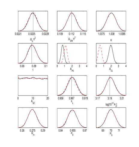
Figure 11: Robustness test part 2. Cosmological and astrophysical parameters with different astrophysical signals with respect to the fiducial model. The black (solid) curve are the results of the analysis which considers the 217 GHz clustering term double its fiducial value. The red (dashed) curve represent the analysis with a clustering term for the 217 GHz half its fiducial value.

We also tested the case where the Poissonian contribution is completely different from our model. To do so, we analyse the data using our hybrid model whereas we construct the mock data from the Tucci et al. model. By doing so, the Poissonian term varies from frequency to frequency whereas the IR contribution is the same as in the previous tests. In Fig.12 we show that this different Poissonian contribution does not alter the cosmological parameters but the astrophysical ones are modified. In particular the Poissonian contribution moves along the degeneracy line and the clustering amplitude is shifted.

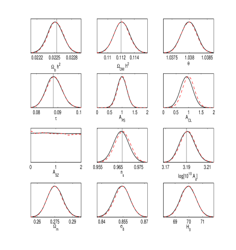
Figure 12: Comparison of the cosmological and astrophysical parameters obtained with the analysis which considers the standard De Zotti et al. based radio Poissonian (red curve) and the one which considers the Tucci et al. based radio Poissonian in the mock data and the standard De Zotti et al. based Poissonian in the code (black curve).

4.2 Extended cosmological parameter space

We have shown the results of the cosmological and astrophysical parameter recovery for a standard Lambda six-parameter cosmological model. We now present some results obtained in the case of an extended cosmological parameter space.

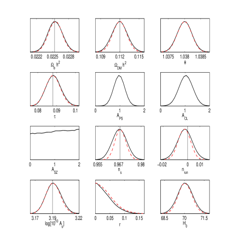
Figure 13: Results of the analysis which considers together with cosmological and astrophysical parameters also the variation of the tensor to scalar ratio and the running of the spectral index. Comparison between the results varying or not the astrophysical contributions: the black (solid) curve considers the astrophysical signals whereas the red (dashed) curve represent the results with astrophysical contributions fixed to the fiducial value. Vertical bars are the input parameters.

We considered together with the six standard parameters both tensor perturbations and the running of the spectral index, varying the tensor-to-scalar ratio, $r$, and the running, $n_{\rm run}$, together with the six standard parameters and the three astrophysical ones. We have generated the mock data with both extra parameters, $n_{\rm run}$ and $r$ set to zero. We fix the tensor spectral index to the second order inflationary consistency condition $n_{\mathrm{T}}=-\frac{A_{\mathrm{s}}}{8}\left(2-\frac{A_{\mathrm{s}}}{8}-n_{\mathrm{s}}\right)$. We included only the TE and EE mode in polarization we do not include the $B$-mode polarization power spectra in the exact form of the CMB likelihood we exploit, since the main limitation in that respect is given by the ability of removing diffuse foregrounds rather than instrumental noise. In Fig. 13 we show the comparison of the analyses which include the variation of the tensor-to-scalar ratio and the running of the spectral index, with fixed amplitudes of the point source contributions (red, dashed, curve) and without fixing the amplitudes of the point source contributions (black, solid, curves).

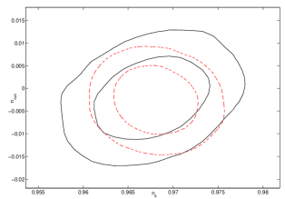
Figure 14: Results of the analysis which considers together with cosmological and astrophysical parameters also the variation of the tensor to scalar ratio and the running of the spectral index. Comparison between the results varying or not the astrophysical contributions: the black (solid) curve considers the astrophysical signals whereas the red (dashed) curve represent the results with astrophysical contributions fixed to the fiducial value. We show the comparison of the two analysis for the running of the spectral index and the scalar spectral index. Curves are the $68\%$ and $95\%$ confidence level.

Similarly to the standard $\Lambda$CDM model, leaving the astrophysical contributions free enlarges the errors bars including those of the running of the spectral index. The bi-dimensional plot of the scalar spectral index versus its running in Fig. 14 shows, in addition to the enlargement of the errors, a degeneracy between the two cosmological parameters. The combined variation of the tensor-to-scalar ratio and running, without the inclusion of $B$-mode polarization shifts the mean of the running of the spectral index towards negative values with respect to input ones ($n_{run}=0$).

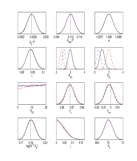
Figure 15: Robustness test part 4. Cosmological and astrophysical parameters with different astrophysical signals with respect to the fiducial model considering also the tensor perturbations and the running of the spectral index. The black (solid) curve are the results of the analysis which considers a Poissonian contribution double its fiducial value. The red (dashed) curve are the results of the analysis which considers the 100, 143 and 217 GHz clustering terms double their fiducial value. The blue (dot-dashed) curve represent the analysis with a clustering term for the 217 GHz half its fiducial value whereas double its fiducial value for 100 and 143 GHz.

We repeated also the main robustness analysis in this extended parameter space. In particular we repeated the three main cases: the case with the Poissonian contribution multiplied by two, the variation of both amplitude and frequency dependence of the clustering term with the multiplication by two of the 100 and 143 and multiplying and dividing by two the 217 term. In Fig.15 we report the results of the analysis. We note how the recovery of the parameters is the same as in the standard astrophysical case showing how our method is robust also for this extended parameter space.

5 Discussion and conclusions

In the present study, we developed a multi-frequency approach of the analysis of the CMB power spectrum aiming at obtaining unbiased cosmological parameters in the presence of unresolved extragalactic point sources and TSZ signal.

We have considered the three main extra-galactic contributions to the CMB signal at small scales, such as radio sources, infrared sources and SZ clusters. We have modelled these three signals in a minimal way using the observational constraints from Planck’s early results (, 2011a, b). In particular, the radio and IR sources were modelled through a unique Poissonian term and a unique clustering term. In total, three amplitude terms suffice to account for and characterize the extra-galactic contributions. This minimal number of parameters was obtained by considering the frequency dependences within our parametrizations of the TSZ signal, and IR and radio point sources.

The use of a data-based physical model including the frequency dependence of the astrophysical signals under consideration to build the parametrizations of the small-scale contribution to the CMB is one of the original points of the present work. Previous studies (, 2009, 2011) chose blind parametrizations of the signals which consider generic shapes and parametrize each frequency with a different set of parameters. Such an approach applied for a frequency channels, leads to either a rapid increase of the number of parameters necessary to describe the astrophysical signals, like in (2011), or it requires the use of a limited number of frequencies, like in (2009). Other studies focused only on one single contribution using more detailed and physical based parametrizations which involve a higher number of parameters with respect to our approach (see for example (2011) for the TSZ) or considered the frequency dependence on a much simpler level like for the clustering contribution in (2011). A different approach, relying directly on the data, has been used by the SPT team (, 2011, 2010). They took advantage of the high resolution to acquire data on scales where the CMB is suppressed. They used the data on smallest scales to measure the amplitudes of their blind templates for the astrophysical signals and consequently to remove the associated contamination from the CMB data.

We have applied our multi-frequency minimal parametrization of the extra-galactic contamination to estimate the cosmological parameters for a standard six-parameter $\Lambda$CDM model and for a model with tensor perturbations and a running of the spectral index, without including residuals from our Galaxy and without using the $B$-mode information. We show that the best combination of frequency is the one which considers the frequencies from 70 to 353 GHz. It allows to estimate the cosmological parameters and at the same to put the tightest constraints on the amplitude of the IR clustering term. We show, both in the standard $\Lambda$CDM model and in the ”extended-parameter” model, that the input cosmological parameters together with the astrophysical ones (amplitudes of the TSZ, Poisson and clustering terms) are recovered as unbiased and with slighlty enlarged error bars. We show that the Poisson and clustering terms are degenerate.

Our approach instead of blind parametrizations prefers to use the whole available information on point sources and theoretical knowledge of the TSZ to have models of the astrophysical signals which are the most similar as possible to the expected signal. The use of the frequency dependence and the technique used to fit the data allowed a very restricted number of parameters to characterize the signals, in particular only a total of three parameters for all the signals.

We have investigated for both cosmological models, standard and extended, the dependence of our approach and of the derived parameters on the accuracy of our model of extra-galactic contributions. In this way we tested its robustness against our theoretical priors on frequency dependence. We tested different Poissonian and clustering contributions by varying the associated terms both in amplitude and in frequency dependence. We showed that for both cosmological models the cosmological parameters are recovered unbiased even in situations where the mock data differ by several sigmas from the model. The astrophysical parameters, amplitudes $A_{\rm PS}$ and $A_{\rm CL}$, are recovered well in the case of a “real” Poissonian term different from that of the parametrisation. In the case of a different clustering term, the degeneracy with the Poissonian term induces a shift also in the Poissonian term.

We have provided a minimal parametrisation to take into account the extragalactic contaminations on small scales. Our minimal analysis can be extended to include additional contributions like residuals from the Galaxy contamination. However, it is ideal in the sense that systematic effects, beam uncertainties etc are not accounted for.

Channel	$70$	$100$	$143$	$217$	$353$
(GHz)
$A^{\mathrm{L}ow}$	8.06	7.76	7.47	7.16	6.81
$B^{\mathrm{L}ow}$	$10^{14}$	$10^{14}$	$10^{14}$	$10^{14}$	$10^{14}$
$C^{\mathrm{L}ow}$	1	1	1	1	1
$\alpha^{\mathrm{Low}}$	0.45	0.45	0.45	0.45	0.45
$\beta^{\mathrm{Low}}$	2.5	2.5	2.5	2.5	2.5
$w_{\nu}^{\mathrm{L}ow}$	4.4	4.0	5.0	7.5	4.5
$A^{\mathrm{Med}}$	306.98	224.99	241.08	203.69	165.85
$B^{\mathrm{Med}}$	20408	40000	111111	308642	501187
$C^{\mathrm{M}ed}$	1	1	1	1	1
$\alpha^{\mathrm{Med}}$	0.75	0.74	0.75	0.73	0.7
$\beta^{\mathrm{Med}}$	2.	2.	2.	2	1.9
$w_{\nu}^{\mathrm{M}ed}$	2.3	2.3	2.7	2.7	3.8
$A^{\mathrm{H}igh}$	58.41	22.66	70.89	23.12	51.17
$B^{\mathrm{H}igh}$	1.	0.91	3.52	1.48	0.93
$C^{\mathrm{H}igh}$	1	0.25	1	0.29	1
$\alpha^{\mathrm{H}igh}$	0.75	0.85	0.8	0.85	0.75
$\beta^{\mathrm{H}igh}$	1.45	1.0	1.2	1.1	1.5
$w_{\nu}^{\mathrm{H}igh}$	1.0	1.0	1.04	1.0	1.03

Table 5: The exponents $\alpha$, $\beta$ and the coefficients $A$, $B$, $C$ and $w_{\nu}$ for each term of the fits of the radio galaxies composite number counts.

Channel	$70$	$100$	$143$	$217$	$353$
(GHz)
$P_{1}$	$1.110^{-4}$	$3.6\times 10^{-5}$	$1.1\times 10^{-5}$	$4.3\times 10^{-6}$	$1.8\times 10^{-5}$
$\chi_{1}$	0.95	0.95	0.95	0.95	0.95
$a_{1}$	0.34	0.34	0.34
$b_{1}$	1	1	1	1	0.34
$c_{1}$	1.334	1.34	1.34	1.34	1
$d_{1}$	$-10^{14}$	$-10^{14}$	$-10^{14}$	$-10^{14}$	$-10^{14}$
$e_{1}$	2.5	2.8	2.8	2.8	2.8
$P_{2}$	$5.9\times 10^{-3}$	$1.4\times 10^{-3}$	$3.6\times 10^{-4}$	$1.5\times 10^{-4}$	$4.1\times 10^{-4}$
$\chi_{2}$	1.28	1.24	1.2	1.15	1.2
$a_{2}$	0.64	0.62	0.6	0.58	0.63
$b_{2}$	1	1.	1.	1.	1.
$c_{2}$	1.64	1.62	1.6	1.58	1.63
$d_{2}$	-20408.2	-40000	-111111.	-308642.	-501187
$e_{2}$	2	2	2	2	1.9
$P_{3}$	$2.6\times 10^{-3}$	$1.2\times 10^{-3}$	$3.6\times 10^{-4}$	$2.5\times 10^{-4}$	$4.5\times 10^{-4}$
$\chi_{3}$	1.25	1.35	1.3	1.35	1.25
$a_{3}$	0.86	1.	1	1.	0.83
$b_{3}$	1.	1.35	1.08	1.22727	1.
$c_{3}$	1.86	2.35	2.08	2.23	1.83
$d_{3}$	-1	-3.64	-3.52	-5.10	-0.93
$e_{3}$	1.45	1	1.2	1.1	1.47

Table 6: The coefficients and exponents of the radio galaxy Poissonian contribution to the angular power spectrum Eq.2.4.

$a_{i}^{j}$	j	0	1	2	3
i
0		14541.6	-298.31	1.84	$-3.26\times 10^{-3}$
1		-718.25	15.14	$-9.8\times 10^{-2}$	$1.9\times 10^{-4}$
2		19.52	- 0.42	$2.8\times 10^{-3}$	$-5.99\times 10^{-}6$
3		-0.19	$4.2\times 10^{-3}$	$-2.8\times 10^{-5}$	$6.1\times 10^{-8}$
4		$-2.\times 10^{-4}$	$4.4\times 10^{-6}$	$-3.03\times 10^{-8}$	$6.72\times 10^{-11}$
5		$1.83\times 10^{-8}$	$-3.99\times 10^{-10}$	$2.78\times 10^{-12}$	$6.18\times 10^{-15}$
6		$4.58\times 10^{-13}$	$-9.72\times 10^{-15}$	$6.50\times 10^{-17}$	$-1.36\times 10^{-19}$
7		-108.25	2.40	$-1.67\times 10^{-2}$	$3.66\times 10^{-5}$
8		3.81	$-6.03\times 10^{-2}$	$3.87\times 10^{-4}$	$-6.53\times 10^{-7}$
9		2.76	$-2.08\times 10^{-3}$	$-1.13\times 10^{-5}$	$4.07\times 10^{-8}$

Table 7: The coefficients and exponents of the fits for the clustering term Eq.2.9.

Acknowledgements: We wish to thank Nicolas Taburet for useful discussions and for providing the TSZ power spectrum template and Marco Tucci for provinding the number counts of (2011).This work is partially supported by ASI contract Planck-LFI activity of Phase E2, by LDAP. NA wishes to thank IASF Bologna for hosting and DP thanks IAS for hosting. The simulations for this work have been carried on IASF Bologna cluster. We wish thank the financial support by INFN IS PD51 for NA visit in Bologna.

References

- (1) Abramowitz M. and Stegun I., 1965, Handbook of mathematical functions with formulas, graphs, and mathematical table, New York: Dover Publishing
- (2) Addison G. E. et al., 2011, arXiv:1108.4614v1
- (3) Aghanim N, Majumdar S. and Silk J., 2008, Rept. Prog. Phys., 71,066902
- (4) Amblard A. et al., 2011, Nature, Volume:470, Pages: 510
- (5) Arnaud M., Pratt G.W., Piffaretti R., Boehringer H., Croston J.H., Pointecouteau E., 2009, arXiv:0910.1234v1
- (6) Ashby M. L. N. et al., 2009, ApJ, 701, 428-453
- (7) Bethermin M., Dole H., Lagache G., Le Borgne D. and Pénin A., 2010, arXiv:1010.1150v2
- (8) Danese L., Franceschini A., Toffolatti L. and de Zotti G, 1987, ApJL, 318, L15
- (9) Das S. et al., 2011, ApJ, 729, 62
- (10) De Zotti G., Burigana C., Negrello M., Tinti S., Ricci R., Silva L., González-Nuevo J., Toffolatti L., 2006, in The Many Scales in the Universe, JENAM 2004 Astrophysics Reviews, J.C. del Toro Iniesta et al. eds., Springer, Dordrecht, p. 45 astro, arXiv:astro-ph/0411182
- (11) De Zotti G., Ricci R., Mesa D., Silva L., Mazzotta P., Toffolatti L.,González-Nuevo J., 2005, A&A, 431, 893
- (12) Douspis M., Aghanim A. and Langer M., 2006, A&A, 456, 819d
- (13) Lagache G., Puget J.-L. and Dole H., 2005, ARA& A, 43
- (14) Dunkley J. et al., 2011, ApJ, 739, 52
- (15) Efstathiou G. and Gratton S., 2009, unpublished
- (16) Efstathiou G. and Migliaccio M., 2011, arXiv:1106.3208v1
- (17) Fernandez-Conde N., Lagache G., Puget J.-L. and Dole H.,2008, arXiv:0801.4299v1; 2010, arXiv:1004.0123v1
- (18) Gelman A. and Rubin D. B., 1992, Statistical Science, 7, 457
- (19) Hastings W. K., 1970, Biometrika, 57(1), 97
- (20) Keisler R. et al., 2011, arXiv:1105.3182v1
- (21) Knox L., Cooray A., Eisenstein D. and Haiman Z.,2001, ApJ, 550, 7-20
-
(22)
Komatsu E. et al., 2011, ApJS, 192, 18
- (23) Komatsu E. and Seljak U., 2002, MNRAS, 336, 1256
- (24) Lagache G., Dole H. and Puget J.-L., 2003, MNRAS, 338,555
- (25) Lewis A. and Bridle S.,2002, Phys. Rev. D, 66, 103511
- (26) camb Lewis A., Challinor A. and Lasenby A., 2000, ApJ, 538, 473
- (27) Lueker M. et al., 2010, ApJ, 719, 1045-1066
- (28) Marsden G.et al., 2009, ApJ, 707, 1729-1739; Ivison R.J. et al., 2010, MNRAS, 402, 245-258
- (29) Mennella A.et al., 2011, arXiv:1101.2038v4
- (30) Millea M., Doré O., Dudley J., Holder G., Knox L., Shaw L., Song Y.-S. and Zahn O., 2011, arXiv:1102.5195v1
- (31) Penin A., Doré O., Lagache G. and Bethermin M., 2011, arXiv:1110.0395v1
- (32) Planck Collaboration, 2006, Planck: The scientific programme,arXiv:astro-ph/0604069
- (33) Planck Collaboration, 2011a, Planck Early Results: Statistical properties of extragalactic radio sources in the Planck Early Release Compact Source Catalogue , arXiv:1101.2044
- (34) Planck Collaboration, 2011b, Planck Early Results XVIII: The power spectrum of cosmic infrared background anisotropies, arXiv:1101.2028
- (35) Planck HFI Core Team, 2011, Planck Early Results: The High Frequency Instrument data processing , arXiv:1101.2048v1
- (36) QUaD Collaboration, 2009, ApJ, 700, L187-L191
- (37) Redhead A. C. et al.,2004, ApJ, 609, 498-512
- (38) Reichardt C. L. et al., 2009, ApJ, 694:1200-1219
- (39) Sunyaev R. A. and Zeldovich Y. B.,1970, Astrophysics and Space Science, 7, 3; 1980, Annual review of astronomy and astrophysics, 18, 537
- (40) Sunyaev R. A. and Zeldovich Y. B., 1972, Comment Astrop. and Space Phys., 4, 173
- (41) Taburet N., Aghanim N., Douspis M. and Langer M., 2008, MNRAS, 392, 1153-1158
- (42) Taburet N., Aghanim N. and Douspis M., 2009, arXiv:0908.1653v1
- (43) Tinker J. L., Kravtsov A. V., Klypin A., Abazajian K., Warren M., Yepes G., Gottlöber S. and Holz. D. E., 2008, ApJ, 688, 709-728
- (44) Toffolatti L., Argueso Gomez F., De Zotti G., Mazzei P., Franceschini A., Danese L. and Burigana C., 1998, MNRAS, 297, 117-127
- (45) Toffolatti L., Negrello M., Gonzalez-Nuevo J., De Zotti G., Silva L., Granato G.L. and Argueso F., 2005, A&A, 438 475
- (46) Tucci M., Toffolatti L., De Zotti G., Martínez-González E., 2011, A&A, 533, A57
- (47) Tegmark M. and Efstathiou G., 1996, MNRAS, 281, 1297-1314