Tight Bell inequalities with no quantum violation from qubit unextendible product bases

Abstract

We investigate the relation between unextendible product bases (UPB) and Bell inequalities found recently in [R. Augusiak et al., Phys. Rev. Lett. 107, 070401 (2011)]. We first review the procedure introduced there that associates to any set of mutually orthogonal product vectors in a many-qubit Hilbert space a Bell inequality. We then show that if a set of mutually orthogonal product vectors can be completed to a full basis, then the associated Bell inequality is trivial, in the sense of not being violated by any nonsignalling correlations. This implies that the relevant Bell inequalities that arise from the construction all come from UPBs, which adds additional weight to the significance of UPBs for Bell inequalities. Then, we provide new examples of tight Bell inequalities with no quantum violation constructed from UPBs in this way. Finally, it is proven that the Bell inequalities with no quantum violation introduced recently in [M. Almeida et al., Phys. Rev. Lett. 104, 230404 (2010)] are tight for any odd number of parties.

I Introduction

It is well-established that quantum correlations (QC), i.e., correlations that can be obtained by local measurements on quantum states, offer applications with no classical analog. For instance, they provide cryptographic security not achievable by any classical cryptographic protocol Ekert ; bhk ; DIQKD , they enable the certification of the presence of randomness randomness ; colbeck , and, last but not least, outperform classical correlations (CC) at communication complexity tasks (see e.g. Ref. Commcompl ).

It is then interesting to ask whether quantum correlations are always more powerful than classical correlations. In other words, is it possible to find tasks at which classical correlations perform equally well as quantum? Such instances can be identified with the aid of Bell inequalities Bell , which are constraints satisfied by all CC. Any Bell inequality can be interpreted as the success probability of a task in which distant non-communicating parties are each given a certain input and then must compute, in a distributed manner, the correct value of a certain known function of the inputs. The violation of a Bell inequality by some correlations indicates that the corresponding task can be performed more efficiently by these correlations than by any CC. Consequently, correlations leading to a Bell violation do not have a classical realization. On the other hand, Bell inequalities with no quantum violation provide tasks at which QC offer no advantage over CC.

The first examples of Bell inequalities that cannot be violated by quantum theory were derived in Ref. Linden . These inequalities are nontrivial, as they are violated by non-signalling correlations, which, necessarily, do not have a quantum realization. The set of non-signalling correlations (NC) is defined to be the set of all those correlations which do not allow any instantaneous communication. However, the Bell inequalities found in Linden are not tight, which is an important feature in the present context (see Figure 1).

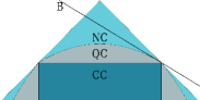
a)  b)

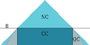
Figure 1: Schematic depiction of the sets of classical $CC$, quantum $QC$ and non-signalling correlations $NC$. Tight Bell inequalities correspond to facets of the classical set. $B$ denotes a Bell inequality with no quantum violation which is a) not tight, b) tight. Note that only tightness guarantees the existence of a non-trivial region in which quantum and classical correlations coincide.

Recall that a Bell inequality is called tight when it defines a facet of the convex set of CC (see e.g. Ref. polytopes ).

To our knowledge, the first nontrivial tight Bell inequalities which are not violated by quantum theory were those proposed in Ref. Mafalda . From a geometric point of view, the existence of such Bell inequalities implies that the convex sets of quantum and classical correlations can share facets. These inequalities were also used in a different context to prove that, contrary to the bipartite scenario Barnum ; Hadley , local quantum measurements and the no-signalling principle do not imply that correlations are quantum in a general multipartite scenario Hadley .

More recently, some of us have proposed a systematic construction of nontrivial Bell inequalities with no quantum violation my . The construction exploits the concept of unextendible product bases (UPBs) BennettUPB . This connection is remarkable, as UPBs are a notion of entanglement theory and heavily rely on the structure of tensor products of Hilbert spaces. Interestingly, this construction reproduces the Bell inequalities previously derived in Mafalda , thus proving that it may lead to tight Bell inequalities with no quantum violation. Unfortunately, these have so far been the only examples of tight Bell inequalities found via the construction. The main aim of this paper is to provide new examples of tight Bell inequalities with no quantum violation that arise from UPBs. To this end, we discuss in more detail how Bell inequalities can be derived from any set of mutually orthogonal product vectors in many-qubit Hilbert spaces and prove that the concept of unextendibility plays a crucial role for the nontriviality of the associated Bell inequality. In particular, we show that the only nontrivial Bell inequalities that can be constructed in this way are those coming from UPBs or sets that can be completed only to a UPB. We also prove that the Bell inequalities from Ref. Mafalda are tight for any odd number of parties.

This paper is structured as follows. Sec. II introduces all concepts relevant for the upcoming sections. In Sec. III, we recall the construction from my which associates to a set of mutually orthogonal product vectors a Bell inequality and study its properties in more detail. We prove that whenever the initial set of product vectors can be completed to a full basis of product vectors, then the resulting Bell inequality is trivial in the sense that it cannot be violated by any NC. In Sec. IV we show in more detail that the Bell inequalities from Mafalda can be constructed from UPBs and prove their tightness for any odd $n$. Sec. V presents new tight Bell inequalities with no quantum violation constructed from UPB, while Sec. VI concludes the paper.

II Preliminaries

Before getting to the results, let us first establish some terminology and notation and recall concepts and facts concerning unextendible product bases and nonsignalling correlations.

By abuse of terminology, we use the term “vector” in the context of quantum states always in the sense of “$1$-dimensional subspace of a complex Hilbert space”. Phrased differently, this means that we take our vectors to be unit vectors, and we identify two unit vectors whenever they differ only by a complex phase. By “basis”, we always mean an orthonormal basis.

II.1 Unextendible product bases

Consider a product $n$-partite Hilbert space

$$\mathcal{H}=\mathbbm{C}^{d_{1}}\otimes\ldots\otimes\mathbbm{C}^{d_{n}}$$ (1)

with $d_{i}$ $(i=1,\ldots,n)$ denoting local dimensions. Following Ref. BennettUPB , an unextendible product basis (UPB) is a collection of mutually orthogonal fully product vectors in $\mathcal{H}$,

$$U=\left\{|\phi^{(1)}_{j}\rangle\otimes\ldots\otimes|\phi^{(n)}_{j}\rangle\right\}_{j=1}^{|U|},$$ (2)

obeying two conditions: (i) $|U|<\mathrm{dim}\mathcal{H}=\Pi_{i=1}^{n}d_{i}$ ($U$ does not span $\mathcal{H}$), and (ii) $(\mathrm{span}\,U)^{\perp}$ does not contain any product vector, or, in other words, is a completely entangled subspace.

UPBs were introduced in the context of entanglement theory in Ref. BennettUPB , where they were used to obtain one of the first constructions of bound entangled states BennettUPB ; UPBhuge . More precisely, the state

$$\rho_{U}=\frac{\mathbbm{1}_{\mathcal{H}}-\Pi_{U}}{D-|U|}\,,$$ (3)

where $\Pi_{U}$ denotes the sum of projectors onto vectors from $U$, has positive partial transpose with respect to any bipartition, but nevertheless is entangled. While the former follows from the fact that the application of partial transposition with respect to any subset of parties to $\Pi_{U}$ returns another projector, the latter is a consequence of the lack of product vectors in $(\mathrm{span}\,U)^{\perp}$ and hence the range criterion applies here PHrange . UPBs are interesting and intriguing objects and hence there has been some effort towards understanding their properties and structure (see e.g. Refs BennettUPB ; UPBhuge ; upb ; Bravyi ).

To illustrate the above definition, let us provide two examples of UPBs.

Example 1.

First, we consider one of the earliest examples of a bipartite UPB, the so-called pyramid BennettUPB , $\mathcal{U}_{\mathrm{Pyr}}=\left\{|v_{j}\rangle\otimes|v_{2j\,\mathrm{mod}\,5}\rangle\right\}_{j=0}^{4}\subset\mathbbm{C}^{3}\otimes\mathbbm{C}^{3}$ with

$$|v_{j}\rangle=N\left(\cos\varphi_{j}|0\rangle+\sin\varphi_{j}|1\rangle+h|2\rangle\right),$$ (4)

where $N=2/\sqrt{5+\sqrt{5}}$, $h=(1/2)\sqrt{1+\sqrt{5}}$, and $\varphi_{j}=2\pi j/5$. One easily finds that there is no product vector in $(\mathrm{span}\,\mathcal{U}_{\mathrm{Pyr}})^{\perp}$ and hence $\mathcal{U}_{\mathrm{Pyr}}$ is a UPB in $\mathcal{H}=\mathbbm{C}^{3}\otimes\mathbbm{C}^{3}$. Let us also note that in the bipartite case, $\mathcal{U}_{\mathrm{Pyr}}$ is the lowest-dimensional example of a UPB: in $\mathbbm{C}^{2}\otimes\mathbbm{C}^{d}$ there are no UPBs for any $d$.

Example 2.

Let us now take the following four-element set of three-qubit vectors BennettUPB :

$$\mathcal{U}_{\mathrm{Shifts}}=\{|000\rangle,|1\overline{e}e\rangle,|e1\overline{e}\rangle,|\overline{e}e1\rangle\}$$ (5)

where $|e\rangle\in\mathbbm{C}^{2}$ is an arbitrary unit vector different from $|0\rangle$ and $|1\rangle$ and $|\overline{e}\rangle$ stands for the unit vector orthogonal to $|e\rangle$ (unique up to phase). This set is a slight generalization of the so-called “Shifts” UPB found in Ref. BennettUPB and then generalized to more parties in Ref. UPBhuge . Notice also that for each qubit, we can replace $\{|e\rangle,|\overline{e}\rangle\}$ with a different basis $\{|e_{i}\rangle,|\overline{e}_{i}\rangle\}$ $(i=1,2,3)$ independent of $|0\rangle$ and $|1\rangle$. Up to local unitary equivalence, there are no other UPBs in $\mathbbm{C}^{2}\otimes\mathbbm{C}^{2}\otimes\mathbbm{C}^{2}$ Bravyi .

II.2 Nonsignalling correlations

Let us consider $n$ observers having access to $n$ correlated systems. The $i$th observer $(i=1,\ldots,n)$ can perform on his system one of $m_{i}$ possible measurements with $r_{i}^{x_{i}}$ outcomes, henceforward denoted $a_{i}$, where $x_{i}\in\{0,\ldots,m_{i}-1\}$ stands for the measurement choice of the $i$th observer. The correlations established in this way are determined by the collection of conditional probabilities

$$\{p(\boldsymbol{a}|\boldsymbol{x})\equiv p(a_{1},\ldots,a_{n}|x_{1},\ldots,x_{n})\},$$ (6)

where $\boldsymbol{a}=(a_{1},\ldots,a_{n})$ and $\boldsymbol{x}=(x_{1},\ldots,x_{n})$. The usual way of dealing with these objects is to treat them as a vector in $\mathbbm{R}^{D}$ with $D=\prod_{i=1}^{n}\sum_{x_{i}=0}^{m_{i}-1}r_{i}^{x_{i}}.$

Clearly, the probabilities $p(\boldsymbol{a}|\boldsymbol{x})$ are nonnegative and normalized in the sense that $\sum_{\boldsymbol{a}}p(\boldsymbol{a}|\boldsymbol{x})=1$ holds for any $\boldsymbol{x}$. Additionally, as it is assumed that no communication among the parties can take place when the measurements are performed, the obtained correlations must obey the principle of no-signalling: the choices of observables by a set of parties cannot influence the statistics seen by the remaining parties. Formally, this can be stated as a set of equations of the form

$$\begin{split}&\sum_{a_{i}}p(a_{1}\ldots a_{i}\ldots a_{n}|x_{1}\ldots x_{i}\ldots x_{n})\\ =&\sum_{a_{i}}p(a_{1}\ldots a_{i}\ldots a_{n}|x_{1}\ldots x^{\prime}_{i}\ldots x_{n})\end{split}$$ (7)

for all $x_{i},x^{\prime}_{i}$, and $a_{1},\ldots,a_{i-1},a_{i+1},\ldots,a_{n}$ and $x_{1},\ldots,x_{i-1},x_{i+1},\ldots,x_{n}$ and all $i$. The conditional probabilities (6) constrained by the positivity, normalization and the nonsignalling conditions (7) form a polytope (see e.g. Ref. polytopes ) whose dimension depends on the considered scenario and is given by Lifting :

$$d=\prod_{i=1}^{n}\left[\sum_{x_{i}=0}^{m_{i}-1}(r_{i}^{x_{i}}-1)+1\right]-1.$$ (8)

Quantum correlations (QC).

Assume now that the parties have access to correlated quantum particles. The resulting correlations are then guaranteed to satisfy the no-signalling equations and read

$$p(a_{1},\ldots,a_{n}|x_{1},\ldots,x_{n})=\mathrm{Tr}\left[\varrho\,P_{x_{1}}^{a_{1}}\otimes\ldots\otimes P_{x_{n}}^{a_{n}}\right],$$ (9)

where $\varrho$ stands for a density matrix and $P_{x_{i}}^{a_{i}}$ denote positive operators representing the measurement outcomes at the $i$th site. For each $x_{i}$, they need to satisfy

$$\sum_{a_{i}}P_{x_{i}}^{a_{i}}=\mathbbm{1}\qquad(i=1,\ldots,n).$$ (10)

Since any quantum measurement can be realized as a projective measurement on a Hilbert space of sufficiently large dimension, we can always assume that all $P_{x_{i}}^{a_{i}}$ are orthogonal projectors.

Classical correlations.

Let us now consider correlations that can be established by the $n$ observers when they have access only to shared classical information in the form of shared randomness $\lambda$, which is a random variable with arbitrary distribution $p(\lambda)$. This defines the set of classical correlations (CC). It is the set of all those conditional probabilities which can be written in the form

$$p(\boldsymbol{a}|\boldsymbol{x})=\sum_{\lambda}p(\lambda)\prod_{i=1}^{n}p_{i}(a_{i}|x_{i},\lambda).$$ (11)

where each $p_{i}(a_{i}|x_{i},\lambda)$ is an arbitrary conditional probability distribution. It follows that, analogously to the case of NC, the set of all CC is a polytope in the same space. Its extremal points are the deterministic probabilities $p(\boldsymbol{a}|\boldsymbol{x})=\prod_{i=1}^{n}p_{i}(a_{i}|x_{i})$ where each probability $p_{i}(a_{i}|x_{i})$ equals either zero or one.

The set of CC is strictly smaller than the set of QC which Bell , in turn, is strictly smaller than the set of NC PR .

Bell inequalities.

Consider a linear combination of the conditional probabilities, $\sum_{\boldsymbol{a},\boldsymbol{x}}T_{\boldsymbol{a},\boldsymbol{x}}p(\boldsymbol{a}|\boldsymbol{x})$ with $T_{\boldsymbol{a},\boldsymbol{x}}$ being some $2n$-index tensor $T_{\boldsymbol{a},\boldsymbol{x}}$. Finding the maximal value, written as $\beta_{C}$, of this expression over all local probabilities (11), one arrives at the Bell inequality Bell :

$$\sum_{\boldsymbol{a},\boldsymbol{x}}T_{\boldsymbol{a},\boldsymbol{x}}p(\boldsymbol{a}|\boldsymbol{x})\leq\beta_{C}.$$ (12)

We say that a Bell inequality is nontrivial if it is violated by some NC, that is there exist NC, $p(\boldsymbol{a}|\boldsymbol{x})$, such that $\sum_{\boldsymbol{a},\boldsymbol{x}}T_{\boldsymbol{a},\boldsymbol{x}}p(\boldsymbol{a}|\boldsymbol{x})>\beta_{C}$.

Geometrically, nontrivial Bell inequalities are hyperplanes that separate CC from some NC, and possibly also from some QC. A Bell inequality is said to be tight whenever it defines a facet of the polytope of CC. Like any other polytope polytopes , the polytope of CC can be fully described in terms of its facets, that is by all the tight Bell inequalities. If some correlations do not have a classical realization, they necessarily violate a tight Bell inequality. This explains our interest in tightness.

Given a Bell inequality, how does one find out whether it is tight or not? It is tight if and only if those CC which saturate the Bell inequality span, when treated as vectors from $\mathbbm{R}^{D}$, an affine subspace of dimension $d-1$. So in order to check tightness, one has to see whether the models attaining the maximum value $\beta_{C}$ constitute a set of $d$ linearly independent vectors (for more detail see e.g. Refs. Lifting ; Lluis ).

Finally, let us mention that when rewritten in an appropriate form (entries of $T_{\boldsymbol{a},\boldsymbol{x}}$ are nonnegative and normalized), every Bell inequality can be understood as a nonlocal game as follows. Upon receiving, in a distributed manner, the input $\boldsymbol{x}$ (from some fixed set of possible inputs), the parties determine an output $\boldsymbol{a}$ and receive a payoff $T_{\boldsymbol{a},\boldsymbol{x}}$. Then, the left-hand side of (12) corresponds to the value of the game. Accordingly, the classical bound $\beta_{C}$ stands for the maximal value of the game in the case when the only resource at a disposal of the parties is a shared randomness. Then, violation of a Bell inequality by some QC means that there exist quantum resources allowing the parties to perform the corresponding task with greater efficiency than allowed by classical physics.

III Bell inequalities with no quantum violation from UPBs

In this section we recall and study in some more detail the scheme from Ref. my for constructing Bell inequalities from sets of orthogonal product vectors. Also, we prove that if the set of orthogonal product vectors can be completed to a full basis of product vectors (or already constitutes a full basis itself), then the associated Bell inequality is trivial in the sense that it cannot be violated by any NC.

III.1 The construction

We now restrict to an $n$-qubit Hilbert space $\mathcal{H}=({\hbox{\Bbb C}}^{2})^{\otimes n}$. Suppose that

$$\mathcal{S}=\left\{|\psi_{j}\rangle=|\psi_{j}^{(1)}\rangle\otimes\ldots\otimes|\psi_{j}^{(n)}\rangle\right\}_{j=1}^{|\mathcal{S}|},$$ (13)

is a set of product vectors in $\mathcal{H}$, where each $|\psi_{j}^{(i)}\rangle\in{\hbox{\Bbb C}}^{2}$ is a unit vector. In the following, we assume that the $|\psi_{j}\rangle$ are mutually orthogonal. This implies an upper bound on the number of elements of $\mathcal{S}$ given by $|\mathcal{S}|\leq 2^{n}$. For the time being, however, we do not assume $\mathcal{S}$ to be a UPB.

For each $i$, we now take the $|\psi^{(i)}_{j}\rangle$ to be ordered in such a way that the vectors in the local set

$$\mathcal{S}^{(i)}=\left\{|\psi^{(i)}_{1}\rangle,\ldots,|\psi^{(i)}_{s_{i}}\rangle\right\}$$

are all different, and such that each $|\psi^{(i)}_{j}\rangle$ for $j>s_{i}$ is already contained in this list. In general, either of $s_{i}<|\mathcal{S}|$ or $s_{i}=|\mathcal{S}|$ is possible.

Then we partition each $\mathcal{S}^{(i)}$ into disjoint subsets

$$\mathcal{S}^{(i)}=\mathcal{S}^{(i)}_{1}\cup\ldots\cup\mathcal{S}^{(i)}_{m_{i}}$$

such that two vectors in $\mathcal{S}^{(i)}$ are orthogonal if and only if they lie in the same subset of the partition. This is possible because of the following property of ${\hbox{\Bbb C}}^{2}$: if $|\phi^{\prime}\rangle$ is neither orthogonal to nor equal to $|\phi\rangle$, then it is also neither orthogonal to nor equal to $|\phi^{\perp}\rangle$. Alternatively speaking, orthogonality is an equivalence relation on vectors in ${\hbox{\Bbb C}}^{2}$.

In the framework of my , this has been called property (P), and it has also been noted that it is automatic in the qubit case. Since here we consider the qubit case only, each local subset $\mathcal{S}^{(i)}_{j}$ contains at most $2$ vectors. As example 1 shows, there exist sets of orthogonal product vectors without property (P) when the local Hilbert spaces have dimension higher than $2$.

Resuming the construction of the Bell inequality, we also need to fix an arbitrary ordering of each subset $\mathcal{S}^{(i)}_{j}$.

Now the Bell scenario associated to this $\mathcal{S}$ is given by $n$ parties, where party $i$ has $m_{i}$ measurement settings and every measurement has two possible outcomes.

The Bell inequality associated to $\mathcal{S}$ in this scenario is defined as follows. We assign to every product vector $|\psi_{j}\rangle\in\mathcal{S}$ a certain term $p(\boldsymbol{a}_{j}|\boldsymbol{x}_{j})$. This term is defined by a list of settings, $\boldsymbol{x}_{j}=(x_{j}^{(1)},\ldots,x_{j}^{(n)})$, and a list of outcomes, $\boldsymbol{a}_{j}=(a_{j}^{(1)},\ldots,a_{j}^{(n)})$. These are obtained through the procedure of

• determining the local vector $|\psi_{j}^{(i)}\rangle$ appearing at the $i$th site of $|\psi_{j}\rangle$ for each $i$,

• setting $x_{j}^{(i)}$ to be the number $k$ for which $|\psi_{j}^{(i)}\rangle\in\mathcal{S}_{k}^{(i)}$, while taking $a^{(i)}_{j}$ to be the position of $|\psi_{j}^{(i)}\rangle$ within $\mathcal{S}_{k}^{(i)}$.

Let us now take a linear combination of these terms, $\beta=\sum_{i}q_{i}p(\boldsymbol{a}_{i}|\boldsymbol{x}_{i})$, with nonnegative weights $q_{i}$, which always can be assumed to obey $0\leq q_{i}\leq 1$. This leads us to the Bell inequality

$$\sum_{i=1}^{|\mathcal{S}|}q_{i}p(\boldsymbol{a}_{i}|\boldsymbol{x}_{i})\leq\beta_{C},$$ (14)

where, as before, $\beta_{C}$ stands for the maximal value of the left-hand side of (14) over classical probability distributions (6).

Our main aim throughout the present paper is to investigate these inequalities, and, in particular, how their properties are related to the properties of the underlying sets $\mathcal{S}$. First, we prove that any such inequality cannot be violated by quantum theory. Denoting by $\beta_{Q}$ the maximal value achievable by the left-hand side of (14) within quantum theory, we have the following fact.

Theorem 1.

Let $\mathcal{S}$ be the set of mutually orthogonal vectors from $\mathcal{H}$. Then for the corresponding Bell inequality (14), $\beta_{C}=\beta_{Q}=\max\{q_{i}\}$.

Proof.

Orthogonality of any pair of vectors from $\mathcal{S}$ implies that at some position they have different vectors from the same local subset $\mathcal{S}^{(i)}_{k}$. This means that any pair of the associated conditional probabilities has at some site the same inputs but different outputs (different outcomes of the the same observable). Consequently, for any deterministic local model (recall that to get $\beta_{C}$ one can restrict to these models) if one of the conditional probabilities equals unity, the remaining ones vanish (let us call such probabilities “orthogonal”). Consequently $\beta_{C}=\max\{q_{i}\}$.

In order to prove that $\beta_{Q}=\max\{q_{i}\}$, we can always restrict to local von Neumann measurements and assign the product projectors

$$P_{j}=\bigotimes_{i=1}^{n}P_{j}^{(i)}$$ (15)

to the conditional probabilities $p(\boldsymbol{a}_{j}|\boldsymbol{x}_{j})$. Then, “orthogonality” of the conditional probabilities directly implies that $P_{j}\perp P_{k}$ for $j\neq k$. Consequently, the corresponding Bell operator

$$B=\sum_{j=1}^{|\mathcal{S}|}q_{j}\bigotimes_{i=1}^{n}P_{j}^{(i)}.$$ (16)

is a positive operator whose eigenvalues are the $q_{j}$’s, meaning that $\beta_{Q}=\max\{q_{j}\}$. This completes the proof. ∎

Corollary 2.

An immediate consequence of this fact is that for a given set $\mathcal{S}$, the strongest Bell inequality it generates (14) is the one with equal $q$’s. This is because the left-hand side of (14) can always be upper bounded by $\max\{q_{i}\}\sum_{j=1}^{|\mathcal{S}|}p(\boldsymbol{a}_{j}|\boldsymbol{x}_{j})$ and the latter expression give rise to a Bell inequality with the same classical bound as (14). Along the same lines, it is fairly easy to see that a Bell inequality with unequal $q$’s cannot be tight. Consequently, from now on we restrict to Bell inequalities with equal $q$’s, i.e. to

$$\sum_{i=1}^{|\mathcal{S}|}p(\boldsymbol{a}_{i}|\boldsymbol{x}_{i})\leq 1.$$ (17)

Let us illustrate the above construction by applying it to two particular sets of vectors.

Example 3.

First, consider the set $\mathcal{U}_{\mathrm{Shifts}}$ (5). Clearly, it has the property (P) and at each site we can distinguish two local sets $\mathcal{S}_{0}^{(i)}\equiv\mathcal{S}_{0}=\{|0\rangle,|1\rangle\}$ and $\mathcal{S}_{1}^{(i)}\equiv\mathcal{S}_{1}=\{|e\rangle,|\overline{e}\rangle\}$ $(i=1,2,3)$. Then, to each element of $\mathcal{U}_{\mathrm{Shifts}}$ we assign conditional probabilities in the following way: $|000\rangle\mapsto p(000|000)$, $|1\overline{e}e\rangle\mapsto p(110|011)$, $|e1\overline{e}\rangle\mapsto p(011|101)$, and $|\overline{e}e1\rangle\mapsto p(101|110)$. Summing up these probabilities we get the tight Bell inequality with no quantum violation found in Ref. Sliwa and studied in Ref. Mafalda :

$$p(000|000)+p(110|011)+p(101|110)+p(011|101)\leq 1.$$ (18)

Example 4.

Second, we take the full basis in the three-qubit Hilbert space $\mathcal{H}=(\mathbbm{C}^{2})^{\otimes 3}$ giving rise to the phenomenon called nonlocality without entanglement BennettNNWE :

$$\mathcal{S}=\{|000\rangle,|e01\rangle,|01e\rangle,|01\overline{e}\rangle,|1e0\rangle,|\overline{e}01\rangle,|1\overline{e}0\rangle,|111\rangle\}.$$ (19)

As before, we partition the set of local vectors into subsets; in this case, the local vectors are the same for each party, and the subsets are

$$\mathcal{S}_{0}=\left\{|0\rangle,|1\rangle\right\},\quad\mathcal{S}_{1}=\left\{|e\rangle,|\overline{e}\rangle\right\}.$$

Then, associating conditional probabilities to every element of $\mathcal{S}$ and following the above procedure, we arrive at the Bell inequality

$$p(000|000)+p(001|100)+p(010|001)+p(011|001)$$

$$+p(100|010)+p(101|100)+p(110|000)$$

$$+p(111|000)\leq 1.$$ (20)

This one, however, is trivial as it cannot be violated by any NC. Indeed, using nonsignalling conditions (7), it can be shown that the left-hand side of Eq. (4) is exactly one. This, as we will see shortly, is a consequence of the fact that $\mathcal{S}$ is a basis in $(\mathbbm{C}^{2})^{\otimes 3}$.

These two examples reflect the importance of the notion of UPB in our construction. Any set of product orthogonal vectors $\mathcal{S}\subseteq\mathcal{H}$ is either a UPB (or a set that can be completed only to a UPB), or completable to a full basis in $\mathcal{H}$ (or already one). In the second case, we will call the set completable. Interestingly, any Bell inequality constructed from the completable set is trivial in the sense that it cannot be violated by any NC. On the other hand, Bell inequalities associated to UPBs are always nontrivial as there exist NC violating them. The following two theorems formalize the above statements.

Theorem 3.

Let $\mathcal{S}$ be a set of orthogonal product vectors in an $n$-qubit Hilbert space $\mathcal{H}$. If $\mathcal{S}$ is completable, then the resulting Bell inequality (14) cannot be violated by any NC.

Proof.

Let us start by noting that any Bell inequality which is saturated by some interior point of the CC polytope is trivial. Then, the left-hand side of (12) has a constant value, equal to $\beta_{C}$, on the whole affine subspace spanned by all CC, and this subspace contains all nonsignalling correlations.

To see this more explicitly, assume that a given Bell inequality (12) is saturated by an interior point $\{\widetilde{p}(\boldsymbol{a}|\boldsymbol{x})\}$ of the corresponding CC polytope, i.e.,

$$\sum_{\boldsymbol{a},\boldsymbol{x}}T_{\boldsymbol{a},\boldsymbol{x}}\widetilde{p}(\boldsymbol{a}|\boldsymbol{x})=\beta_{C}.$$ (21)

We can always represent $\{\widetilde{p}(\boldsymbol{a}|\boldsymbol{x})\}$ as a convex combination of some extremal point (deterministic local point), denoted $\{p_{\mathrm{ex}}(\boldsymbol{a}|\boldsymbol{x})\}$, of this polytope and some other point lying on its boundary. This, when substituted into Eq. (21), directly implies that $\{p_{\mathrm{ex}}(\boldsymbol{a}|\boldsymbol{x})\}$ must saturate (12). Since any extremal point of the CC polytope can be used in this decomposition, (12) must be saturated by all of them. Consequently, any affine combination of the vertices of the CC polytope, and in particular any NC, also saturates (12).

Let us now assume that $\mathcal{S}$ is a full basis in an $n$-qubit Hilbert space $\mathcal{H}$ and consider the associated Bell inequality

$$\sum_{j=1}^{\mathrm{dim}\mathcal{H}}p(\boldsymbol{a}_{j}|\boldsymbol{x}_{j})\leq 1.$$ (22)

Then, let us take the uniform probability distribution, i.e., $p(\boldsymbol{a}|\boldsymbol{x})=1/\mathrm{dim}\mathcal{H}$ for any $\boldsymbol{a}$ and $\boldsymbol{x}$. On one hand, it clearly saturates the Bell inequality (22). On the other hand, it belongs to the interior of the corresponding CC polytope, which, in view of what we have just said, implies that (22) cannot be violated by any NC.

Finally, let us assume that $\mathcal{S}$ is not a full basis in $\mathcal{H}$, but can be completed to one. Let us write $\overline{\mathcal{S}}=\{|\phi_{j}\rangle\}_{j=1}^{\mathrm{dim}\mathcal{H}-|\mathcal{S}|}$ for the completing set of mutually orthogonal product vectors. Again $\mathcal{S}\cup\overline{\mathcal{S}}$ is a set of mutually orthogonal product vectors, and therefore has an associated Bell inequality

$$\sum_{j=1}^{\mathrm{dim}\mathcal{H}}p(\boldsymbol{a}_{j}|\boldsymbol{x}_{j})\leq 1.$$

In the previous paragraph, we showed that this inequality is trivial in the sense that all NC satisfy it with equality. Now we can upper bound the left-hand side of (17) for any NC $p(\boldsymbol{a}|\boldsymbol{x})$ by

$$\sum_{j=1}^{|\mathcal{S}|}p(\boldsymbol{a}_{j}|\boldsymbol{x}_{j})\leq\sum_{j=1}^{\mathrm{dim}\mathcal{H}}p(\boldsymbol{a}_{j}|\boldsymbol{x}_{j})=1.$$ (23)

Therefore, any NC satisfy (14). This completes the proof. ∎

Remark 4.

For completeness, let us present here an alternative but less general way of proving the above statement. It uses the particular form of the considered Bell inequalities (17) and provides some additional insight into the relationship between UPBs and Bell inequalities.

Let us assume that $\mathcal{S}$ is a full basis in $\mathcal{H}$ but the associated Bell inequality (17) is not saturated by some extreme point $\{\widetilde{p}(\boldsymbol{a}|\boldsymbol{x})\}$ of the associated polytope of CC. This means that for this point (recall that probabilities representing deterministic local models can only equal zero or one),

$$\sum_{j=1}^{\mathrm{dim}\mathcal{H}}\widetilde{p}(\boldsymbol{a}_{j}|\boldsymbol{x}_{j})=0,$$ (24)

and consequently

$$\widetilde{p}(\boldsymbol{a}_{j}|\boldsymbol{x}_{j})=0$$ (25)

for every $j=1,\ldots,\mathrm{dim}\mathcal{H}$. By assumption, $\{\widetilde{p}(\boldsymbol{a}|\boldsymbol{x})\}$ is local and deterministic, so that $\widetilde{p}(\boldsymbol{a}|\boldsymbol{x})=\widetilde{p}(a_{1}|x_{1})\ldots\widetilde{p}(a_{n}|x_{n})$ for any $\boldsymbol{a}$ and $\boldsymbol{x}$.

For concreteness, but without loss of generality, we can assume that whenever $\widetilde{p}(a_{i}|x_{i})=0$ for some observable $x_{i}$ at site $i$, then $a_{i}=0$. This amounts to labelling the outcomes of each observable such that $\widetilde{p}(1|x_{i})=1$.

Now the orthogonality of the vectors in $\mathcal{S}$, from which the inequality was constructed, means that any two outcome strings $\boldsymbol{a}_{j_{1}}$ and $\boldsymbol{a}_{j_{2}}$ which appear in (24) are different: any two vectors in $\mathcal{S}$ have orthogonal components at some site $i$; at this site $i$, the associated outcome strings necessarily have to be different, so that $a_{j_{1},i}\neq a_{j_{2},i}$ (where now the second index enumerates the parties, $i=1,\ldots,n$). However, since there are only $2^{n}=\mathrm{dim}\mathcal{H}$ possible outcome strings, all of these do appear in (24). In particular, also the constant outcome string $1\ldots 1$ occurs in (25) for some $j$. This is a contradiction to $\widetilde{p}(1\ldots 1|\boldsymbol{x})=1$ for all $\boldsymbol{x}$.

Therefore, the Bell inequality (17) associated to a full basis in $\mathcal{H}$ is saturated by all the extreme points of the corresponding CC polytope and hence trivial.

Theorem 5.

Let $\mathcal{S}$ be an $n$-qubit UPB. Then the corresponding Bell inequality (17) is nontrivial, i.e., there exist NC violating it.

Proof.

Let us denote by $\Pi_{\mathrm{UPB}}$ the projector onto the UPB $\mathcal{S}$, and introduce a normalized entanglement witness

$$W=\frac{1}{|\mathcal{S}|-\mathrm{dim}\mathcal{H}}\left(\Pi_{\mathrm{UPB}}-\epsilon\mathbbm{1}_{\mathcal{H}}\right),$$ (26)

where $\epsilon$ is the positive number defined as

$$\epsilon=\min_{|\psi_{\mathrm{prod}}\rangle\in\mathcal{H}}\langle\psi_{\mathrm{prod}}|\Pi_{\mathrm{UPB}}|\psi_{\mathrm{prod}}\rangle$$ (27)

with the minimum going over all fully product vectors in $\mathcal{H}$ and $\mathbbm{1}_{\mathcal{H}}$ standing for the identity acting on $\mathcal{H}$.

This witness detects entanglement of the bound entangled state (3) in the sense that

$$\mathrm{Tr}\left(W\rho_{\mathcal{S}}\right)<0.$$ (28)

Using the explicit form of $\rho_{\mathcal{S}}$ [cf. Eq. (3)], we can rewrite the above in the following way

$$\mathrm{Tr}\left(W\Pi_{\mathrm{UPB}}\right)>1.$$ (29)

To complete the proof, one first notices that $\Pi_{\mathrm{UPB}}$ is exactly a Bell operator corresponding to Bell inequality (17) constructed from the UPB $\mathcal{S}$. Second, it is known that any entanglement witness represents some nonsignalling correlations (see e.g. Ref. Hadley ). These two facts together imply that the Bell inequality constructed from the UPB $\mathcal{S}$ is violated by some NC. ∎

Corollary 6.

An immediate consequence of both the above theorems is that a Bell inequality (17) constructed from $\mathcal{S}$ is nontrivial iff $\mathcal{S}$ is a UPB or can be completed only to a UPB (in the sense that there still exists a product vector in $\mathcal{H}$ orthogonal to $\mathcal{S}$, however, one is unable to complete $\mathcal{S}$ to a full basis in $\mathcal{H}$).

It should also be noted that one can easily increase the violation of (14) by the $W$ from (26) with $\epsilon$ replaced by

$$\epsilon^{\prime}=\min_{|\psi_{\mathrm{prod}}\rangle\in\mathcal{S}^{\prime}}\langle\psi_{\mathrm{prod}}|\Pi_{\mathcal{S}}|\psi_{\mathrm{prod}}\rangle,$$ (30)

where $\mathcal{S}^{\prime}$ is a finite set of product vectors constructed by taking all the possible tensor products of vectors from the local sets $\mathcal{S}^{(i)}$. In other words, $\mathcal{S}^{\prime}$ is a set of product vectors representing local measurement operators and allowing one to obtain NC from $W$. The nonnegativity condition of these conditional probabilities leads to (30). For instance, for the Bell inequality (18) one can put $\epsilon^{\prime}=1/8$ and get a violation $7/6$ which is still, however, less than the maximal nonsignalling violation of $4/3$ Mafalda .

IV Guess your neighbour’s input Bell inequalities and $n$-qubit UPBs

Our construction connects UPBs and nontrivial Bell inequalities. It is now tempting to ask whether it is possible to get tight Bell inequalities in this way. In Ref. my , some of us showed that the recently introduced tight Bell inequalities Mafalda correspond to a new class of many-qubit UPBs. It is still, however, unknown whether these Bell inequalities are tight for an arbitrary number of parties. In Ref. Mafalda , tightness was verified only for $3\leq n\leq 7$. Here, we prove tightness for all odd $n\geq 3$.

Let us consider a particular example of games described above (cf. Sec. II.2). Assume that we have $n$ parties and each of them is given a bit $x_{i}\in\{0,1\}$, forming a string of settings $\boldsymbol{x}$. The overall goal is that every party guesses the next party’s bit $x_{i+1}$, thus the name guess your neighbor’s input (GYNI) Mafalda . Additionally, we demand that all strings $\boldsymbol{x}$ of settings $x_{i}$ are randomly chosen, with equal probabilities, from those which satisfy

$$\left\{\begin{array}[]{ll}x_{1}\oplus\ldots\oplus x_{n}=0,&\,\mathrm{for}\,\,\mathrm{odd}\,\,n\\[4.30554pt] x_{2}\oplus\ldots\oplus x_{n}=0,&\,\mathrm{for}\,\,\mathrm{even}\,\,n\end{array}\right..$$ (31)

For given NC $p(\boldsymbol{a}|\boldsymbol{x})$, the probability of success in this game is given by

$$P_{\mathrm{succ}}=\frac{1}{2^{n-1}}\sum_{i}p(\widehat{\boldsymbol{x}}_{i}|\boldsymbol{x}_{i}),$$ (32)

where for a string of settings $\boldsymbol{x}$, the notation $\widehat{\boldsymbol{x}}$ stands for the string of settings with $\widehat{x}_{i}=x_{i}$ and the sum goes over all input vectors $\boldsymbol{x}_{i}$ whose components obey (31). (Note that the index in $\boldsymbol{x}_{i}$ now enumerates the strings of settings instead of the components of such a string.) It was shown in Mafalda that the maximal value of (32) over all classical strategies is $P_{\mathrm{succ}}^{\mathrm{CC}}=1/2^{n-1}$. This, after simple algebra, leads us to the Bell inequalities which can be written as

$$\sum_{k=0}^{(n-1)/2}\sum_{1=i_{1}<\ldots<i_{2k}}^{n}D_{i_{1}\ldots i_{2k}}p(\boldsymbol{0}|\boldsymbol{0})\leq 1,$$ (33)

and

$$\sum_{k=0}^{(n-2)/2}\sum_{2=i_{1}<\ldots<i_{2k}}^{n}D_{i_{1}\ldots i_{2k}}[p(\boldsymbol{0}|\boldsymbol{0})+p(0\ldots 01|10\ldots 0)]\leq 1,$$ (34)

for odd and even $n$, respectively. Here $\boldsymbol{0}=(0,\ldots,0)$ and $D_{i_{1},\ldots,i_{k}}$ flips ($0\leftrightarrow 1$) input bits and output bits at positions $i_{1},\ldots,i_{k}$ and $i_{1}-1,\ldots,i_{k}-1$ (if $i_{1}=1$ then $i_{1}-1=n$), respectively. We call this inequality GYNI_n.

Notice that for $n=3$, Eq. (33) reproduces the Bell inequality (18), while for $n=4$, Eq. (34) gives

$$p(0000|0000)+p(0001|1000)+p(0110|0011)$$

$$+p(0111|1011)+p(1010|0101)+p(1011|1101)$$ (35)

$$+p(0111|1011)+p(1100|0110)+p(1101|1110)\leq 1.$$

It was shown in Ref. Mafalda that GYNI_n cannot be violated by quantum theory, meaning that the maximum of the probability $P_{\mathrm{succ}}$ (32) over all quantum strategies is exactly the same as $P_{\mathrm{succ}}^{\mathrm{CC}}$, i.e., $P_{\mathrm{succ}}^{\mathrm{QC}}=P_{\mathrm{succ}}^{CC}=1/2^{n-1}$. Moreover, these inequalities are tight for $3\leq n\leq 7$ Mafalda , providing the first examples of tight Bell inequalities with no quantum violation.

It is then interesting to study these inequalities from the point of view of our construction. Below, we will show that the product vectors corresponding to the Bell inequalities (33) and (34) constitute an $n$-qubit UPB. For this purpose, first notice that the conditional probabilities have two possible settings inputs and outcomes for each party. This means that the Hilbert space supporting the product vectors is $\mathcal{H}=(\mathbbm{C}^{2})^{\otimes n}$ and at each site we have two bases, which for simplicity we can take to be the same for all sites and given as $\mathcal{S}_{0}=\{|0\rangle,|1\rangle\}$ and $\mathcal{S}_{1}=\{|e\rangle,|\overline{e}\rangle\}$ with $|e\rangle$ being different from $|0\rangle$ and $|1\rangle$. Clearly, one can consider bases that are different at each site leading to more general UPBs.

Let now $V$ denote the unitary operator mapping $\mathcal{S}_{0}$ to $\mathcal{S}_{1}$, that is $V|0\rangle=|e\rangle$ and $V|1\rangle=|\overline{e}\rangle$; we write $V_{i}$ for an application of $V$ on the $i$th qubit. Then, following the rules described above, one sees that the product vectors corresponding to (33) read, with $\sigma_{i}$ standing for the Pauli operator $\sigma_{x}|0\rangle=|1\rangle$ and $\sigma_{x}|1\rangle=|0\rangle$ acting on qubit $i$,

$$\begin{split}V_{i_{1}}\ldots V_{i_{k}}\sigma_{i_{1}-1}\ldots&\sigma_{i_{k}-1}|0\rangle^{\otimes n},\\ i_{1}<\ldots<i_{k}\in\{1,\ldots,n\},\quad k=0,&2,4,\ldots,n-1,\end{split}$$ (36)

while those corresponding to (34) read

$$\begin{split}V_{i_{1}}\ldots V_{i_{k}}&\sigma_{i_{1}-1}\ldots\sigma_{i_{k}-1}|0\rangle^{\otimes n},\\ V_{1}V_{i_{1}}\ldots V_{i_{k}}&\sigma_{i_{1}-1}\ldots\sigma_{i_{k}-1}\sigma_{n}|0\rangle^{\otimes n},\\ i_{1}<\ldots<i_{k}\in\{2,&\ldots,n\},\quad k=0,2,4,\ldots,n-2.\end{split}$$ (37)

Let us denote the set of these vectors by $U_{n}$. We will show in Theorem 9 that $U_{n}$ is a UPB.

In the particular cases of $n=3$, Eq. (36) give the Shifts UPB (5). For $n=4$, Eq. (37) gives

$$U_{4} = \{|0000\rangle,|1\overline{e}e0\rangle,|e001\rangle,|\overline{e}\overline{e}e1\rangle,$$ (38)

$$|01\overline{e}e\rangle,|1e1e\rangle,|e1\overline{e}\overline{e}\rangle,|\overline{e}e1\overline{e}\rangle\}.$$

A direct check shows that $U_{4}$ is also a UPB in $(\mathbbm{C}^{2})^{\otimes 4}$. Below we show that this is the case for any $n$. To this end, first let us state two simple facts.

Lemma 7.

Let $U$ be an $n$-qubit UPB. Then, the set $\widetilde{U}$ obtained from $U$ by substituting some local basis at site $i$ by some other basis different from the other local bases at this site is also a UPB.

Proof.

The proof is trivial. As said before (cf. Sec. III.1), every $n$-qubit UPB has the property (P), or, in other words, the property of being UPB in qubit Hilbert spaces is independent of the choice of local bases. Hence, by replacing any local basis with any other independent basis we just get another UPB. ∎

Lemma 8.

Let $U_{1}$ and $U_{2}$ be two $n$-qubit UPBs. Assume that both can be divided into $k$ subsets $U_{1}^{(i)}$ and $U_{2}^{(i)}$ $(i=1,\ldots,k)$ obeying the following orthogonality rules

$$U_{1}^{(i)}\perp U_{2}^{(j)}\qquad(i,j=1,\ldots,k;\;i\neq j).$$ (39)

Then the set of vectors

$$\begin{array}[]{cc}|0\rangle\otimes U_{1}^{(1)},&\quad|1\rangle\otimes U_{2}^{(1)},\\[4.30554pt] |e_{1}\rangle\otimes U_{1}^{(2)},&\quad|\overline{e}_{1}\rangle\otimes U_{2}^{(2)},\\[4.30554pt] \vdots&\vdots\\[4.30554pt] |e_{k-1}\rangle\otimes U_{1}^{(k)},&\quad|\overline{e}_{k-1}\rangle\otimes U_{2}^{(k)},\end{array}$$ (40)

where $\{|0\rangle,|1\rangle\}$ and $\{|e_{i}\rangle,|\overline{e}_{i}\rangle\}$ $(i=1,\ldots,k-1)$ are different bases in $\mathbbm{C}^{2}$, constitutes a $(n+1)$-qubit UPB.

Proof.

It follows directly from the assumptions that all vectors in this set are mutually orthogonal. Now assume that the vectors (40) are not a UPB, but that there exists a product vector $|\psi\rangle\in(\mathbbm{C}^{2})^{\otimes(n+1)}$ orthogonal to all of them. Writing this vector as $|\psi\rangle=|x\rangle\otimes|\widetilde{\psi}\rangle$ with $|\widetilde{\psi}\rangle\in(\mathbbm{C}^{2})^{\otimes n}$ and $|x\rangle$ being a one-qubit vector, $|x\rangle$ may or may not belong to one of the local bases $\{|0\rangle,|1\rangle\}$, $\{|e_{i}\rangle,|\overline{e}_{i}\rangle\}$ $(i=1,\ldots,k-1)$. If it does, $|\widetilde{\psi}\rangle$ has to be orthogonal to one of the sets $U_{1}$ or $U_{2}$, while if it does not, $|\widetilde{\psi}\rangle$ must be orthogonal to both of them. In either case, this contradicts the assumption that $U_{1}$ and $U_{2}$ are UPBs. ∎

Theorem 9.

The product vectors given in Eqs. (36) and (37) constitute a $2^{n-1}$-element UPB in $(\mathbbm{C}^{2})^{\otimes n}$.

Proof.

We use induction on $n$. For the base case $n=3$, $U_{3}=\mathcal{U}_{\mathrm{Shifts}}$ is already known to be a UPB.

For the induction step, we partition $U_{n+1}$ into the four subsets

$$\begin{array}[]{cc}|0\rangle\otimes U_{n}^{(0)},&\quad|1\rangle\otimes\widetilde{U}_{n}^{(1)},\\[4.30554pt] |\overline{e}\rangle\otimes U_{n}^{(1)},&\quad|e\rangle\otimes\widetilde{U}_{n}^{(0)},\end{array}$$ (41)

for certain $n$-qubit sets of vectors $U_{n}^{(0)}$, $U_{n}^{(1)}$, $\widetilde{U}_{n}^{(0)}$ and $\widetilde{U}_{n}^{(1)}$. We now establish the assertions of Lemma 8. The first observation is that

$$U_{n}=U_{n}^{(0)}\cup U_{n}^{(1)},$$

which follows from the definitions (36) and (37) by considering the cases of even and odd $n$ separately. This $U_{n}$ is known to be an $n$-qubit UPB by the induction assumption.

Similarly, it can be shown that

$$\widetilde{U}_{n}=\widetilde{U}_{n}^{(0)}\cup\widetilde{U}_{n}^{(1)}$$

is the set which for odd $n$ one obtains from $U_{n}$ by replacing $|0\rangle\leftrightarrow|1\rangle$ and $|e\rangle\leftrightarrow|\overline{e}\rangle$ in the last qubit, while for even $n$, by replacing $|0\rangle\leftrightarrow|1\rangle$ and $|e\rangle\leftrightarrow|\overline{e}\rangle$ in the second to last qubit and $|0\rangle\leftrightarrow|\overline{e}\rangle$ and $|1\rangle\leftrightarrow|e\rangle$ in the last one. In the following, we denote this operation by $F_{n}$. An application of Lemma 7 shows that $\widetilde{U}_{n}$ is also a UPB.

In order to complete the proof by an application of Lemma 8, we need to show the orthogonality relations

$$U_{n}^{(0)}\perp\widetilde{U}_{n}^{(0)},\qquad U_{n}^{(1)}\perp\widetilde{U}_{n}^{(1)}.$$

Since the proof of the second relation is analogous, we only prove the first. Let us consider the cases of odd $n$ and even $n$ separately and start with odd $n$. As follows from Eq. (36), the last qubit of elements of $U_{n}^{(0)}$ is either $|0\rangle$ or $|e\rangle$, meaning that orthogonality of any two vectors $|\psi_{j}\rangle,|\psi_{k}\rangle\in U_{n}^{(0)}$ $(j\neq k)$ comes from one of the first $n-1$ qubits. Now, on the one hand, $F_{n}$ acts on the last qubit, and therefore $|\psi_{j}\rangle\perp F_{n}|\psi_{k}\rangle\in\widetilde{U}_{n}^{(0)}$ for any $k\neq j$. On the other hand, as $F_{n}$ replaces the last qubit with an orthogonal one, $|\psi_{j}\rangle\perp F_{n}|\psi_{j}\rangle\in\widetilde{U}_{n}^{(0)}$. These two facts together imply that an arbitrary vector $|\psi_{j}\rangle\in U_{n}^{(0)}$ is orthogonal to any elements of $\widetilde{U}_{n}^{(0)}$, hence $U_{n}^{(0)}\perp\widetilde{U}_{n}^{(0)}$.

In the case of even $n$, the operation $F_{n}$ acts on the last two qubits. Nevertheless, it follows from Eq. (37) [cf. Eq. (34)] that the orthogonality of any two vectors $|\psi_{j}\rangle,|\psi_{k}\rangle\in U_{n}^{(0)}$ $(j\neq k)$ comes from one of the first $n-2$ qubits. Precisely, as already stated, they cannot be orthogonal at the last qubit. Assume then that they are orthogonal at the second to last one. In this case, the corresponding conditional probabilities have the same input bits at this site but different at the last one. Taking into account Eq. (31), this means that at some other site $k$ ($1<k<n-2$), these conditional probabilities have again different inputs, but at site $k-1$ their inputs are equal. Consequently, due to the fact that the outputs of these conditional probabilities are inputs shifted to the left, they must be “orthogonal” at one of the first $n-2$ sites. Hence, the orthogonality of the corresponding vectors $|\psi_{j}\rangle$ and $|\psi_{k}\rangle$ comes from one of the first $n-2$ qubits. Having this, we just apply the reasoning developed for odd $n$, concluding that $U_{n}^{(0)}\perp\widetilde{U}_{n}^{(0)}$. ∎

Theorem 10.

For odd $n$, the $\mathrm{GYNI}_{n}$ Bell inequalities (33) are tight.

Proof.

The proof is moved to the appendix. ∎

Let us finally notice that, as shown in Ref. Mafalda , the maximal NC value of the GYNI Bell inequalities is, irrespectively of the number of parties, always upper bounded by 2. In general, however, one is able to find Bell inequalities constructed from UPBs having arbitrarily large nonsignalling violation. Let us consider for this purpose an $n$-partite UPB $U$ and its associated Bell inequality (17). It is violated by the witness (26) constructed from $U$. We write $\beta>1$ for the value of the Bell inequality on $W$.

Then it follows from Ref. UPBhuge that the $k$-fold tensor product of $U$, i.e., $U^{\otimes k}$, is a $kn$-partite UPB. Via our construction, this new UPB turns into a $kn$-partite Bell inequality (17), which is the $k$-fold product of the $n$-partite Bell inequality associated to $U$. Nevertheless, its value on the $kn$-partite witness $W^{\otimes k}$ amounts to $\beta^{k}$, which in the limit of large $k$ becomes arbitrarily large. Therefore, the NC violation of Bell inequalities constructed from UPBs is unbounded and may grow exponentially in the number of parties.

V New tight Bell inequalities with no quantum violation from UPBs

The purpose of this section is to provide new examples of tight Bell inequalities without quantum violation from UPBs. In order to do this, we first construct new examples of four-qubit UPBs, and later map them into Bell inequalities. Then, we discuss simple methods allowing one to extend $n$-partite UPBs to $(n+1)$-partite ones. Interestingly, these methods, on the level of Bell inequalities, allow us to construct $(n+1)$-partite Bell inequalities from $n$-partite ones; our computations show that this construction frequently produces tight Bell inequalities.

V.1 The four-qubit UPBs

Recall that in the case of two qubits, there are no UPBs. Moving to three qubits, it is known that there is only one class of UPBs Bravyi , which we have found in example 18 to give rise to the GYNI₃ inequality, the only tight and nontrivial Bell inequality with no quantum violation in the tripartite scenario with two settings and two outcomes Mafalda . Thus, the first still unexplored case to be analyzed is the four-qubit case.

In order to search for four-qubit UPBs, we used a brute-force numerical procedure. In this way, we found many new examples of UPBs, some of which allowed us to construct nontrivial tight Bell inequalities. In particular, we have found four-qubit UPBs providing tight Bell inequalities with two settings per site which are inequivalent to GYNI₄ (34). We have also obtained some Bell inequalities with two and three observables at some sites.

In Table 1, we have collected some of these UPBs. Table 2 shows the corresponding Bell inequalities and their maximal violations by NC, as computed by linear programming. All the first nine Bell inequalities are tight. For the sake of completeness, we also present a four-qubit UPB, denoted $\mathcal{U}_{10}$, leading to a nontight Bell inequality. Notice that $\mathcal{U}_{10}=\{|0\rangle\otimes\mathcal{U}_{\mathrm{Shifts}},|1\rangle\otimes\mathcal{U}_{\mathrm{Shifts}}\}$, i.e., it is just a tensor product of the standard basis in $\mathbbm{C}^{2}$ and the three-qubit Shifts UPB (5), which implies that the associated Bell inequality has only one observable at the first site.

In Tables 1 and 2, by $(i,j,k,l)$ we denote the number of bases/observables per site (recall that we always have two outcomes) and by $\{|0\rangle,|1\rangle\}$, $\{|e\rangle,|\overline{e}\rangle\}$, and $\{|f\rangle,|\overline{f}\rangle\}$ we denote the independent local bases (in the sense of the property (P)).

$\#$ bases per site	UPB
(2,2,2,2)	$\mathcal{U}_{1}=\{|0000\rangle,|1e\overline{e}0\rangle,|e\overline{e}10\rangle,|\overline{e}1ee\rangle,|0001\rangle,|01\overline{e}1\rangle,|1\overline{e}0\overline{e}\rangle,|0011\rangle,|1011\rangle\}$
(2,2,2,2)	$\mathcal{U}_{2}=\{|0000\rangle,|\overline{e}e1e\rangle,|e1e1\rangle,|\overline{e}11\overline{e}\rangle,|ee\overline{e}1\rangle,|1\overline{e}\overline{e}e\rangle,|10e\overline{e}\rangle,|\overline{e}10\overline{e}\rangle,|e1e0\rangle\},$
(2,2,2,2)	$\mathcal{U}_{3}=\{|0000\rangle,|1e\overline{e}0\rangle,|e\overline{e}10\rangle,|\overline{e}1ee\rangle,|0001\rangle,|0011\rangle,|1001\rangle,|1011\rangle,|010\overline{e}\rangle,|11\overline{e}1\rangle\}$
(2,2,2,1)	$\begin{array}[]{l}\mathcal{U}_{4}=\{|0000\rangle,|1\overline{e}e0\rangle,|e1\overline{e}10\rangle,|\overline{e}e10\rangle,|0001\rangle,|0011\rangle,|0101\rangle,|0111\rangle,|1001\rangle,|1011\rangle,|1101\rangle,|1111\rangle\}\\ \hskip 9.10509pt=\{\mathcal{U}_{\mathrm{Shifts}}\otimes|0\rangle,\mathcal{B}\otimes|1\rangle\},\end{array}$
(2,2,2,3)	$\mathcal{U}_{5}=\{|0000\rangle,|1eee\rangle,|e1\overline{e}f\rangle,|0ee1\rangle,|101\overline{e}\rangle,|1\overline{e}0\overline{f}\rangle,|\overline{e}\overline{e}1e\rangle\},$
(2,2,2,3)	$\mathcal{U}_{6}=\{|0000\rangle,|1e\overline{e}e\rangle,|e\overline{e}1\overline{e}\rangle,|\overline{e}1ef\rangle,|0e\overline{e}1\rangle,|1e\overline{e}\overline{e}\rangle,|e1ee\rangle,|\overline{e}\overline{e}1\overline{f}\rangle\},$
(2,2,2,3)	$\mathcal{U}_{7}=\{|0000\rangle,|\overline{e}ee1\rangle,|e11e\rangle,|\overline{e}1\overline{e}\overline{f}\rangle,|1000\rangle,|e001\rangle,|e10\overline{e}\rangle,|e010\rangle,|e011\rangle,|e11\overline{e}\rangle,|\overline{e}\overline{e}1f\rangle,|e10e\rangle\},$
(2,2,3,3)	$\mathcal{U}_{8}=\{|0000\rangle,|e1e\overline{e}\rangle,|1e\overline{e}f\rangle,|\overline{e}\overline{e}\overline{f}1\rangle,|e01\overline{f}\rangle,|01fe\rangle\}$
(2,2,3,3)	$\mathcal{U}_{9}=\{|0000\rangle,|1eee\rangle,|e\overline{e}1f\rangle,|10\overline{e}\overline{f}\rangle,|0ef1\rangle,|01\overline{f}\overline{f}\rangle,|1\overline{e}0f\rangle,|1ee\overline{e}\rangle,|1\overline{e}e\overline{f}\rangle,|1e\overline{e}f\rangle,|11\overline{e}\overline{f}\rangle,|\overline{e}\overline{e}1f\rangle\}$
(1,2,2,2)	$\mathcal{U}_{10}=\{|0000\rangle,|01\overline{e}e\rangle,|0e1\overline{e}\rangle,|0\overline{e}e1\rangle,|1000\rangle,|11\overline{e}e\rangle,|1e1\overline{e}\rangle,|1\overline{e}e1\rangle\}=\{|0\rangle\otimes\mathcal{U}_{\mathrm{Shifts}},|1\rangle\otimes\mathcal{U}_{\mathrm{Shifts}}\}$

Table 1: New four-qubit UPBs $\mathcal{U}_{i}$ $(i=1,\ldots,9)$ leading to tight nontrivial Bell inequalities with no quantum violation. Notice, that $\mathcal{U}_{4}$ takes the simple form $\{\mathcal{U}_{\mathrm{Shifts}}\otimes|0\rangle,\mathcal{B}\otimes|1\rangle\}$ with $\mathcal{B}$ denoting the standard basis in $(\mathbbm{C}^{2})^{\otimes 3}$. For completeness we also present a UPB $\mathcal{U}_{10}$ for which the associated Bell inequality is not tight. The first column contains the number of independent bases per site. One can check by hand that each $\mathcal{U}_{i}$ is a set of mutually orthogonal product vectors and that there is no other product vector orthogonal to all of them.

UPB	$\#$ observables per site	Bell inequality
$\mathcal{U}_{1}$	(2,2,2,2)	$\begin{array}[]{l}p(0000|0000)+p(1010|0110)+p(0110|1100)+p(1100|1011)+p(0001|0000)+p(0111|0010)\\ +p(1101|0101)+p(0011|0000)+p(1011|0000)\leq 1\end{array}$
$\mathcal{U}_{2}$	(2,2,2,3)	$\begin{array}[]{l}p(0000|0000)+p(1010|1101)+p(0101|1010)+p(1111|1001)+p(0011|1110)+p(1110|0111)\\ +p(1001|0011)+p(1101|1001)+p(0100|1010)\leq 1\end{array}$
$\mathcal{U}_{3}$	(2,2,2,2)	$\begin{array}[]{l}p(0000|0000)+p(1010|0110)+p(0110|1100)+p(1100|1011)+p(0001|0000)+p(0011|0000)\\ +p(1011|0000)+p(1001|0000)+p(0101|0001)+p(1111|0010)\leq 1\end{array}$
$\mathcal{U}_{4}$	(2,2,2,2)	$\begin{array}[]{l}p(0000|0000)+p(1100|0110)+p(0110|1010)+p(1010|1100)+p(1101|0000)+p(0001|0000)\\ +p(0011|0000)+p(0101|0000)+p(0111|0000)+p(1001|0000)+p(1011|0000)+p(1111|0000)\leq 1\end{array}$
$\mathcal{U}_{5}$	(2,2,2,3)	$\begin{array}[]{l}p(0000|0000)+p(1000|0111)+p(0110|1012)+p(0001|0110)+p(1011|0001)+p(1101|0102)\\ +p(1110|1101)\leq 1\end{array}$
$\mathcal{U}_{6}$	(2,2,2,3)	$\begin{array}[]{l}p(0000|0000)+p(1010|0111)+p(0111|1101)+p(1100|1012)+p(0011|0110)+p(1011|0111)\\ +p(0100|1011)+p(1111|1102)\leq 1\end{array}$
$\mathcal{U}_{7}$	(2,2,2,3)	$\begin{array}[]{l}p(0000|0000)+p(1001|1110)+p(0110|1001)+p(1111|1012)+p(1000|0000)+p(0001|1000)\\ +p(0101|1001)+p(0010|1000)+p(0011|1000)+p(0111|1001)+p(1110|1102)+p(0100|1001)\leq 1\end{array}$
$\mathcal{U}_{8}$	(2,2,3,3)	$p(0000|0000)+p(0101|1011)+p(1010|0112)+p(1111|1120)+p(0011|1002)+p(0100|0021)\leq 1$
$\mathcal{U}_{9}$	(2,2,3,3)	$\begin{array}[]{l}p(0000|0000)+p(1000|0111)+p(0110|1102)+p(1011|0012)+p(0001|0120)+p(0111|0022)\\ +p(1100|0102)+p(1001|0111)+p(1101|0112)+p(1010|0112)+p(1111|0012)+p(1110|1102)\leq 1\end{array}$
$\mathcal{U}_{10}$	(1,2,2,2)	$\begin{array}[]{l}p(0000|0000)+p(0110|0011)+p(0011|0101)+p(0101|0110)+p(1000|0000)+p(1101|0011)\\ +p(1011|0101)+p(1101|0110)\leq 1\end{array}$

Table 2: Tight four-partite Bell inequalities with no quantum violation (third column) constructed from the UPBs $\mathcal{U}_{i}$ $(i=1,\ldots,9)$ given in Table 1. The fourth one is a lifting of GYNI₃ (18) (see Sec. V.2). For completeness, we also present a nontight Bell inequality, constructed from the UPB $\mathcal{U}_{10}$. Noticeably, in this case, the first observer has only one observable at his disposal. The second column contains the number of observables per site. Neither of the inequalities is equivalent to the GYNI’s Bell inequalities (34). Moreover, all have the same maximal NC violation of $4/3$.

V.2 Going to more parties

Here we discuss some methods for extending $n$-partite Bell inequalities, which are assumed to be associated to $n$-qubit UPBs, to $(n+1)$-partite ones.

Method 1.

Let $U_{i}$ $(i=1,2)$ be two, in general different, $n$-partite UPBs. Then, consider the $(n+1)$-qubit set of vectors $\{U_{1}\otimes|0\rangle,U_{2}\otimes|1\rangle\}$. One immediately checks that the latter is an $(n+1)$-partite UPB and therefore allows one to construct a nontrivial $(n+1)$-partite Bell inequality with no quantum violation. Nevertheless, the additional party has only one measurement at his choice, and, moreover, the obtained Bell inequality does not have to be tight, even if the ones associated to $U_{i}$ were tight. A particular example of such UPB (the associated Bell inequality is not tight) is $\mathcal{U}_{10}$ (see Table 1).

In order to obtain a tight Bell inequality in this way, one has to replace one of the UPBs, say $U_{2}$, with a full basis $\mathcal{B}$ (say the standard one) in $(\mathbbm{C}^{2})^{\otimes n}$. Then, the set

$$\{U_{1}\otimes|0\rangle,\mathcal{B}\otimes|1\rangle\}$$ (42)

is again a UPB, however, this time it leads to a tight Bell inequality, provided that the Bell inequality associated to $U_{1}$ is tight. This is because, on the level of Bell inequalities, such a construction corresponds to the lifting to one more observer studied in Ref. Lifting . It is proven there that such a procedure always gives a tight Bell inequality if the initial one was tight. Consequently, if the UPB $U_{1}$ corresponds to a tight $n$-partite Bell inequality, the UPB (42) always leads to a tight $(n+1)$-partite Bell inequality.

A simple example of a Bell inequality constructed in this way is the one associated to the UPB $\mathcal{U}_{4}$ (see Table 2). A direct check allows one to conclude that $\mathcal{U}_{4}=\{\mathcal{U}_{\mathrm{Shifts}}\otimes|0\rangle,\mathcal{B}\otimes|1\rangle\}$, where $\mathcal{U}_{\mathrm{Shifts}}$ is given by Eq. (5), while $\mathcal{B}$ denotes the standard basis in $(\mathbbm{C}^{2})^{\otimes 3}$. Notice that with the aid of the nonsignalling conditions (7), the associated Bell inequality can be rewritten as

$$p(0000|0000)+p(1100|0110)+p(0110|1010)$$

$$+p(1010|1100)\leq p_{A_{4}}(0|0),$$ (43)

where $p_{A_{4}}(0|0)=\sum_{a_{1},a_{2},a_{3}}p(a_{1}a_{2}a_{3}0|x_{1}x_{2}x_{3}0)$ with arbitrary binary $x_{i}$ $(i=1,2,3)$.

This method, however, produces a Bell inequality with a single observable at the new site. Now we describe a method which allows to add an observer with more observables at his choice.

Method 2.

Another simple and general method follows from lemmas 7 and 8 and resembles the methods already used in the literature (see e.g. Ref. metody ).

Before we make it explicit, let us recall that if two given $n$-qubit UPBs $U_{i}$ $(i=1,2)$ obey the assumptions of lemma 8, then the set of vectors (40) forms an $(n+1)$-qubit UPB. On the level of Bell inequalities, this procedure allows us to construct an $(n+1)$-partite Bell inequality from two $n$-partite ones associated to $U_{i}$ $(i=1,2)$. One way to chose $U_{2}$ is to start from a UPB $U_{1}$ and then apply Lemma 7. Moreover, as we will see below, it is always possible to do this in such a way that $U_{1}$ and $U_{2}$ satisfy the assumptions of lemma 8. These two facts give a quite general method of extending nontrivial $n$-partite Bell inequalities with no quantum violation to $(n+1)$-partite ones. A particular example of such an approach is the recursive method relating GYNI_n+1 to GYNI_n described in the previous section. Here, we show another simple way to obtain a UPB $U_{2}$ from a given UPB $U_{1}$ such that (39) holds and illustrate it with examples of five-partite tight Bell inequalities.

Consider an $n$-qubit UPB $U_{1}$ which has $k$ different bases $\mathcal{S}_{j}^{(i)}$ $(j=1,\ldots,k)$ at the $i$th site. By replacing, at the site $i$, all local vectors by their orthogonal complements, we turn $U_{1}$ into another set of vectors $U_{2}$, which, due to Lemma 7, is also a UPB. Then, we divide both UPBs $U_{i}$ $(i=1,2)$ into $k$ subsets $U_{i}^{(j)}$ $j=1,\ldots,k$, each having at the $i$th site vector from $\mathcal{S}^{(i)}_{j}$. One immediately sees that the sets $U_{1}^{(j)}$ and $U_{2}^{(j)}$ $(j=1,\ldots,k)$ obey the assumptions of lemma 8. Therefore, the vectors (40) form an $(n+1)$-partite UPB.

This method translates to Bell inequalities and allows one to obtain an $(n+1)$-partite Bell inequality from an $n$-partite one of the form (17). More importantly, at least in some cases this procedure preserves tightness. We applied it to some of the Bell inequalities presented in Table 2 and the resulting tight Bell inequalities are collected in Table 3.

UPB	scenario	Bell inequality
$(2,\mathcal{U}_{1})$	(2,2,2,2,2)	$\begin{array}[]{l}p(00000|00000)+p(00001|00000)+p(00011|00000)+p(01011|00000)+p(00111|00010)+p(01100|01011)\\ +p(01101|10101)+p(01010|10110)+p(00110|11100)+p(10100|00000)+p(10101|00000)+p(10111|00000)\\ +p(11111|00000)+p(10011|00010)+p(11000|01011)+p(11001|10101)+p(11110|10110)+p(10010|11100)\leq 1\end{array}$
$(1,\mathcal{U}_{6})$	(2,2,2,2,3)	$\begin{array}[]{l}p(00000|00000)+p(11000|00000)+p(00011|00110)+p(11011|00110)+p(01010|00111)+p(10010|00111)\\ +p(01011|00111)+p(10011|00111)+p(00111|11101)+p(11111|11101)+p(00100|11011)+p(11100|11011)\\ p(01100|11012)+p(10100|11012)+p(01111|11102)+p(10111|11102)\leq 1\end{array}$
$(4,\mathcal{U}_{8})$	(2,2,3,3,3)	$\begin{array}[]{l}p(00000|00000)+p(11110|11200)+p(01010|10111)+p(01000|00211)+p(10100|01122)+p(00110|10022)\\ p(00011|00000)+p(11101|11200)+p(01001|10111)+p(01011|00211)+p(10111|01122)+p(00101|10022)\leq 1\end{array}$

Table 3: Five-partite Bell inequalities obtained by applying our method to some of the UPB listed in Table 1. The first column contains the UPB used to construct the Bell inequality together with the number of party to which we applied our method (in the last case we put the fifth party at the end), while the second column contains the number of observables per site. Our calculations have shown all these Bell inequalities to be tight.

VI Conclusion

Let us shortly summarize the obtained results and outline possible directions for further research.

In this work, we have investigated in more detail the relation between UPBs and nontrivial Bell inequalities with no quantum violation which had been discovered recently in Ref. my . We have restricted ourselves to qubit Hilbert spaces, since in this case the sets of product vectors always have the property (P). First, we have proven that a Bell inequality associated to any $n$-qubit set of orthogonal product vectors $\mathcal{S}$ that can be completed to a full basis is trivial in the sense that it cannot be violated by any nonsignalling correlations. This result, on the one hand, significantly supplements the characterization done in Ref. my . On the other hand, it adds additional weight to the significance of the concept of UPB in our construction. The only nontrivial Bell inequalities that can be obtained by our method from sets of product vectors are precisely those associated to UPBs or sets of vectors that can be extended only to UPBs.

Secondly, and more importantly, we have provided new examples of tight Bell inequalities with no quantum violation constructed from UPBs. So far, the only known examples have been the GYNI’s Bell inequalities Mafalda ; whether UPBs can be used for the construction of tight Bell inequalities remained an open question. Here we have investigated the simplest nontrivial case (four qubits) and found several examples. Finally, we have presented methods allowing one to extend an $n$-qubit UPB to an $(n+1)$-qubit one. On the level of Bell inequalities, these methods enable to lift an $n$-partite Bell inequality associated to a UPB to an $(n+1)$-partite one, and in some cases they preserve tightness.

Third, we have proven tightness of the GYNI’s Bell inequalities for an arbitrary odd number of parties.

Nevertheless, many questions remain unanswered. A similar analysis is missing in the case when the local dimensions are higher than two. As already stated in Ref. my , theorems 1 and 5 remain valid in arbitrary Hilbert spaces. It is, however, unclear if in higher-dimensional Hilbert spaces the only sets of mutually orthogonal product vectors that lead to nontrivial Bell inequalities with no quantum violation are UPBs or those that can be completed only to UPBs.

More importantly, it would be of interest to understand when our construction leads to tight Bell inequalities. Although we already have many examples of such inequalities, there still exist UPBs that do not correspond to tight inequalities. It is unclear which property of a UPB guarantees the tightness of the associated Bell inequality. Since the only known examples of tight Bell inequalities with no quantum violation are those obtained from many-qubit UPBs, it is reasonable to conjecture that all such Bell inequalities arise from UPBs.

Appendix A Tightness of GYNI’s Bell inequalities

Before turning to the proof of Theorem 10, we need some preparation.

In order to study whether a given Bell inequality defines a facet of the polytope of CC, it needs to be determined which of the local deterministic points (which we also call strategies; they are the extremal points of the polytope of CC) saturate the Bell inequality, i.e. which of them satisfy the inequality with equality. In the Bell scenario with $n$ parties, one input bit per party and one output bit per party, the possible local strategies are the following:

1. The constant strategy outputting $0$, independently of the input. By abuse of notation, we write $0$ for this strategy.

2. Similarly, the constant strategy always outputting $1$, for which we write $1$.

3. The “identity” strategy, under which the output equals the input. We denote this strategy by $i$.

4. The “flip” strategy, under which the output equals the negation of the input. We denote this strategy by $f$.

An $n$-partite strategy then is defined by a string $\boldsymbol{s}=[s_{1}\ldots s_{n}]$, with $s_{j}\in\{0,1,i,f\}$. In order to clarify notation, we use square brackets to emphasize that the string denotes a strategy. For example,

$$[i0f]$$ (44)

stands for the strategy where the first party outputs their input, the second party always $0$, and the third party the negation of their input. Here and in the following, we always regard the index $j$ as defined modulo $n$, so that $s_{j+n}=s_{j}$.

While $i$ and $f$ are functions which map a bit to a bit, we may think of $0$ also as a function, or alternatively as the value of a bit; likewise for $1$. It will be clear from the context which point of view is required.

Given a strategy $\boldsymbol{s}$ such that $s_{k}\in\{0,1\}$ for some $k$, we define its evaluation, denoted by $\boldsymbol{s}^{\prime}=[s^{\prime}_{1}\ldots s^{\prime}_{n}]$, by setting $s^{\prime}_{k}=s_{k}$ and recursively taking $s^{\prime}_{j}=s_{j}(s^{\prime}_{j-1})$, starting at $j=k+1$. Here, $s_{j}(s^{\prime}_{j-1})$ is the bit obtained by applying the function $s_{j}$ to the bit $s^{\prime}_{j-1}$,. If there are several $k$ for which $s_{k}\in\{0,1\}$, then the evaluation does not depend on the choice of $k$. Evaluation assigns to any strategy containing at least one numerical entry a strategy consisting only of numerical entries. For example, $[i0f]^{\prime}=[101]$.

Lemma 11.

A strategy $\boldsymbol{s}$ saturates $\mathrm{GYNI}_{n}$ for odd $n$ iff

1. $s_{k}\in\{0,1\}$ for some $k$, and the evaluation $\boldsymbol{s}^{\prime}$ has even parity, or

2. $s_{k}\in\{i,f\}$ for all $k$, and the number of $f$’s in $\boldsymbol{s}$ is even.

Proof.

By definition of GYNI_n, the strategy $\boldsymbol{s}$ saturates whenever there is a string of settings $\boldsymbol{x}$ having even parity (31) such that $x_{j+1}=s_{j}(x_{j})$. When $s_{k}\in\{0,1\}$ for some $k$, this means that $x_{k+1}=s_{k}$, which can then be generalized to $x_{j+1}=s^{\prime}_{j}$ for all $j$ using $x_{j+1}=s_{j}(x_{j})$ and the definition of $\boldsymbol{s^{\prime}}$. Therefore, $\boldsymbol{x}$ has even parity if and only if $\boldsymbol{s}^{\prime}$ does.

If, on the other hand, $s_{k}\in\{i,f\}$ for all $k$, then we can use the equation

$$x_{1}=s_{n}(x_{n})=(s_{n}\circ s_{n-1})(x_{n-1})=\ldots=(s_{n}\circ\ldots\circ s_{1})(x_{1})$$

to see that $s_{n}\circ\ldots s_{1}=i$, which implies that the number of $f$’s in $\boldsymbol{s}$ is even. Conversely, if the number of $f$’s is even, one can take $x_{1}=0$ and recursively define $x_{j+1}=s_{j}(x_{j})$, which will give settings $\boldsymbol{x}$ satisfying $x_{j+1}=s_{j}(x_{j})$ for all $j$. If the parity of $\boldsymbol{x}$ is odd, then flipping all $x_{j}$ will do the job. ∎

We are now in position to prove Theorem 10. Assuming $n$ odd, we need to prove that the set of strategies which saturate $\mathrm{GYNI}_{n}$ has a linear hull of codimension $1$ within the linear hull of the polytope of CC. To achieve this, we will show that every strategy can be written as a linear combination of those strategies saturating GYNI_n together with the single non-saturating strategy

$$[11\ldots 11].$$ (45)

To ease the notation, we call two (non-saturating) strategies $x$ and $y$ congruent, written as $x\cong y$, if their difference $x-y$ is a linear combination of saturating strategies. Our goal is to show that all non-saturating strategies are congruent to (45).

The main tool in the proof is the single-party relation

$$[0]+[1]=[i]+[f],$$ (46)

which holds since both the mixture $\frac{1}{2}\left([0]+[1]\right)$ and the mixture $\frac{1}{2}\left([i]+[f]\right)$ represent pure noise, which is the local strategy which outputs a random bit independent of the setting. This relation can be used to express every strategy as a linear combination of strategies which do not involve $f$. For example,

$$[i0f]=[i00]+[i01]-[i0i].$$

Thanks to the relation (46), it is enough to prove the desired congruence only for those non-saturating strategies which do not contain $f$. Every such strategy contains at least one $0$ or $1$; for if not, then it would necessarily be equal to $[i\ldots i]$, which is saturating.

We prove the congruence to (45) in three steps:

1. Claim: Every non-saturating strategy containing some $0$ or $1$ is congruent to its evaluation. In particular, it is congruent to a constant non-saturating strategy.

   Subproof: Equation (46) implies

   $$\begin{split}[\boldsymbol{s}i0\boldsymbol{t}]+[\boldsymbol{s}f0\boldsymbol{t}]=[\boldsymbol{s}00\boldsymbol{t}]+[\boldsymbol{s}10\boldsymbol{t}],\\ [\boldsymbol{s}i1\boldsymbol{t}]+[\boldsymbol{s}f1\boldsymbol{t}]=[\boldsymbol{s}11\boldsymbol{t}]+[\boldsymbol{s}01\boldsymbol{t}].\end{split}$$ (47)

   for all strings $\boldsymbol{s},\boldsymbol{t}\in\{0,1,i,f\}^{*}$, where here and below the notation $X^{*}$ for a set $X$ refers to the set of strings of any length over $X$. For both equations, the left-hand side contains exactly one saturating term, and likewise the right-hand side. Therefore, the non-saturating term on the left-hand side is congruent to the non-saturating term on the right-hand side, in which the number of occurrences of $i$ or $f$ is less by one. These congruences can be applied until no further occurrences of $i$ or $f$ remain. The resulting constant strategy turns out to be precisely the evaluation of the strategy we started with.

   In the following two steps, we will routinely make use of this congruence.

2. Claim: Every constant non-saturating strategy is congruent to one of the form

   $$[0\ldots 01\ldots 10\ldots 0]$$ (48)

   with an odd number of $1$’s.

   Subproof: If $\boldsymbol{s}\in\{0,1\}^{*}$ is any string of odd length with an even number of $1$’s, then there is a congruence

   $$[10\boldsymbol{s}]\cong[11\overline{\boldsymbol{s}}],$$ (49)

   where $\overline{\boldsymbol{s}}$ stands for $\boldsymbol{s}$ with all bits flipped. We show this by writing $\boldsymbol{s}=[\boldsymbol{t}0]$ or $\boldsymbol{s}=[\boldsymbol{t}1]$ and considering the two cases

   $$[10\boldsymbol{t}0]\cong[11\overline{\boldsymbol{t}}1],\qquad[10\boldsymbol{t}1]\cong[11\overline{\boldsymbol{t}}0]$$ (50)

   separately. In the first case, $\boldsymbol{t}$ has an even number of $1$’s and an even number of $0$’s. Let $\boldsymbol{u}\in\{i,f\}^{n-2}$ be such that $[10\boldsymbol{u}]^{\prime}=[10\boldsymbol{t}0]$; this $\boldsymbol{u}$ contains an even number of $f$’s. Then $[ff\boldsymbol{u}]$ saturates, and we can apply (46) to expand

   $$\begin{split}[ff\boldsymbol{\boldsymbol{u}}]=&\phantom{-}[00\boldsymbol{\boldsymbol{u}}]+[01\boldsymbol{u}]+[10\boldsymbol{u}]+[11\boldsymbol{u}]\\ &-[0i\boldsymbol{u}]-[1i\boldsymbol{u}]-[i0\boldsymbol{u}]-[i1\boldsymbol{u}]+[ii\boldsymbol{u}].\end{split}$$ (51)

   By the assumption $[10\boldsymbol{u}]^{\prime}=[10\boldsymbol{t}0]$, we have

   $$[00\boldsymbol{u}]^{\prime}=[00\boldsymbol{t}0], \quad[01\boldsymbol{u}]^{\prime}=[01\overline{\boldsymbol{t}}1],$$

   $$[10\boldsymbol{u}]^{\prime}=[10\boldsymbol{t}0], \quad[11\boldsymbol{u}]^{\prime}=[11\overline{\boldsymbol{t}}1],$$

   $$[0i\boldsymbol{u}]^{\prime}=[00\boldsymbol{t}0], \quad[1i\boldsymbol{u}]^{\prime}=[11\overline{\boldsymbol{t}}1],$$

   $$[i0\boldsymbol{u}]^{\prime}=[00\boldsymbol{t}0], \quad[i1\boldsymbol{u}]^{\prime}=[11\overline{\boldsymbol{t}}1].$$

   Since $\boldsymbol{t}$ contains an even number of $1$’s and an even number of $0$’s, the only non-saturating strategies on the right-hand sides of these equations are $[10\boldsymbol{t}0]$ and $[11\overline{\boldsymbol{t}}1]$. Since each of the first eight terms on the right-hand side of (51) is congruent to its evaluation, we obtain

   $$0\phantom{0}\cong \phantom{-}0+\phantom{00}0\phantom{0}+[10\boldsymbol{t}0]+[11\overline{\boldsymbol{t}}1]$$

   $$-0-[11\overline{\boldsymbol{t}}1]-\phantom{00}0\phantom{0}-[11\overline{\boldsymbol{t}}1]+0$$

   which proves $[10\boldsymbol{t}0]\cong[11\overline{\boldsymbol{t}}1]$, as claimed. The second case of (50) works similarly, upon choosing $\boldsymbol{u}$ such that $[10\boldsymbol{u}]^{\prime}=[10\boldsymbol{t}1]$. Then $\boldsymbol{u}$ contains an odd number of $f$’s, so that $[if\boldsymbol{u}]$ is saturating. Using the expansion

   $$\begin{split}[if\boldsymbol{u}]=&\phantom{-}[00\boldsymbol{u}]+[01\boldsymbol{u}]+[10\boldsymbol{u}]+[11\boldsymbol{u}]\\ &-[0i\boldsymbol{u}]-[1i\boldsymbol{u}]-[f0\boldsymbol{u}]-[f1\boldsymbol{u}]+[fi\boldsymbol{u}]\end{split}$$ (52)

   and applying reasoning analogous to the previous case shows $[10\boldsymbol{t}1]\cong[11\overline{\boldsymbol{t}}0]$.

   Due to cyclic symmetry, (49) actually implies

   $$[\boldsymbol{s}10\boldsymbol{t}]\cong[\overline{\boldsymbol{s}}11\overline{\boldsymbol{t}}]\quad\forall\boldsymbol{s},\boldsymbol{t}\in\{0,1\}^{*}.$$

   For any $\boldsymbol{r},\boldsymbol{u}\in\{0,1\}^{*}$ of appropriate length and number of $1$’s, applying this transformation yields the congruences

   $$[\boldsymbol{r}100\boldsymbol{u}]\cong[\overline{\boldsymbol{r}}111\overline{\boldsymbol{u}}]\cong[\boldsymbol{r}010\boldsymbol{u}],$$

   $$[\boldsymbol{r}101\boldsymbol{u}]\cong[\overline{\boldsymbol{r}}110\overline{\boldsymbol{u}}]\cong[\boldsymbol{r}011\boldsymbol{u}].$$

   In both cases, the right-hand side is equal to the left-hand side, except for one $1$, which has been transported one position to the right. Repeated application of these congruences transforms any constant non-saturating strategy into one of the form (48).

3. Claim: Every strategy of the form (48) is congruent to the strategy $[1\ldots 1]$.

   Subproof: To see this, we consider the saturating strategy

   $$[i\ldots ifi\ldots ifi\ldots i]$$

   where the number of $i$’s in the middle is assumed to be one less than the number of $1$’s in (48). Expanding the two $f$’s by (46) and keeping only the non-saturating terms gives

   $$0\cong \phantom{-}[i\ldots i1i\ldots i0i\ldots 1]+[i\ldots i1i\ldots i1i\ldots i]$$

   $$-[i\ldots i1i\ldots iii\ldots i]-[i\ldots iii\ldots i1i\ldots i].$$

   The first term evaluates to (48), while the others evaluate to $1\ldots 1$, thereby proving the desired congruence.

In conclusion, any non-saturating strategy can be written as a linear combination of saturating strategies and $[1\ldots 1]$ by first expanding all $f$’s by (46) and then applying steps $1$ to $3$ to each of the resulting terms.

References

- (1) A. K. Ekert, Phys. Rev. Lett. 67, 661 (1991).
- (2) J. Barrett, L. Hardy, and A. Kent, Phys. Rev. Lett. 95, 010503 (2005).
- (3) A. Acín, N. Brunner, N. Gisin, S. Massar, S. Pironio, and V. Scarani, Phys. Rev. Lett. 98, 230501 (2007).
- (4) S. Pironio, A. Acín, S. Massar, A. Boyer de la Giroday, D. N. Matsukevich, P. Maunz, S. Olmschenk, D. Hayes, L. Luo, T. A. Manning, and C. Monroe, Nature 464, 1021 (2010).
- (5) R. Colbeck, PhD Thesis, University of Cambridge, also available at arXiv:0911.3814; R. Colbeck and A. Kent, J. Phys. A: Math. Theor. 44, 095305 (2011).
- (6) H. Buhrman, R. Cleve, S. Massar, and R. de Wolf, Rev. Mod. Phys. 82, 665 (2010).
- (7) J. S. Bell, Physics (Long Island City, N.Y.) 1, 195 (1964).
- (8) N. Linden, S. Popescu, A. J. Short, and A. Winter, Phys. Rev. Lett. 99, 180502 (2007).
- (9) B. Grünbaum, Convex Polytopes (Springer, New York, 2003).
- (10) M. Almeida, J.-D. Bancal, N. Brunner, A. Acín, N. Gisin, and S. Pironio, Phys. Rev. Lett. 104, 230404 (2010).
- (11) H. Barnum, S. Beigi, S. Boixo, M. B. Elliott, and S. Wehner, Phys. Rev. Lett. 104, 140401 (2010).
- (12) A. Acín, R. Augusiak, D. Cavalcanti, C. Hadley, J. K. Korbicz, M. Lewenstein, Ll. Masanes, and M. Piani, Phys. Rev. Lett. 104, 140404 (2010).
- (13) R. Augusiak, J. Stasińska, C. Hadley, J. Korbicz, M. Lewenstein, and A. Acín, Phys. Rev. Lett. 107, 070401 (2011).
- (14) C. H. Bennett, D. P. DiVincenzo, T. Mor, P. W. Shor, J. A. Smolin, and B. M. Terhal, Phys. Rev. Lett. 82, 5385 (1999).
- (15) D. P. DiVincenzo, T. Mor, P. W. Shor, J. A. Smolin, and B. M. Terhal, Comm. Math. Phys. 238, 379 (2003).
- (16) P. Horodecki, Phys. Lett. A 232, 333 (1997).
- (17) N. Alon and L. Lovász, J. Comb. Theor. Ser A 95, 169 (2001); A. O. Pittenger, Linear Alg. Appl. 359, 235 (2003); S. De Rinaldis, Phys. Rev. A 70, 022309 (2004); K. Feng, Disc. App. Math. 154, 942 (2006); J. Niset and N. J. Cerf, Phys. Rev. A 74, 052103 (2006); S. M. Cohen, Phys. Rev. A 77, 012304 (2008).
- (18) S. B. Bravyi, Quant. Inf. Proc. 3, 309 (2004).
- (19) S. Pironio, J. Math. Phys. 46, 062112 (2005).
- (20) S. Popescu and D. Rohrlich, Found. Phys. 24, 379 (1994).
- (21) Ll. Masanes, Quant. Inf. Comp. 3, 345 (2002).
- (22) C. Śliwa, Phys. Lett. A 317, 165 (2003).
- (23) C. H. Bennett, D. P. DiVincenzo, C. A. Fuchs, T. Mor, E. Rains, P. W. Shor, J. A. Smolin, and W. K. Wootters, Phys. Rev. A 59, 1070 (1999).
- (24) D. N. Klyshko, Phys. Lett. A 172, 399 (1993); A. V. Belinskii and D. N. Klyshko, Phys. Usp. 36, 653 (1993); N. Gisin and H. Bechmann-Pasquinucci, Phys. Lett. A 246, 1 (1998).