Revisiting $B_{s}\to\mu^{+}\mu^{-}$ and $B\to K^{(*)}\mu^{+}\mu^{-}$ decays in the MSSM with and without R-parity

Abstract

The rare decays $B_{s}\to\mu^{+}\mu^{-}$ and $B\to K^{(*)}\mu^{+}\mu^{-}$ are sensitive to new particles and couplings via their interferences with the standard model contributions. Recently, the upper bound on $\mathcal{B}(B_{s}\to\mu^{+}\mu^{-})$ has been improved significantly by the CMS, LHCb, CDF, and DØ experiments. Combining with the measurements of $\mathcal{B}(B\to K^{(*)}\mu^{+}\mu^{-})$, we derive constraints on the relevant parameters of minimal supersymmetic standard model with and without R-parity, and examine their contributions to the dimuon forward-backward asymmetry in $B\to K^{*}\mu^{+}\mu^{-}$ decay. We find that (i) the contribution of R-parity violating coupling products $\lambda^{\prime}_{2i2}\lambda^{\prime*}_{2i3}$ due to squark exchange is comparable with the theoretical uncertainties in $B\to K\mu^{+}\mu^{-}$ decay, but still could be significant in $B\to K^{*}\mu^{+}\mu^{-}$ decay and could account for the forward-backward asymmetry in all dimuon invariant mass regions; (ii) the constrained mass insertion $(\delta^{u}_{LL})_{23}$ could have significant contribution to $d\mathcal{A}_{FB}(B\to K^{*}\mu^{+}\mu^{-})/ds$, and such effects are favored by thr recent results of the Belle, CDF, and LHCb experiments.

PACS Numbers: 13.20.He, 12.60.Jv, 11.30.Er, 12.15.Mm

1 Introduction

Recently, using the 7$fb^{-1}$ data set, the CDF Collaboration at the Fermilab Tevatron has observed an excess of $B_{s}$ candidates [1], which is compatible with

$$\mathcal{B}(B_{s}\to\mu^{+}\mu^{-})=(1.8^{+1.1}_{-0.9})\times 10^{-8},$$ (1)

and provided the corresponding upper limit of $\mathcal{B}(B_{s}\to\mu^{+}\mu^{-})<4.0\times 10^{-8}$ at 95% confidence level (CL).

At the same time, searches for $B_{s}\to\mu^{+}\mu^{-}$ have also been made by the CMS and LHCb Collaborations [2, 3, 4], respectively, at the Large Hadron Collider at CERN. The combined results of the searches by the CMS and LHCb Collaborations in the upper limits [5] are

$$\mathcal{B}(B_{s}\to\mu^{+}\mu^{-})<1.08\times 10^{-8}~{}\mbox{at}~{}95\%~{}\rm{CL},$$ (2)

$$\mathcal{B}(B_{s}\to\mu^{+}\mu^{-})<0.90\times 10^{-8}~{}\mbox{at}~{}90\%~{}\rm{CL},$$ (3)

which have improved the previous upper bounds [6] significantly.

$B_{s}\to\mu^{+}\mu^{-}$ decay is a known sensitive probe to the presence of new physics (NP). In the standard model (SM), it occurs via penguin or box diagrams and is strongly helicity suppressed. Its SM prediction is $(3.2\pm 0.2)\times 10^{-9}$ [7]. Generally, NP could enhance the $B_{s}\to\mu^{+}\mu^{-}$ decay rate very much, and thus the upper bound of $\mathcal{B}(B_{s}\to\mu^{+}\mu^{-})$ is taken as a strong constraint when a NP model is discussed. As a cross-check, one usually needs to investigate the semileptonic rare decays $B\to K\mu^{+}\mu^{-}$ and $B\to K^{*}\mu^{+}\mu^{-}$ which are also governed by the flavor changing neutral current transition $b\to s\mu^{+}\mu^{-}$ but not helicity suppressed. Many observables of $B\to K^{(*)}\mu^{+}\mu^{-}$ have been observed by several experiments: BABAR [8], Belle [9], CDF [10], and LHCb [11]. As many of them agree with the SM predictions within their error bars, however, the dimuon forward-backward asymmetry of $B\to K^{*}\mu^{+}\mu^{-}$ at the low region of the dimuon invariant mass is not consistently measured by Belle [9], CDF [10], and LHCb [11].

Any NP that alters $\mathcal{B}(B_{s}\to\mu^{+}\mu^{-})$ would necessarily alter observables in $B\to K^{(*)}\mu^{+}\mu^{-}$ decays; examples of the latter are the differential branching ratio and forward-backward asymmetry. The NP effects in the $b\to s\mu^{+}\mu^{-}$ flavor changing neutral current transition have been extensively investigated, for instance, in Refs. [12, 13, 14, 15, 16, 17, 18, 19, 20, 21]. In this paper, following closely the analysis of Ref. [22], we will update the constraints on the R-parity violating (RPV) minimal supersymmetric standard model (MSSM) in light of the new experimental data on $B_{s}\to\mu^{+}\mu^{-}$ and $B\to K^{(*)}\mu^{+}\mu^{-}$. Additionally, we will extend our analysis to the R-parity conserving (RPC) MSSM scenario with the mass insertion (MI) approximation [23, 24]. Using a combination of the limits of $\mathcal{B}(B_{s}\to\mu^{+}\mu^{-})$ from CDF, LHCb and CMS [1, 5] as well as the experimental bounds of $\mathcal{B}(B\to K^{(*)}\mu^{+}\mu^{-})$ [25], we will obtain the new limits on the relevant supersymmetric coupling parameters. Then we will use the constrained parameter spaces to examine their effects on some observables in these decays, especially $d\mathcal{A}_{FB}(B\to K^{*}\mu^{+}\mu^{-})/ds$.

The paper is arranged as follows. In Sec. 2, we present a very brief theoretical introduction to $B_{s}\to\mu^{+}\mu^{-}$ and $B\to K^{(*)}\mu^{+}\mu^{-}$ processes. In Sec. 3, we deal with the numerical results. We display the constraints implied by the new experimental data on the RPV and RPC MSSM parameter spaces and discuss the implications for the $B\to K^{(*)}\mu^{+}\mu^{-}$ invariant mass spectra and forward-backward asymmetries. Section 4 contains our conclusion.

2 The theoretical framework for $B_{s}\to\mu^{+}\mu^{-}$ and $B\to K^{(*)}\mu^{+}\mu^{-}$ decays

2.1 The leptonic decay $B_{s}\to\mu^{+}\mu^{-}$

The branching ratio for $B_{s}\to\mu^{+}\mu^{-}$ can be written as [26, 19]

$$\mathcal{B}(B_{s}\to\mu^{+}\mu^{-})=\frac{\tau_{B_{s}}m^{3}_{B_{s}}f^{2}_{B_{s}}}{32\pi}\sqrt{1-\frac{4m^{2}_{\mu}}{m^{2}_{B_{s}}}}\left[\left|F_{B}\right|^{2}\left(1-\frac{4m^{2}_{\mu}}{m^{2}_{B_{s}}}\right)+\left|F_{A}\right|^{2}\right],$$ (4)

where

$$F_{A} = \frac{2m_{\mu}}{m_{B_{s}}}\left(C_{A}-\widetilde{C}_{A}\right)+m_{B_{s}}\left(C_{P}-\widetilde{C}_{P}\right),$$

$$F_{B} = m_{B_{s}}\left(C_{S}-\widetilde{C}_{S}\right).$$ (5)

The SM result for the branching ratio may be obtained from Eq. (4) by setting $\widetilde{C}_{A}=C_{S}=\widetilde{C}_{S}=C_{P}=\widetilde{C}_{P}=0$ and

$$C_{A}=\frac{G_{F}\alpha_{e}}{\sqrt{2}\pi\mbox{sin}^{2}\theta_{W}}V_{tb}V^{*}_{ts}Y(x_{t}).$$ (6)

In the MSSM without R-parity, the branching ratio may be obtained by setting [22]

$$C^{\prime}_{A} = -\frac{\lambda^{\prime}_{2i2}\lambda_{2i3}^{\prime*}}{4m^{2}_{\tilde{u}_{iL}}},$$

$$C_{S} = -C_{P}~{}=~{}-\frac{\lambda_{i22}\lambda_{i23}^{\prime*}}{4m_{b}m^{2}_{\tilde{\nu}_{iL}}},$$

$$C^{\prime}_{S} = C^{\prime}_{P}~{}=~{}-\frac{\lambda^{*}_{i22}\lambda^{\prime}_{i32}}{4m_{b}m^{2}_{\tilde{\nu}_{iL}}}.$$ (7)

In the MSSM with R-parity, the branching ratio can obtained by using the expressions $C_{S},\widetilde{C}_{S},C_{P}$ and $\widetilde{C}_{P}$ can be found in Ref. [19]; and $\widetilde{C}_{A}=0$ in this case.

2.2 The semileptonic decays $B\to K^{(*)}\mu^{+}\mu^{-}$

In the SM, the double differential decay branching ratios $\frac{d^{2}\mathcal{B}^{K}}{d\hat{s}d\hat{u}}$ and $\frac{d^{2}\mathcal{B}^{K^{*}}}{d\hat{s}d\hat{u}}$ for the decays $B\to K\mu^{+}\mu^{-}$ and $B\to K^{*}\mu^{+}\mu^{-}$, respectively, may be written as [27]

$$\frac{d^{2}\mathcal{B}^{K}_{SM}}{d\hat{s}d\hat{u}} = \tau_{B}\frac{G^{2}_{F}\alpha_{e}^{2}m_{B}^{5}}{2^{11}\pi^{5}}|V^{*}_{ts}V_{tb}|^{2}$$ (8)

$$\times\Bigg{\{}(|A^{\prime}|^{2}+|C^{\prime}|^{2})(\lambda-\hat{u}^{2})$$

$$+|C^{\prime}|^{2}4\hat{m}^{2}_{\mu}(2+2\hat{m}^{2}_{K}-\hat{s})+Re(C^{\prime}D^{\prime*})8\hat{m}^{2}_{\mu}(1-\hat{m}^{2}_{K})+|D^{\prime}|^{2}4\hat{m}^{2}_{\mu}\hat{s}\Bigg{\}},$$

$$\frac{d^{2}\mathcal{B}^{K^{*}}_{SM}}{d\hat{s}d\hat{u}} = \tau_{B}\frac{G^{2}_{F}\alpha_{e}^{2}m_{B}^{5}}{2^{11}\pi^{5}}|V^{*}_{ts}V_{tb}|^{2}$$ (9)

$$\times\left\{\frac{|A|^{2}}{4}\Big{(}\hat{s}(\lambda+\hat{u}^{2})+4\hat{m}^{2}_{\mu}\lambda\Big{)}+\frac{|E|^{2}}{4}\Big{(}\hat{s}(\lambda+\hat{u}^{2})-4\hat{m}^{2}_{\mu}\lambda\Big{)}\right.$$

$$+\frac{1}{4\hat{m}^{2}_{K^{*}}}\Big{[}|B|^{2}\Big{(}\lambda-\hat{u}^{2}+8\hat{m}^{2}_{K^{*}}(\hat{s}+2\hat{m}^{2}_{\mu})\Big{)}+|F|^{2}\Big{(}\lambda-\hat{u}^{2}+8\hat{m}^{2}_{K^{*}}(\hat{s}-4\hat{m}^{2}_{\mu})\Big{)}\Big{]}$$

$$-2\hat{s}\hat{u}\Big{[}Re(BE^{*})+Re(AF^{*})\Big{]}$$

$$+\frac{\lambda}{4\hat{m}^{2}_{K^{*}}}\Big{[}|C|^{2}(\lambda-\hat{u}^{2})+|G|^{2}(\lambda-\hat{u}^{2}+4\hat{m}^{2}_{\mu}(2+2\hat{m}^{2}_{K^{*}}-\hat{s})\Big{)}\Big{]}$$

$$-\frac{1}{2\hat{m}^{2}_{K^{*}}}\Big{[}Re(BC^{*})(1-\hat{m}^{2}_{K^{*}}-\hat{s})(\lambda-\hat{u}^{2})$$

$$~{}~{}~{}~{}~{}~{}~{}~{}~{}+Re(FG^{*})\Big{(}(1-\hat{m}^{2}_{K^{*}}-\hat{s})(\lambda-\hat{u}^{2})+4\hat{m}^{2}_{\mu}\lambda\Big{)}\Big{]}$$

$$\left.-2\frac{\hat{m}^{2}_{\mu}}{\hat{m}^{2}_{K^{*}}}\lambda\Big{[}Re(FH^{*})-Re(GH^{*})(1-\hat{m}^{2}_{K^{*}})\Big{]}+|H|^{2}\frac{\hat{m}^{2}_{\mu}}{\hat{m}^{2}_{K^{*}}}\hat{s}\lambda\right\},$$

where $p=p_{B}+p_{K^{(*)}}$, $s=q^{2}$, and $q=p_{+}+p_{-}$ ($p_{\pm}$ the four-momenta of the muons), and the auxiliary functions $A-H$ can be found in Ref. [27]. The hat denotes normalization in terms of the B-meson mass, $m_{B}$, e.g., $\hat{s}=s/m_{B}^{2}$, $\hat{m}_{q}=m_{q}/m_{B}$.

In the MSSM without R-parity, the double differential decay branching ratios including the squark exchange contributions could be gotten from Eqs. (8-9) by the replacements [22]

$$A^{\prime}(\hat{s}) \rightarrow A^{\prime}(\hat{s})+\frac{f_{+}^{B\to K}(\hat{s})}{W}\sum_{i}\frac{\lambda^{\prime}_{2i2}\lambda_{2i3}^{\prime*}}{8m^{2}_{\tilde{u}_{iL}}},$$

$$C^{\prime}(\hat{s}) \rightarrow C^{\prime}(\hat{s})-\frac{f_{+}^{B\to K}(\hat{s})}{W}\sum_{i}\frac{\lambda^{\prime}_{2i2}\lambda_{2i3}^{\prime*}}{8m^{2}_{\tilde{u}_{iL}}},$$

$$A(\hat{s}) \rightarrow A(\hat{s})+\frac{1}{W}\left[\frac{2V^{B\to K^{*}}(\hat{s})}{m_{B}+m_{K^{*}}}m^{2}_{B}\right]\sum_{i}\frac{\lambda^{\prime}_{2i2}\lambda_{2i3}^{\prime*}}{8m^{2}_{\tilde{u}_{iL}}},$$

$$B(\hat{s}) \rightarrow B(\hat{s})+\frac{1}{W}\left[-(m_{B}+m_{K^{*}})A_{1}^{B\to K^{*}}(\hat{s})\right]\sum_{i}\frac{\lambda^{\prime}_{2i2}\lambda_{2i3}^{\prime*}}{8m^{2}_{\tilde{u}_{iL}}},$$

$$C(\hat{s}) \rightarrow C(\hat{s})+\frac{1}{W}\left[\frac{A_{2}^{B\to K^{*}}(\hat{s})}{m_{B}+m_{K^{*}}}m_{B}^{2}\right]\sum_{i}\frac{\lambda^{\prime}_{2i2}\lambda_{2i3}^{\prime*}}{8m^{2}_{\tilde{u}_{iL}}},$$

$$D(\hat{s}) \rightarrow D(\hat{s})+\frac{1}{W}\left[\frac{~{}2m_{K^{*}}}{\hat{s}}\Big{(}A_{3}^{B\to K^{*}}(\hat{s})-A_{0}^{B\to K^{*}}(\hat{s})\Big{)}\right]\sum_{i}\frac{\lambda^{\prime}_{2i2}\lambda_{2i3}^{\prime*}}{8m^{2}_{\tilde{u}_{iL}}},$$

$$E(\hat{s}) \rightarrow E(\hat{s})-\frac{1}{W}\left[\frac{2V^{B\to K^{*}}(\hat{s})}{m_{B}+m_{K^{*}}}m^{2}_{B}\right]\sum_{i}\frac{\lambda^{\prime}_{2i2}\lambda_{2i3}^{\prime*}}{8m^{2}_{\tilde{u}_{iL}}},$$

$$F(\hat{s}) \rightarrow F(\hat{s})-\frac{1}{W}\left[-(m_{B}+m_{K^{*}})A_{1}^{B\to K^{*}}(\hat{s})\right]\sum_{i}\frac{\lambda^{\prime}_{2i2}\lambda_{2i3}^{\prime*}}{8m^{2}_{\tilde{u}_{iL}}},$$

$$G(\hat{s}) \rightarrow G(\hat{s})-\frac{1}{W}\left[\frac{A_{2}^{B\to K^{*}}(\hat{s})}{m_{B}+m_{K^{*}}}m_{B}^{2}\right]\sum_{i}\frac{\lambda^{\prime}_{2i2}\lambda_{2i3}^{\prime*}}{8m^{2}_{\tilde{u}_{iL}}},$$

$$H(\hat{s}) \rightarrow H(\hat{s})-\frac{1}{W}\left[\frac{~{}2m_{K^{*}}}{\hat{s}}\Big{(}A_{3}^{B\to K^{*}}(\hat{s})-A_{0}^{B\to K^{*}}(\hat{s})\Big{)}\right]\sum_{i}\frac{\lambda^{\prime}_{2i2}\lambda_{2i3}^{\prime*}}{8m^{2}_{\tilde{u}_{iL}}},$$ (10)

where $W=-\frac{G_{F}\alpha_{e}}{2\sqrt{2}~{}\pi}V^{*}_{ts}V_{tb}m_{B}$.

The sneutrino exchange contributions are summarized as

$$\frac{d^{2}\mathcal{B}^{K}_{\tilde{\nu}}}{d\hat{s}d\hat{u}} = \tau_{B}\frac{m^{3}_{B}}{2^{7}\pi^{3}}\left\{\frac{}{}\right.Re(WA^{\prime}\mathcal{T}^{\prime*}_{S})(2\hat{m}_{\mu}\hat{u})+Re(WC^{\prime}\mathcal{T}^{\prime*}_{P})(1-\hat{m}_{K}^{2})(-2\hat{m}_{\mu})$$ (11)

$$+Re(WD^{\prime}\mathcal{T}^{\prime*}_{P})(-2\hat{m}_{\mu}\hat{s})+|\mathcal{T}^{\prime}_{S}|^{2}(\hat{s}-2\hat{m}^{2}_{\mu})\left.\frac{}{}\right\},$$

$$\frac{d^{2}\mathcal{B}^{K^{*}}_{\tilde{\nu}}}{d\hat{s}d\hat{u}} = \tau_{B}\frac{m^{3}_{B}}{2^{7}\pi^{3}}\Bigg{\{}-\frac{\hat{m}^{2}_{\mu}}{\hat{m}^{2}_{K^{*}}}\Bigg{[}Im(WB\mathcal{T}^{*}_{S})\Big{(}\lambda^{-\frac{1}{2}}\hat{u}(1-\hat{m}^{2}_{K^{*}}-\hat{s})\Big{)}$$ (12)

$$+Im(WC\mathcal{T}^{*}_{S})\lambda^{\frac{1}{2}}\hat{u}-Im(WF\mathcal{T}^{*}_{P})\lambda^{\frac{1}{2}}$$

$$+Im(WG\mathcal{T}^{*}_{P})\lambda^{\frac{1}{2}}(1-\hat{m}^{2}_{K^{*}})\Bigg{]}+|\mathcal{T}_{S}|^{2}(\hat{s}-2\hat{m}^{2}_{\mu})\Bigg{\}},$$

with

$$\mathcal{T}^{\prime}_{S}=f_{+}^{B\to K}(\hat{s})\frac{m^{2}_{B}-m^{2}_{K}}{\overline{m}_{b}-\overline{m}_{s}}\sum_{i}\left(\frac{\lambda^{*}_{i22}\lambda_{i32}^{\prime}}{8m^{2}_{\tilde{\nu}_{iL}}}+\frac{\lambda_{i22}\lambda_{i23}^{\prime*}}{8m^{2}_{\tilde{\nu}_{iL}}}\right),$$

$$\mathcal{T}^{\prime}_{P}=f_{+}^{B\to K}(\hat{s})\frac{m^{2}_{B}-m^{2}_{K}}{\overline{m}_{b}-\overline{m}_{s}}\sum_{i}\left(\frac{\lambda^{*}_{i22}\lambda_{i32}^{\prime}}{8m^{2}_{\tilde{\nu}_{iL}}}-\frac{\lambda_{i22}\lambda_{i23}^{\prime*}}{8m^{2}_{\tilde{\nu}_{iL}}}\right),$$

$$\mathcal{T}_{S}=\left[\frac{i}{2}\frac{A_{0}^{B\to K^{*}}(\hat{s})}{\overline{m}_{b}+\overline{m}_{s}}\lambda^{\frac{1}{2}}m^{2}_{B}\right]\sum_{i}\left(\frac{\lambda^{*}_{i22}\lambda_{i32}^{\prime}}{8m^{2}_{\tilde{\nu}_{iL}}}-\frac{\lambda_{i22}\lambda_{i23}^{\prime*}}{8m^{2}_{\tilde{\nu}_{iL}}}\right),$$

$$\mathcal{T}_{P}=\left[\frac{i}{2}\frac{A_{0}^{B\to K^{*}}(\hat{s})}{\overline{m}_{b}+\overline{m}_{s}}\lambda^{\frac{1}{2}}m^{2}_{B}\right]\sum_{i}\left(\frac{\lambda^{*}_{i22}\lambda_{i32}^{\prime}}{8m^{2}_{\tilde{\nu}_{iL}}}+\frac{\lambda_{i22}\lambda_{i23}^{\prime*}}{8m^{2}_{\tilde{\nu}_{iL}}}\right).$$ (13)

In the MSSM with R-parity, all the effects arise from the RPC MIs contributing to $C_{7},\widetilde{C}^{eff}_{9},\widetilde{C}_{10}$, and they are

$$C^{RPC}_{7} = C^{Diag}_{7}+C^{MI}_{7}+nC^{\prime MI}_{7},$$

$$(C^{eff}_{9})^{RPC} = (\widetilde{C}^{eff}_{9})^{Diag}+(\widetilde{C}^{eff}_{9})^{MI}+n(C^{\prime eff}_{9})^{MI},$$

$$C^{RPC}_{10} = \widetilde{C}^{Diag}_{10}+\widetilde{C}^{MI}_{10}+nC^{\prime MI}_{10},$$ (14)

where $n=1$ for decay $B\to K\mu^{+}\mu^{-}$ as well as for the terms related to the form factors $V$ and $T_{1}$ in $B\to K^{*}\mu^{+}\mu^{-}$ decay, $n=-1$ for the terms related to the form factors $A_{0},A_{1},A_{2},T_{2}$ and $T_{3}$ in $B\to K^{*}\mu^{+}\mu^{-}$ decay. $C_{7}^{Diag,MI},(\widetilde{C}^{eff}_{9})^{Diag,MI}$, $\widetilde{C}^{Diag,MI}_{10}$, $C^{\prime MI}_{7}$, $(C^{\prime eff}_{9})^{MI}$ and $C^{\prime MI}_{10}$ have been estimated in Refs. [28, 29, 30]. The results for $\mathcal{B}^{K}$ and $\mathcal{B}^{K^{*}}$ including MI effects can be obtained from Eqs. (8-9) by the following replacements [20, 17]:

$$C^{SM}_{7} \rightarrow C^{SM}_{7}+C^{RPC}_{7},$$

$$(C^{eff}_{9})^{SM} \rightarrow (C^{eff}_{9})^{SM}+(C^{eff}_{9})^{RPC},$$

$$C^{SM}_{10} \rightarrow C^{SM}_{10}+C^{RPC}_{10}.$$ (15)

From the total double differential branching ratios, we can get the dimuon forward-backward asymmetries [27]

$$\mathcal{A}_{FB}(B\to K^{(*)}\mu^{+}\mu^{-})=\int d\hat{s}~{}\frac{\int^{+1}_{-1}\frac{d^{2}\mathcal{B}(B\to K^{(*)}\mu^{+}\mu^{-})}{d\hat{s}dcos\theta}sign(cos\theta)dcos\theta}{\int^{+1}_{-1}\frac{d^{2}\mathcal{B}(B\to K^{(*)}\mu^{+}\mu^{-})}{d\hat{s}dcos\theta}dcos\theta}.$$ (16)

3 Numerical results and analyses

We will present our numerical results and analysis in this section. When we study the effects due to MSSM with and without R-parity, we consider only one new coupling at one time, neglecting the interferences between different new couplings, but keeping their interferences with the SM amplitude. The input parameters are collected in the Appendix, and the following experimental data will be used to constrain parameters of the relevant new couplings [5, 25]:

$$\mathcal{B}(B_{s}\to\mu^{+}\mu^{-})<1.08\times 10^{-8}~{}(\mbox{at }95\%~{}\mbox{CL}),$$

$$\mathcal{B}(B\to K\mu^{+}\mu^{-})=(0.48\pm 0.06)\times 10^{-6},$$

$$\mathcal{B}(B\to K^{*}\mu^{+}\mu^{-})=(1.15\pm 0.15)\times 10^{-6}.$$ (17)

To be conservative, we use the input parameters varied randomly within 1$\sigma$ variance and the experimental bounds at 95% CL. We do not impose the experimental bounds from $d\mathcal{A}_{FB}(B\to K^{*}\mu^{+}\mu^{-})/ds$ and leave it as predictions of the restricted parameter spaces of the two NP scenarios, and compare them with the experimental results in Refs. [9, 10, 11].

3.1 RPV MSSM effects

First, we will consider the RPV effects and further constrain the relevant RPV couplings from the new experimental data of $\mathcal{B}(B_{s}\to\mu^{+}\mu^{-})$ and $\mathcal{B}(B\to K^{(*)}\mu^{+}\mu^{-})$ given in Eq. (17). As given in Sec. 2, there are three RPV coupling products, which are $\lambda^{\prime}_{2i2}\lambda^{\prime*}_{2i3}$ due to squark exchange as well as $\lambda_{i22}\lambda^{\prime*}_{i23}$ and $\lambda^{*}_{i22}\lambda^{\prime}_{i32}$ due to sneutrino exchange, relevant to $B_{s}\to\mu^{+}\mu^{-}$ and $B\to K^{(*)}\mu^{+}\mu^{-}$ decays.

Our new bounds for three RPV coupling products from the 95% CL experimental data are demonstrated in Fig. 1.

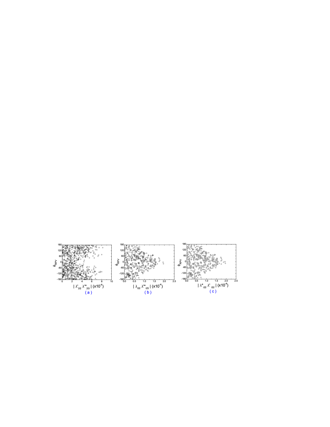
Figure 1: The allowed RPV parameter spaces with 500 GeV sfermions, and the RPV weak phase $(\phi_{RPV})$ is given in degree.

Table 1: Bounds for the relevant RPV coupling products by $B\to K^{(*)}\mu^{+}\mu^{-}$ and $B_{s}\to\mu^{+}\mu^{-}$ decays for 500 GeV sfermions, and previous bounds are listed for comparison.

Couplings	Bounds	Previous bounds [22]
$|\lambda^{\prime}_{2i2}\lambda^{\prime*}_{2i3}|$	$\leq 8.2\times 10^{-4}$	$\leq 11.5\times 10^{-4}$
$|\lambda_{i22}\lambda^{\prime*}_{i32}|$	$\leq 2.0\times 10^{-4}$	$\leq 4.5\times 10^{-4}$
$|\lambda^{*}_{i22}\lambda^{\prime}_{i23}|$	$\leq 2.0\times 10^{-4}$	$\leq 4.3\times 10^{-4}$

And the upper limits for the relevant RPV coupling products by $\mathcal{B}(B\to K^{(*)}\mu^{+}\mu^{-})$ and $\mathcal{B}(B_{s}\to\mu^{+}\mu^{-})$ are summarized in Table 1. For comparison, our previous bounds on these quadric coupling products are also listed. From Fig. 1 and Table 1, one can find that all three RPV coupling products are restricted, and the upper limits of $|\lambda_{i22}\lambda^{\prime*}_{i32}|$ and $|\lambda^{*}_{i22}\lambda^{\prime}_{i23}|$ are improved by about a factor of 2 by the new experimental data. Notice that we assume the masses of sfermions are 500 GeV. For other values of the sfermion masses, the bounds on the couplings in this paper can be easily obtained by scaling them by factor of $\tilde{f}^{2}\equiv(\frac{m_{\tilde{f}}}{500GeV})^{2}$.

Now we will analyze the constrained RPV effects on $\mathcal{B}(B_{s}\to\mu^{+}\mu^{-})$. The sensitivities of $\mathcal{B}(B_{s}\to\mu^{+}\mu^{-})$ to the constrained RPV couplings are shown in Fig. 2.

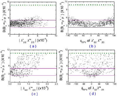
Figure 2: The constrained RPV coupling effects on $\mathcal{B}(B_{s}\to\mu^{+}\mu^{-})$. The olive (violet) horizontal dotted (solid) lines denote the limits of the 95% CL measurements (SM predictions).

The limits of the measurements at 95% CL and the SM predictions with $1\sigma$ theoretical uncertainties are also displayed in Fig. 2 for convenient comparison. Figs. 2 (a) and (b) show the constrained effects of the modulus and weak phase of t-channel squark exchange coupling $\lambda^{\prime}_{2i2}\lambda^{\prime*}_{2i3}$, respectively. As shown in Figs. 2 (a-b), with the contribution of $\lambda^{\prime}_{2i2}\lambda^{\prime*}_{2i3}$ included, $\mathcal{B}(B_{s}\to\mu^{+}\mu^{-})$ is lower than its experimental upper limit [5]. Besides the constraints from $\mathcal{B}(B_{s}\to K^{(*)}\mu^{+}\mu^{-})$, $\lambda^{\prime}_{2i2}\lambda^{\prime*}_{2i3}$ coupling is not further constrained by the new experimental upper limit from CMS and LHCb since its contribution to $\mathcal{B}(B_{s}\to\mu^{+}\mu^{-})$ is suppressed by $m^{2}_{\mu}/m^{2}_{B}$. Additionally, the allowed parameter space of $\lambda^{\prime}_{2i3}\lambda^{\prime*}_{2i2}$ would be excluded if the 68% CL experimental determination $\mathcal{B}(B_{s}\to\mu^{+}\mu^{-})=(1.8^{+1.1}_{-0.9})\times 10^{-8}$ [1] by the CDF Collaboration were taken as a constraint. Two s-channel sneutrino exchange contributions to $\mathcal{B}(B_{s}\to\mu^{+}\mu^{-})$ are very similar to each other. We would take the $\lambda_{i22}\lambda^{\prime*}_{i23}$ contribution as an example, which is shown by Figs. 2 (c-d). We can see that $\mathcal{B}(B_{s}\to\mu^{+}\mu^{-})$ is sensitive to both the modulus and phase of $\lambda_{i22}\lambda^{\prime*}_{i23}$, and $\mathcal{B}(B_{s}\to\mu^{+}\mu^{-})$ not only could be increased but also could be decreased by the presence of $\lambda_{i22}\lambda^{\prime*}_{i23}$ coupling. Generally, the $\lambda_{i22}\lambda^{\prime*}_{i23}$ coupling could alter $\mathcal{B}(B_{s}\to\mu^{+}\mu^{-})$ significantly since its contribution is not helicity suppressed by $m^{2}_{\mu}/m^{2}_{B}$. Thus, the constraint on $\lambda_{i22}\lambda^{\prime*}_{i23}$ is due to the bound of $\mathcal{B}(B_{s}\to\mu^{+}\mu^{-})$ [5].

Then we turn to analyzing the constrained RPV effects in $B\to K^{(*)}\mu^{+}\mu^{-}$ decays. Using the new constrained parameter spaces shown in Fig. 1, we will give the RPV effects on the dimuon invariant mass spectra and the forward-backward asymmetries of $B\to K^{(*)}\mu^{+}\mu^{-}$ decays.

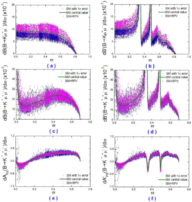
Figure 3: The effects of RPV coupling $\lambda^{\prime}_{2i2}\lambda^{\prime*}_{2i3}$ due to the squark exchange in $B\to K^{(*)}\mu^{+}\mu^{-}$ decays. The $\varpi$ denotes $\hat{s}$, magenta “$\times$” denotes the SM prediction within $1\sigma$ error ranges of the input parameters, olive solid line denotes the central value of the SM prediction, and blue “$\mid$” denotes the SUSY prediction. The same goes for Figs. 4, 5, 8, and 9.

Figure 4: $\mathcal{A}_{FB}(B\to K^{*}\mu^{+}\mu^{-})$ including RPV coupling $\lambda^{\prime}_{2i2}\lambda^{\prime*}_{2i3}$ versus the 95% CL data: CDF (blue dotted line), Belle (purple solid line), and LHCb (red dashed line).

In Fig. 3, we present correlations between the dimuon invariant mass spectra as well as the dimuon forward-backward asymmetries and the parameter spaces of $\lambda^{\prime}_{2i3}\lambda^{\prime*}_{2i2}$ by the two-dimensional scatter plots. The dimuon invariant mass distribution and the dimuon forward-backward asymmetry are given with vector meson dominance contribution excluded in terms of $d\mathcal{B}/d\hat{s}$ and $d\mathcal{A}_{FB}/d\hat{s}$, and included in $d\mathcal{B}^{\prime}/d\hat{s}$ and $d\mathcal{A}^{\prime}_{FB}/d\hat{s}$, respectively. In Fig. 3, the magenta “$\times$” denotes the SM prediction within $1\sigma$ error ranges of the input parameters, olive solid line denotes the central value of the SM prediction, and blue “$\mid$” denotes the RPV supersymmetry (SUSY) prediction including $\lambda^{\prime}_{2i2}\lambda^{\prime*}_{2i3}$ coupling within $1\sigma$ error ranges of the input parameters. The theoretical uncertainties of the SM predictions of $d\mathcal{B}(B\to K^{(*)}\mu^{+}\mu^{-})/d\hat{s}$ are quite large; nevertheless the theoretical uncertainties are canceled a lot in $d\mathcal{A}_{FB}(B\to K^{*}\mu^{+}\mu^{-})/d\hat{s}$.

The RPV effects on $d\mathcal{A}^{\prime}_{FB}(B\to K^{*}\mu^{+}\mu^{-})/d\hat{s}$ are shown in Fig. 3 (f). This observable has been measured as a function of the dimuon invariant mass square $q^{2}$ by BABAR [8], Belle [9], CDF [10], and LHCb [11], and the current situation is specially exemplified in Fig. 4. As shown in Fig. 4, the fitted $d\mathcal{A}^{\prime}_{FB}(B\to K^{*}\mu^{+}\mu^{-})/d\hat{s}$ from Belle is generally higher than the SM expectation in whole $q^{2}$ bins, and the CDF fitted result is consistent with the SM prediction in some $q^{2}$ bins and it is higher than the SM prediction in some other $q^{2}$ bins; nevertheless the LHCb fitted result, which is the most precise to data, is in good agreement with the SM prediction. Especially, in the region of $0\leq\hat{s}\leq 0.072$ (i.e., $0$ GeV${}^{2}\leq q^{2}\leq 2$ GeV²), the Belle measurement favors a positive value which is not confirmed by CDF and LHCb, whereas the sign of the SM prediction for $d\mathcal{A}^{\prime}_{FB}(B\to K^{*}\mu^{+}\mu^{-})/d\hat{s}$ is negative. One could find that the constrained RPV coupling $\lambda^{\prime}_{2i3}\lambda^{\prime*}_{2i2}$ still could accommodate $d\mathcal{A}_{FB}(B\to K^{*}\mu^{+}\mu^{-})/d\hat{s}$ from Belle, CDF, and LHCb at all $\hat{s}$ regions.

As for the s-channel sneutrino exchange couplings $\lambda_{i22}\lambda^{\prime*}_{i23}$ and $\lambda^{*}_{i22}\lambda^{\prime}_{i32}$, the constraints from $\mathcal{B}(B\to\mu^{+}\mu^{-})$ are rather restrictive.

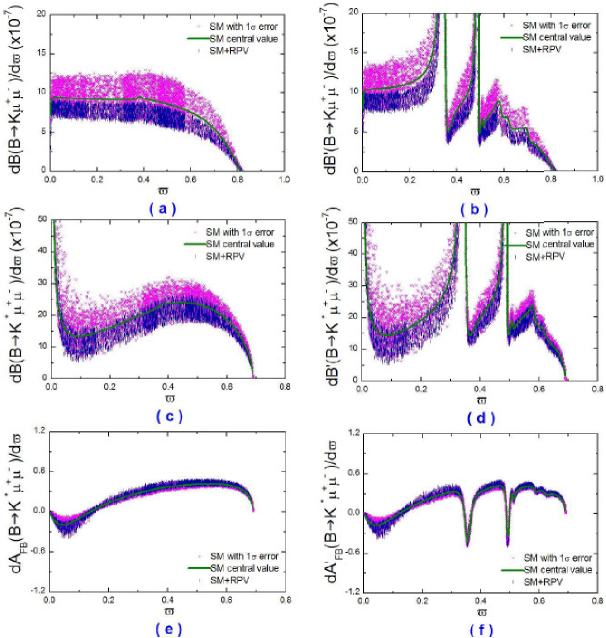
Figure 5: The effects of RPV coupling $\lambda_{i22}\lambda^{\prime*}_{i23}$ due to the sneutrino exchange in $B\to K^{(*)}\mu^{+}\mu^{-}$.

The $\lambda_{i22}\lambda^{\prime*}_{i23}$ coupling effects in $B\to K^{(*)}\mu^{+}\mu^{-}$ are displayed in Fig. 5; we see that $\lambda_{i22}\lambda^{\prime*}_{i23}$ coupling has negligible contribution to $d\mathcal{B}(B\to K^{(*)}\mu^{+}\mu^{-})/d\hat{s}$, and the differences between the SUSY prediction and the SM ones are due to the 95% CL experimental constraints. Nevertheless, constrained $\lambda_{i22}\lambda^{\prime*}_{i23}$ coupling has some effects on $d\mathcal{A}_{FB}(B\to K^{*}\mu^{+}\mu^{-})/d\hat{s}$. $\lambda^{*}_{i22}\lambda^{\prime}_{i32}$ coupling effects in $B\to K^{(*)}\mu^{+}\mu^{-}$ are similar to $\lambda_{i22}\lambda^{\prime*}_{i23}$ effects; thus we will not show them again.

3.2 RPC MI effects

Now we study RPC MI effects in $B_{s}\to\mu^{+}\mu^{-}$ and $B\to K^{(*)}\mu^{+}\mu^{-}$ decays in the MSSM with large tan$\beta$. The eight kinds of MIs $(\delta^{u,d}_{AB})_{23}$ with $(A,B)=(L,R)$ contribute to $B\to K^{(*)}\mu^{+}\mu^{-}$ decays, but only three kinds of MIs $(\delta^{u}_{LL})_{23}$, $(\delta^{d}_{LL})_{23}$, and $(\delta^{d}_{RR})_{23}$ contribute to $B_{s}\to\mu^{+}\mu^{-}$ decay. We will only consider the contributions of $(\delta^{u}_{LL})_{23}$, $(\delta^{d}_{LL})_{23}$, and $(\delta^{d}_{RR})_{23}$ MIs to $B_{s}\to\mu^{+}\mu^{-}$ and $B\to K^{(*)}\mu^{+}\mu^{-}$ decays in this work. We take the best-fit values of the constrained MSSM parameters from the LHC SUSY search results [31]: $m_{0}=450~{}GeV,m_{1/2}=780~{}GeV,A_{0}=-1110,$ $\mbox{sign}(\mu)>0$, and $\mbox{tan}\beta=41$. The experimental data shown in Eq. (17) will be used to constrain the three kinds of MI parameters.

MI coupling $(\delta^{u}_{LL})_{23}$ has some effects on $\mathcal{B}(B_{s}\to\mu^{+}\mu^{-})$ and $\mathcal{B}(B\to K^{(*)}\mu^{+}\mu^{-})$, and the bound of $(\delta^{u}_{LL})_{23}$ is obtained from both $\mathcal{B}(B_{s}\to\mu^{+}\mu^{-})$ and $\mathcal{B}(B\to K^{*}\mu^{+}\mu^{-})$. However, for $(\delta^{d}_{LL})_{23}$ and $(\delta^{d}_{RR})_{23}$ MI parameters, the constraints by $\mathcal{B}(B\to K^{(*)}\mu^{+}\mu^{-})$ are rather weak, which are mainly derived from $\mathcal{B}(B_{s}\to\mu^{+}\mu^{-})$.

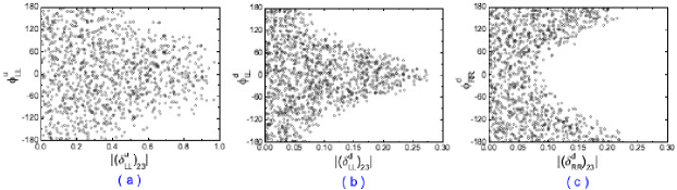
Figure 6: The allowed parameter spaces of $(\delta^{u}_{LL})_{23}$, $(\delta^{d}_{LL})_{23}$, and $(\delta^{d}_{RR})_{23}$ MI parameters constrained by $\mathcal{B}(B_{s}\to\mu^{+}\mu^{-})$ and $\mathcal{B}(B\to K^{(*)}\mu^{+}\mu^{-})$ at 95% CL, and the RPC phases are given in degree.

The constrained spaces of $(\delta^{u}_{LL})_{23}$, $(\delta^{d}_{LL})_{23}$, and $(\delta^{d}_{RR})_{23}$ are displayed in Fig. 6. As shown in Fig. 6, both phases and moduli of three MIs are obviously constrained by the branching ratios given in Eq. (17), and the bounds on the three moduli are $|(\delta^{u}_{LL})_{23}|\leq 1.0$, $|(\delta^{d}_{LL})_{23}|\leq 0.28$, and $|(\delta^{d}_{RR})_{23}|\leq 0.22$. Note that the very strong constraints on the phases of $(\delta^{d}_{LL,RR})_{23}$ MIs arise from $\Delta M_{s}$, $\Delta\Gamma_{s}$, and $\phi_{s}^{J/\psi\phi}$ [32], which are about $\phi^{d}_{LL,RR}\in[20^{\circ},80^{\circ}]\cup[-160^{\circ},-100^{\circ}]$ with $m^{2}_{\tilde{g}}/m^{2}_{\tilde{q}}=1$. If considering the strong constrained phases from $\Delta M_{s}$, $\Delta\Gamma_{s}$, and $\phi_{s}^{J/\psi\phi}$, we have $|(\delta^{d}_{LL})_{23}|\leq 0.24$ and $|(\delta^{d}_{RR})_{23}|\leq 0.22$.

Now we analyze the $(\delta^{u}_{LL})_{23}$, $(\delta^{d}_{LL})_{23}$, and $(\delta^{d}_{RR})_{23}$ MI effects on $\mathcal{B}(B_{s}\to\mu^{+}\mu^{-})$. The sensitivities of $\mathcal{B}(B_{s}\to\mu^{+}\mu^{-})$ to both moduli and phases of three MIs are displayed in Fig. 7.

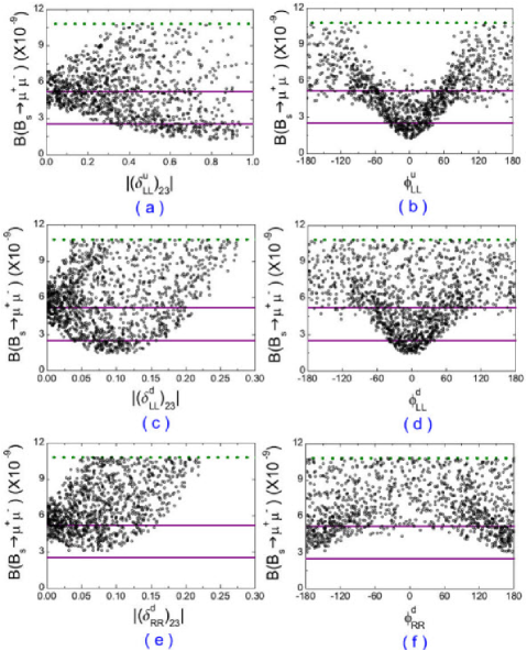
Figure 7: The constrained MI effects on $\mathcal{B}(B_{s}\to\mu^{+}\mu^{-})$. The olive (violet) horizontal dotted (solid) lines denote the limits of the 95% CL measurements (SM predictions with $1\sigma$ error bar).

As shown in Fig. 7, all three couplings are constrained by the upper limit of $\mathcal{B}(B_{s}\to\mu^{+}\mu^{-})$, and $\mathcal{B}(B_{s}\to\mu^{+}\mu^{-})$ has moderate sensitivities to both the moduli and phases. The minimum value of $\mathcal{B}(B_{s}\to\mu^{+}\mu^{-})$ may present when $|(\delta^{u}_{LL})_{23}|\geq 0.4$ and $|\phi^{d}_{LL}|\leq 45^{\circ}$, $|(\delta^{d}_{LL})_{23}|\in[0.05,0.15]$ and $|\phi^{d}_{LL}|\leq 45^{\circ}$ or $|(\delta^{d}_{RR})_{23}|\in[0.02,0.10]$ and $|\phi^{d}_{RR}|\geq 120^{\circ}$. The differences between the SUSY predictions at $|(\delta^{u,d}_{AB})_{23}|=0$ and the SM predictions come from contributions in the MSSM with the CKM matrix as the only source of flavor violation.

Then we analyze the constrained $(\delta^{u}_{LL})_{23}$, $(\delta^{d}_{LL})_{23}$, and $(\delta^{d}_{RR})_{23}$ MI effects in $B\to K^{(*)}\mu^{+}\mu^{-}$ decays. Using the constrained parameter spaces shown in Fig. 6, we will give the MSSM predictions to the dimuon invariant mass spectra of the decay width and the dimuon forward-backward asymmetries of $B\to K^{(*)}\mu^{+}\mu^{-}$ decays in the MI approximation. Besides the MI contributions, the SUSY predictions also include the contributions that come from graphs including SUSY Higgs bosons and sparticles in the limit in which we neglect all the MI contributions, which are called non-MI contributions, and the non-MI SUSY effects are shown in Fig. 8.

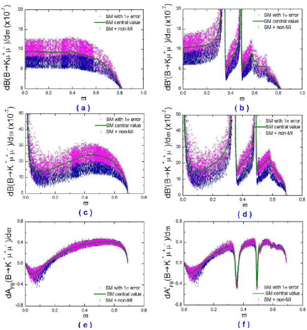
Figure 8: The constrained non-MI effects in $B\to K^{(*)}\mu^{+}\mu^{-}$ decays.

From Figs. 8 (a-b), we can see that $d\mathcal{B}(B\to K\mu^{+}\mu^{-})/d\hat{s}$ could be slightly suppressed at all $\hat{s}$ regions by the non-MI SUSY couplings. As shown in Figs. 8 (c-d), $d\mathcal{B}(B\to K^{*}\mu^{+}\mu^{-})/d\hat{s}$ could be decreased a lot at the middle $\hat{s}$ region by these couplings. Figs. 8 (e-f) show us that the non-MI SUSY couplings could slightly suppress $d\mathcal{A}_{FB}(B\to K^{*}\mu^{+}\mu^{-})/d\hat{s}$ at the middle $\hat{s}$ region.

The constrained $(\delta^{d}_{LL})_{23}$ and $(\delta^{d}_{RR})_{23}$ MIs have no obvious effects in $B\to K{(*)}\mu^{+}\mu^{-}$ decays. $(\delta^{u}_{LL})_{23}$ MI contributions to $B\to K^{(*)}\mu^{+}\mu^{-}$ are presented in Fig. 9. Note that the SUSY predictions in Fig. 8 also include the non-MI contributions shown in Fig. 8.

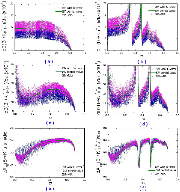
Figure 9: The constrained $(\delta^{u}_{LL})_{23}$ MI effects in $B\to K^{(*)}\mu^{+}\mu^{-}$ decays.

As shown in Figs. 9 (a-b), the constrained $(\delta^{u}_{LL})_{23}$ MI has no obvious effects on $d\mathcal{B}(B\to K\mu^{+}\mu^{-})/d\hat{s}$, which could be slightly suppressed at all $\hat{s}$ regions by only non-MI effects. On the other hand, its contribution to $B\to K^{*}\mu^{+}\mu^{-}$ could be significant, as shown in Figs. 9 (c-f), when theoretical uncertainties are considered. It is of interest to note that the contribution to $d\mathcal{A}_{FB}(B\to K^{*}\mu^{+}\mu^{-})/d\hat{s}$ is favored by the current experimental measurements from Belle, CDF, and LHCb [10, 9, 11].

4 Conclusions

Motivated by the recent searches of $\mathcal{B}(B_{s}\to\mu^{+}\mu^{-})$ by the CDF, LHCb, and CMS Collaborations, we have studied $B_{s}\to\mu^{+}\mu^{-}$ and $B\to K^{(*)}\mu^{+}\mu^{-}$ decays in the MSSM with and without R-parity. In the MSSM without R-parity, we have found that the bounds of sneutrino exchange RPV couplings are significantly improved by the present new measurements. The further constrained RPV coupling due to t-channel squark exchange still has significant effects in $B\to K^{(*)}\mu^{+}\mu^{-}$ decays, and the current measurements of $d\mathcal{A}_{FB}(B\to K^{*}\mu^{+}\mu^{-})/d\hat{s}$ could be accommodated by the squark exchange coupling. The further constrained couplings due to s-channel sneutrino exchange could have large effects in $B_{s}\to\mu^{+}\mu^{-}$, but have negligible effects in $B\to K^{(*)}\mu^{+}\mu^{-}$ decays.

In the MSSM with R-parity, three MI parameters $(\delta^{u}_{LL})_{23}$, $(\delta^{d}_{LL})_{23}$, and $(\delta^{d}_{RR})_{23}$ suffer the combined constraints from the present data of $\mathcal{B}(B_{s}\to\mu^{+}\mu^{-})$ and $\mathcal{B}(B\to K^{(*)}\mu^{+}\mu^{-})$. The constrained $(\delta^{u}_{LL})_{23}$ MI could give large contributions to $d\mathcal{A}_{FB}(B\to K^{*}\mu^{+}\mu^{-})/d\hat{s}$ at all $\hat{s}$ regions in favor of the current experimental measurements from Belle, CDF, and LHCb. The constrained $(\delta^{d}_{LL,RR})_{23}$ MIs have ignorable effects on the observables of $B\to K^{(*)}\mu^{+}\mu^{-}$decays. $d\mathcal{A}_{FB}(B\to K^{*}\mu^{+}\mu^{-})/d\hat{s}$ could be slightly decreased at the middle $\hat{s}$ region by the SUSY contributions which come from graphs including SUSY Higgs bosons and sparticles in the limit in which we neglect all the MI contributions.

In the immediate future, the LHC is expected to become sensitive to $\mathcal{B}(B_{s}\to\mu^{+}\mu^{-})$. Accurate measurements of the $B_{s}\to\mu^{+}\mu^{-}$ and $B\to K^{(*)}\mu^{+}\mu^{-}$ decays could further shrink or reveal the parameter spaces of MSSM with and without R-parity.

Appendix: Input parameters

The input parameters are summarized in Table 2. For the RPC MI effects, we take the five free parameters $m_{0}=450~{}GeV,m_{1/2}=780~{}GeV,A_{0}=-1110,$ $\mbox{sign}(\mu)>0$ and $\mbox{tan}\beta=41$ from Ref. [31]. All other MSSM parameters are then determined according to the constrained MSSM scenario as implemented in the program package SUSPECT [34]. For the form factors involving the $B\to K^{(*)}$ transitions, we will use the recent light-cone QCD sum rules results [35, 36], which are renewed with radiative corrections to the leading twist wave functions and SU(3) breaking effects. For the $q^{2}$ dependence of the form factors, they can be parameterized in terms of simple formulas with two or three parameters. The expression can be found in Refs. [35, 36]. In our numerical data analysis, the uncertainties induced by $F(0)$ are also considered.

Table 2: Default values of the input parameters.

$m_{B_{s}}=5.370~{}GeV,~{}~{}m_{B_{d}}=5.279~{}GeV,~{}~{}m_{B_{u}}=5.279~{}GeV,~{}~{}m_{W}=80.425~{}GeV,$
$m_{K^{\pm}}=0.494~{}GeV,~{}~{}m_{K^{0}}=0.498~{}GeV,~{}~{}m_{K^{*\pm}}=0.892~{}GeV,~{}~{}m_{K^{*0}}=0.896~{}GeV,$
$\overline{m}_{b}(\overline{m}_{b})=(4.19^{+0.18}_{-0.06})~{}GeV,~{}~{}\overline{m}_{s}(2GeV)=(0.100^{+0.030}_{-0.020})~{}GeV,$
$\overline{m}_{u}(2GeV)=0.0017\sim 0.0031~{}GeV,~{}\overline{m}_{d}(2GeV)=0.0041\sim 0.0057~{}GeV,$
$m_{e}=0.511\times 10^{-3}~{}GeV,~{}~{}m_{\mu}=0.106~{}GeV,$   $m_{t,pole}=172.9\pm 1.1~{}GeV.$	[25]
$\tau_{B_{s}}=(1.466\pm 0.059)~{}ps,~{}~{}\tau_{B_{d}}=(1.530\pm 0.009)~{}ps,~{}~{}\tau_{B_{u}}=(1.638\pm 0.011)~{}ps.$	[25]
$|V_{tb}|\approx 0.99910,~{}~{}|V_{ts}|=0.04161^{+0.00012}_{-0.00078}.$	[25]
$\mbox{sin}^{2}\theta_{W}=0.22306,~{}~{}\alpha_{e}=1/137.$	[25]
$f_{B_{s}}=0.230\pm 0.030~{}GeV.$	[33]

References

- [1] T. Aaltonen et al. (CDF Collaboration), Phys. Rev. Lett. 107, 191801 (2011).
- [2] S. Chatrchyan et al. (CMS Collaboration), Phys. Rev. Lett. 107, 191802 (2011).
- [3] R. Aaij et al. (LHCb Collaboration), Phys. Lett. B 708, 55 (2012).
- [4] R. Aaij et al. (LHCb Collaboration), Phy. Lett. B699 330 (2011).
- [5] CMS and LHCb Collaborations, CMS-PAS-BPH-11-019, LHCb-CONF-2011-047, CERN-LHCb-CONF-2011-047.
- [6] V. Abazov et al. (DØ Collaboration), Phys. Lett. B693, 539 (2010); T. Aalonen et al. (CDF Collaboration), Phys. Rev. Lett. 100, 101802 (2008).
- [7] A. J. Buras, M. V. Carlucci, S. Gori and G. Isidori, JHEP 1010, 009 (2010).
- [8] B. Aubert et al. (BABAR Collaboration), Phys. Rev. D79, 031102 (2009).
- [9] J. T. Wei et al. (Belle Collaboration), Phys. Rev. Lett. 103, 171801 (2009).
- [10] T. Aaltonen et al. (CDF Collaboration), Phys. Rev. Lett. 108, 081807 (2012).
- [11] R. Aaij et al. (LHCb Collaboration), arXiv:1112.3515.
- [12] D. Palle, arXiv:1111.1639.
- [13] C. Beskidt et al., Phys. Lett. B705, 493 (2011).
- [14] A. G. Akeroyd, F. Mahmoudi and D. M. Santos, JHEP 1112, 088 (2011).
- [15] W. Altmannshofer, M. Carena, S. Gori and A. de la Puente, arXiv:1107.3814.
- [16] A. K. Alok et al., JHEP 1111, 121 (2011).
- [17] E. Lunghi and A. Soni, JHEP 1011, 121 (2010).
- [18] Q. Chang, X. Q. Li and Y. D. Yang, JHEP 1004, 052 (2010).
- [19] W. Altmannshofer et al., Nucl. Phys. B830, 17-94 (2010).
- [20] W. Altmannshofer et al., JHEP 0901, 019 (2009).
- [21] A. K. Alok and S. K. Gupta, Eur. Phys. J. C65, 491 (2010).
- [22] Y. G. Xu, R. M. Wang and Y. D. Yang, Phys. Rev. D74, 114019 (2006).
- [23] F. Gabbiani, E. Gabrielli, A. Masiero and L. Silvestrini, Nucl. Phys. B477, 321 (1996).
- [24] F. Gabbiani and A. Masiero, Nucl. Phys. B322, 235 (1989).
- [25] K. Nakamura et al. (Particle Data Group), J. Phys. G37, 075021 (2010) and 2011 partial update for the 2012 edition.
- [26] C. Bobeth, T. Ewerth, F. Kruger and J. Urban, Phys. Rev. D64, 074014 (2001).
- [27] A. Ali, P. Ball, L. T. Handoko and G. Hiller, Phys. Rev. D61, 074024 (2000).
- [28] E. Lunghi, A. Masiero, I. Scimemi and L. Silvestrini, Nucl. Phys. B568, 120-144 (2000).
- [29] P. Cho, M. Misiak and D. Wyler, Phys. Rev. D54, 3329-3344 (1996).
- [30] J. L. Hewett and J. D. Wells, Phys. Rev. D 55, 5549 (1997).
- [31] S. Heinemeyer, arXiv:1202.1991 [hep-ph].
- [32] R. M. Wang, Y. G. Xu, Q. Chang and Y. D. Yang, Phys. Rev. D83, 095010 (2011).
- [33] S. Hashimoto, Int. J. Mod. Phys. A20, 5133-5144 (2005).
- [34] A. Djouadi, J. L. Kneur and G. Moultaka, Comput. Phys. Commun. 176, 426 (2007).
- [35] P. Ball and R. Zwicky, Phys. Rev. D71, 014015 (2005).
- [36] P. Ball and R. Zwicky, Phys. Rev. D71, 014029 (2005).