Abundances in HD 27411 and the helium problem in Am stars

Abstract

We analyze a high-resolution spectrum of the A3m star HD 27411. We compare abundances derived from ATLAS9 model atmospheres with those using the more computationally-intensive ATLAS12 code. We found very little differences in the abundances, suggesting that ATLAS9 can be used for moderate chemical peculiarity. Our abundances agree well with the predictions of diffusion theory, though for some elements it was necessary to calculate line profiles in non-thermodynamic equilibrium to obtain agreement. We investigate the effective temperatures and luminosities of Am/Fm stars using synthetic Strömgren indices derived from calculated spectra with the atmospheric abundances of HD 27411. We find that the effective temperatures of Am/Fm stars derived from Strömgren photometry are reliable, but the luminosities are probably too low. Caution is required when deriving the reddening of these stars owing to line blanketing effects. A comparison of the relative proportions of pulsating and non-pulsating Am stars with $\delta$ Scuti stars shows quite clearly that there is no significant decrease of helium in the driving zone, contrary to current models of diffusion.

1 Introduction

The “metallic-lined” or Am stars are A-type stars which have strong absorption lines of some metals such as Zn, Sr, Zr and Ba and weaker lines of other metals such as Ca and/or Sc relative to their spectral type as determined by the strength of the hydrogen lines (Preston, 1974). The strong metallic lines are more typical of an F star rather than an A star. The work of Michaud (1970) established radiative diffusion in a strong magnetic field as the likely cause of the chemical peculiarities in Ap stars. When the magnetic field is absent, diffusion leads to the Am/Fm stars (Watson, 1971). The presence of magnetic fields in Am stars has been investigated, but with negative results, (e.g. Fossati et al. (2007)). A peculiarity of Am stars is that their projected rotational velocities are generally much smaller than normal A stars and they are nearly always members of close binary systems. Rotational braking by tidal friction in a binary system is regarded as a possible explanation for the low rotational velocities in Am stars. Slow rotation further assists the segregation of elements by diffusion.

The abundance anomalies predicted by the diffusion hypothesis are usually much larger than observed. Richer, Michaud & Turcotte (2000) developed detailed models of the structure and evolution of Am/Fm stars using OPAL opacities, taking into account atomic diffusion and the effect of radiative acceleration. These models develop a convective zone due to ionization of iron-group elements at a temperature of approximately 200,000 K. In addition to this convective zone, these stars also have a thin superficial convective zone in which H and Hei are partially ionized. By assuming sufficient overshoot due to turbulence, these separate convective zones become one large convective zone. The resulting mixing dilutes the large abundance anomalies predicted by previous model, leading to abundances which closely resemble those observed in Am/Fm stars.

A detailed abundance analysis of eight Am stars belonging to the Praesepe cluster (Fossati et al., 2007) show good agreement with the predictions of Richer, Michaud & Turcotte (2000) for almost all the common elements except for Na and possibly S. The models of Richer, Michaud & Turcotte (2000) assume a certain ad-hoc parametrization of turbulent transport coefficients which are adjusted to reproduce observations. Other parameterizations of turbulence have been proposed for other types of stars. Talon et al. (2006) have investigated to what extent these are consistent with the anomalies observed on Am/Fm stars. They find that the precision of current abundances is insufficient to distinguish between models. More recently, Michaud et al. (2011) have studied the abundance anomalies of the mild Am star Sirius A. They find that except for B, N and Na, there is good agreement with the predicted anomalies but turbulent mixing or mass loss is required. It is not clear whether it is turbulence or mass loss which competes with diffusion to lower the abundance anomalies. For example, Vick et al. (2011) find that diffusion in the presence of weak mass loss can explain the observed abundance anomalies of pre-main-sequence stars. This is in contrast to turbulence models which do not allow for abundance anomalies to develop on the pre-main-sequence.

Most of the pulsational driving in $\delta$ Scuti stars is caused by the $\kappa$ mechanism operating in the Heii ionization zone. Diffusion tends to drain He from this zone and therefore pulsational driving may be expected to be weaker or absent in Am/Fm stars (Baglin, 1972). In fact, for many years it was thought that classical Am/Fm stars did not pulsate, though claims were made for some stars (Kurtz, 1989). Recently, intensive ground-based observations by SUPER-WASP (Smalley et al., 2011), and also from the Kepler mission (Balona et al., 2011) have shown that many Am/Fm stars do pulsate. Smalley et al. (2011), for example, found that about 200 Am/Fm stars out of a total of 1600 (12.5 percent) show $\delta$ Sct pulsations, but with generally lower amplitudes. They found that the pulsating Am/Fm stars are confined between the red and blue radial fundamental edges, in agreement with Balona et al. (2011). While there are many $\delta$ Sct stars hotter than the fundamental blue edge, this does not seem to be the case for pulsating Am/Fm stars. The significance of this result remains to be evaluated.

The effect of draining of He from the Heii ionization zone is to reduce the width of the instability strip, the blue edge moving towards the red edge, eventually leading to the disappearance of the instability strip when He is sufficiently depleted (Cox et al., 1979). Turcotte et al. (2000) has discussed the effect of diffusion on pulsations in Am/Fm stars using the models by Richer, Michaud & Turcotte (2000). One significant difference with earlier models is that a substantial amount of He remains in the Heii ionization zone. The blue edge of the instability strip for Am/Fm stars is sensitive to the magnitude of the abundance variations and is thus indicative of the depth of mixing by turbulence. Turcotte et al. (2000) predict that pulsating Am/Fm stars should lie in a confined region of the HR diagram close to the red edge of the $\delta$ Sct instability strip. However, Balona et al. (2011) show that there is no relationship between the predicted Am/Fm instability strip and the actual location of these stars in the HR diagram.

A particularly interesting result of the pulsation analysis of Turcotte et al. (2000) is the prediction of long-period g modes in A-type stars. As the star evolves, the driving regions shift deeper into the star and the g modes become gradually more and more excited. Whereas p modes are stabilized through diffusion, g modes tend to be excited as a result of that process. It appears that diffusion may act to enhance driving of long-period g modes due to a significant increase in opacity due to iron-group elements. This may have a bearing on the fact that nearly all A-type stars observed by Kepler have unexplained low-frequencies (Balona, 2011).

When dealing with objects with non-standard chemical composition, such as Am stars, it is crucial that the opacities are correctly calculated. This question has been investigated by several authors in recent years. These studies show that a non-standard chemical composition of the stellar atmosphere alters the flux distribution of the star or modifies the profiles of the Balmer lines (Leone & Manfré (1997), Catanzaro, Leone & Dall (2004)). Therefore a determination of T_eff and $\log g$ based on a comparison between observed and computed Balmer-line profiles will not be correct unless one takes into account the metallicity of the star. Thus, even estimates based on standard analysis of the spectra may be in error when applied to Am/Fm stars.

In this paper, we investigate the determination of effective temperature and surface gravity of the Am star HD 27411 (HR 1353, A3m) using spectra in the ESO archives. The purpose is to determine whether the stellar parameters of this star agree with those obtained from Strömgren photometry and hence to test the reliability of the effective temperature calibration applied to Am/Fm stars. The star was used by Ryabchikova, Kochukhov & Bagnulo (2008) as a comparison in their study on the calcium stratification in Ap stars. HD 27411 is not known to pulsate. However, as we know from Kepler observations, pulsations in A and F stars with amplitudes too low to be detected from the ground are common.

Atmospheric models obtained with ATLAS9 (Kurucz, 1993) use precomputed line opacities in the form of opacity distribution functions (ODFs). These are tabulated for multiples of the solar metallicity and for various microturbulent velocities. This approach allows very fast computation of model atmospheres, but with very little flexibility in choice of chemical profile and microturbulent velocity. While this is satisfactory for most applications, it fails for chemically peculiar stars where a non-standard chemical composition profile is required. This can be done with ATLAS12 (Kurucz, 1997), which is essentially identical to ATLAS9, but uses the opacity sampling (OS) method to evaluate line opacities. In this study we compare the abundances of HD 27411 obtained with both codes to determine if the use of ATLAS12 is essential.

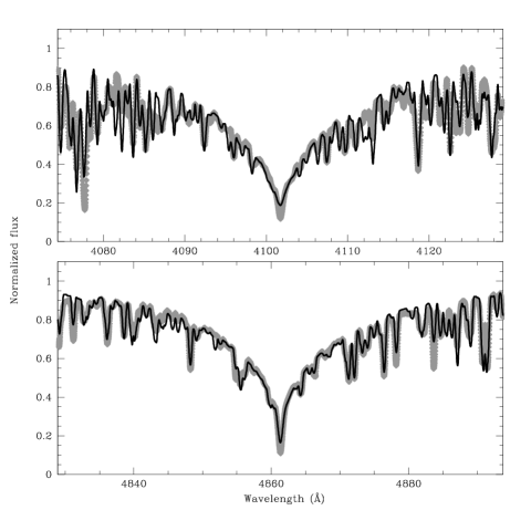
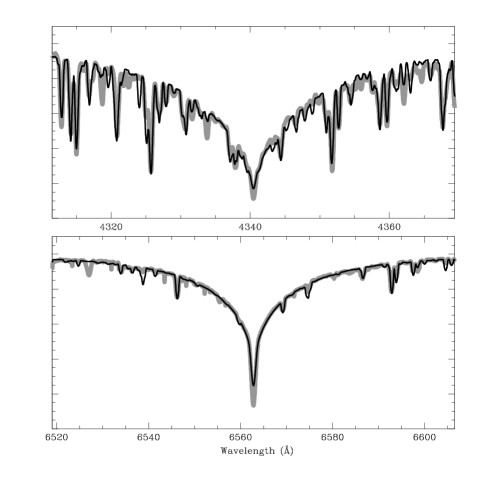
Figure 1: Comparison between the observed (crosses) and computed (solid red line) hydrogen line profiles. From top to bottom: the Balmer line profiles from H_δ to H_α. The synthetic profiles were computed with SYNTHE using an ATLAS12 model atmosphere with T_eff = 7400 $\pm$ 150 K, $\log g$ = 4.0 $\pm$ 0.1, $\xi$ = 4.2 $\pm$ 0.3 km s^-1, $v_{e}\sin i$ = 20.5 $\pm$ 0.5 km s^-1 and individual abundances shown in Table 2.

The result that Am stars are not confined to particular region of the $\delta$ Sct instability strip depends, to a large extent, on effective temperatures and luminosities estimated from Strömgren photometry (Smalley et al., 2011). It is not clear whether the calibration, derived from normal AF stars, can be applied to Am/Fm stars. In this paper we use synthetic Strömgren photometry applied to models of Am/Fm stars to investigate the reliability of fundamental parameters estimated from the photometry. Finally, we discuss the relative numbers of pulsating and non-pulsating Am stars and compare these to the relative numbers of $\delta$ Scuti and constant stars in the instability strip. From this comparison, one can deduce the effectiveness of pulsational driving in the Heii ionization zone and compare the He abundance to that expected from diffusion calculations.

Table 1: Ions used to determine the microturbulent velocity in HD 27411. The number of spectral lines used, the microturbulent velocity, $\xi$, the derived abundance and the radial velocity, RV, are listed.

Elem	N	$\xi$	Abundance	RV
		km s-1	$\log N_{\rm el}/N_{\rm Tot}$	km s-1
Fei	71	3.9 $\pm$ 0.3	$-$3.80 $\pm$ 0.03	40.4 $\pm$ 0.6
Feii	15	4.4 $\pm$ 0.2	$-$3.84 $\pm$ 0.04	40.9 $\pm$ 0.6
Nii	24	4.4 $\pm$ 0.6	$-$4.63 $\pm$ 0.03	40.5 $\pm$ 1.3
Adopted	–	4.2 $\pm$ 0.3	–	40.6 $\pm$ 0.3

2 Observation and data analysis

The spectrum of HD 27411 is available in the ESO archive as a part of the UVES Paranal Observatory Project (UVES POP), which aims to create a library of high-resolution spectra across the HR diagram (Bagnulo et al., 2003). The spectrum was obtained in 2002, September 18 with a resolving power of R = 80 000.

In order to determine the optimal parameters, we minimize the difference between the observed and synthetic spectrum. Thus we minimize

$$\chi^{2}=\frac{1}{N}\sum\left(\frac{I_{\rm obs}-I_{\rm th}}{\delta I_{\rm obs}}\right)^{2}$$

where $N$ is the total number of points, $I_{\rm obs}$ and $I_{\rm th}$ are the intensities of the observed and computed profiles, respectively, and $\delta I_{\rm obs}$ is the photon noise. Synthetic spectra were generated in three steps. Firstly, we computed a model atmosphere using the ATLAS9 code. The stellar spectrum was then synthesized using SYNTHE (Kurucz & Avrett, 1981). Finally, the spectrum was convolved with the instrumental and rotational profiles.

As starting values of T_eff and $\log g$, we used the values derived from Strömgren photometry: $V=6.075\pm 0.007$, $b-y=0.164\pm 0.004$, $m_{1}=0.249\pm 0.015$, $c_{1}=0.847\pm 0.007$, $\beta=2.813\pm 0.005$ (Hauck & Mermilliod, 1998). Using the algorithm in Moon (1985) to obtain the reddening, we obtain $V_{0}=5.972$, $(b-y)_{0}=0.140$, $m_{0}=0.256$, $c_{0}=0.842$. Note, however, that because of increased line blanketing in HD 27411 relative to normal stars, it is not clear if the de-reddening procedure can be applied (see below). Using these values, the calibration of Moon & Dworetsky (1985) leads to T_eff = 7820 K and $\log g$ = 4.12, while the calibration of Balona (1994) gives T_eff = 7760 K, $\log g$ = 4.11. Again, because of increased line blanketing, these must be taken merely as provisional values. We adopt T_eff = 7800 K, $\log g$ = 4.12.

To decrease the number of parameters, we computed the $v_{e}\sin i$ of HD 27411 by matching synthetic line profiles from SYNTHE to a number of metallic lines. The Mgi triplet at $\lambda\lambda$5167-5183 Å is particularly useful for this purpose. The best fit was obtained with $v_{e}\sin i$ = 20.5 $\pm$ 0.5 km s^-1. This value is in good agreement with $v_{e}\sin i$ = 20.4 $\pm$ 0.4 km s^-1 by Diaz et al. (2011).

To determine stellar parameters as consistently as possible with the actual structure of the atmosphere, we performed the abundance analysis by the following iterative procedure:

(i) $T_{\rm eff}$ is estimated by computing the ATLAS9 model atmosphere which gives the best match between the observed H_δ, H_γ, H_β, and H_α line profiles and those computed with SYNTHE. $\log g$ is estimated by matching the observed and calculated profiles of the Mgi triplet at $\lambda\lambda$ 5167–5183 Å which is extremely sensitive to gravity. This leads to T_eff = 7600 $\pm$ 150 K, $\log g$ = 4.0 $\pm$ 0.1, and ODF = [+0.5].

(ii) The microturbulent velocity, $\xi$, is determined independently from three sets of spectral lines: 71 lines from Fei, 15 lines from Feii, and 24 lines from Nii. For this purpose we used all lines with equivalent width (EW) $>$ 10 mÅ. In particular, $\xi$ is computed by requiring that the derived abundances do not depend on the measured equivalent widths. To convert equivalent widths to abundances we used the WIDTH9 code (Kurucz & Avrett, 1981). Values of $\xi$, the abundance and the radial velocity obtained for each ion are listed in Table 1. The adopted microturbulence is in agreement with Landstreet et al. (2009) (see Fig. 2 of their paper). The effective temperature is in agreement with the equilibrium condition between Fei and Feii, since the iron abundances derived separately from these two different ionization stages are in good agreement.

(iii) The projected rotational velocity is relatively high. To overcome line blending problems, we divided the spectrum into a number of sub-intervals $\approx$25 Å wide. For each interval we performed a separate synthesis analysis. We used the abundances of Fe and Ni given in Table 1 as starting values in this procedure. The atomic parameters adopted in this analysis are from Kurucz & Bell (1995) with line lists subsequently updated by Castelli & Hubrig (2004). The adopted abundances, shown in the second column of Table 2, are weighted averages expressed in the usual form $\log N_{\rm el}/N_{\rm Tot}$.

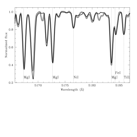
Figure 2: Comparison between observed (crosses) and computed (solid red line) spectra in the region of the Mgib triplet, $\lambda\lambda$5167.321, 5172.684, and 5183.604. The stellar parameters are T_eff = 7400 K, $\log g$ = 4.0, and $\log Mg/N_{\rm tot}$ = $-$4.58 $\pm$ 0.18.

Values of T_eff, $\log g$, $\xi$ and individual abundances estimated in this way were then used as initial guesses for starting another iterative procedure based on the ATLAS12 code. The best fit was obtained after three iterations and led to the following parameters: T_eff = 7400 $\pm$ 150 K, $\log g$ = 4.0 $\pm$ 0.1, $\xi$ = 4.2 $\pm$ 0.3 km s^-1 and $v_{e}\sin i$ = 20.5 $\pm$ 0.5 km s^-1. The corresponding abundances are shown in the second column of Table 2. Ryabchikova, Kochukhov & Bagnulo (2008) analyzed HD 27411 in a study of Ap stars and derived the following parameters: T_eff = 7650 K, $\log g$ = 4.0, $v_{e}\sin i$ = 18.5 km s^-1, and $\xi$ = 2.5 km s^-1. Considering the experimental errors, these values are in agreement with ours.

The fits between the observed and synthetic Balmer lines are shown in Fig. 1. The determination of surface gravity was constrained by using the Mgi triplet at $\lambda\lambda$ 5167–5183 Å, as shown in Fig. 2. Errors in T_eff and $\log g$ were estimated by the change in parameter values which leads to an increase of $\chi^{2}$ by unity (Lampton et al., 1976).

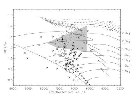
Figure 3: Location of HD 27411 in the HR diagram together with evolutionary tracks and isochrones for $\log t$ ranging from 8.87 to 8.95 (step 0.02 and $t$ in yrs). Asterisks are the pulsating AmFm stars taken from Smalley et al. (2011). The gray area is the approximate location of pulsating Am star models incorporating heavy-metal diffusion (Turcotte et al., 2000).

Table 2: Comparison among atmospheric parameters and abundances derived by ATLAS9 modeling and by ATLAS12 approach. The measurement without error is to be considered only as upper limit. In the last column we reported abundances derived with NLTE approach. All the abundances are expressed in the usual form $\log N_{\rm el}/N_{\rm Tot}$.

	A9	A12	A12+SYNSPEC
Teff	7600 $\pm$ 150	7400 $\pm$ 150	7400 $\pm$ 150
$\log g$	4.0 $\pm$ 0.1	4.0 $\pm$ 0.1	4.0 $\pm$ 0.1
Li	$-$8.35 $\pm$ 0.10	$-$8.42 $\pm$ 0.10
C	$-$3.97 $\pm$ 0.13	$-$3.90 $\pm$ 0.16
N	$-$4.60	$-$4.50
O	$-$3.55 $\pm$ 0.15	$-$3.70 $\pm$ 0.10
Na	$-$5.10 $\pm$ 0.19	$-$5.50 $\pm$ 0.19	$-$5.70 $\pm$ 0.10
Mg	$-$4.46 $\pm$ 0.13	$-$4.58 $\pm$ 0.18
Al	$-$5.11 $\pm$ 0.17	$-$5.05 $\pm$ 0.19	$-$5.44 $\pm$ 0.10
Si	$-$4.21 $\pm$ 0.16	$-$4.19 $\pm$ 0.10	$-$4.49 $\pm$ 0.12
S	$-$4.54 $\pm$ 0.14	$-$4.52 $\pm$ 0.18	$-$4.75 $\pm$ 0.10
K	$-$6.85 $\pm$ 0.10	$-$6.70 $\pm$ 0.10
Ca	$-$6.01 $\pm$ 0.18	$-$6.05 $\pm$ 0.14
Sc	$-$9.23 $\pm$ 0.10	$-$9.15 $\pm$ 0.17
Ti	$-$6.80 $\pm$ 0.15	$-$6.80 $\pm$ 0.17
V	$-$7.33 $\pm$ 0.17	$-$7.05 $\pm$ 0.18
Cr	$-$5.72 $\pm$ 0.13	$-$5.70 $\pm$ 0.15	$-$5.95 $\pm$ 0.10
Mn	$-$6.27 $\pm$ 0.10	$-$6.18 $\pm$ 0.17
Fe	$-$4.07 $\pm$ 0.12	$-$4.19 $\pm$ 0.13
Co	$-$6.07 $\pm$ 0.11	$-$6.19 $\pm$ 0.17
Ni	$-$5.00 $\pm$ 0.15	$-$5.03 $\pm$ 0.11
Cu	$-$6.93 $\pm$ 0.16	$-$6.94 $\pm$ 0.11
Zn	$-$6.67 $\pm$ 0.10	$-$6.70 $\pm$ 0.18
Y	$-$8.77 $\pm$ 0.10	$-$8.84 $\pm$ 0.18
Zr	$-$8.74 $\pm$ 0.10	$-$8.50 $\pm$ 0.15
Ba	$-$9.01 $\pm$ 0.18	$-$9.15 $\pm$ 0.15
La	$-$9.22 $\pm$ 0.11	$-$8.70 $\pm$ 0.15
Ce	$-$8.83 $\pm$ 0.15	$-$8.55 $\pm$ 0.15
Nd	$-$9.37 $\pm$ 0.06	$-$9.32 $\pm$ 0.10
Sm	$-$9.53 $\pm$ 0.06	$-$9.47 $\pm$ 0.09
Eu	$-$10.07 $\pm$ 0.05	$-$9.98 $\pm$ 0.14

3 Fundamental astrophysical quantities

If we adopt $T_{\rm eff}=7400\pm 150$ K and $\log g=4.00\pm 0.10$ from our spectroscopic analysis, we may use the relationships by Torres et al. (2010) to derive $\log L/L_{\odot}=0.99\pm 0.12$. These relate the mass and radius of a star to the effective temperature and gravity through empirical calibrations. The greatest source of uncertainty is the surface gravity determination.

The Hipparcos parallax for HD 27411, $\pi$ = 11.13 $\pm$ 0.38 (Van Leeuwen, 2007), is useful in refining the location of the star in the HR diagram. We show below that some caution is required in estimating reddening in Am/Fm stars and that HD 27411 is not significantly reddened. We therefore adopt $V_{0}=6.075$, which gives an absolute magnitude $M_{V}=1.31\pm 0.08$ where the error is derived from the error in the parallax. If we adopt the bolometric correction BC = 0.051 derived from Balona (1994), we have $M_{\rm bol}=1.36\pm 0.09$. Using M_bol,⊙ = 4.74 (Drilling & Landolt, 1999), we obtain $\log(L/L_{\odot})=1.35\pm 0.07$. From the luminosity and using $T_{\rm eff}$ = 7400 K, we obtain $R/R_{\odot}=2.88\pm 0.10$. The surface gravity obtained by using the parameters derived from the parallax and assuming a mass of about $2.17\pm 0.05~{}M_{\odot}$ is $\log g\approx 3.9\pm 0.1$. All the astrophysical quantities derived here are summarized in Table 3.

The location of the star in the HR diagram, together with some evolutionary tracks computed for non-solar metallicity Z = 0.03 (Girardi et al., 2000), is shown in Fig. 3. Also shown are isochrones computed by Marigo et al. (2008) for the same Z and for five ages, i.e. $\log t$ = 8.87, 8.89, 8.91, 8.93 and 8.95 ($t$ in years). The non-solar metallicity follows from our abundance analysis, and Z=0.03 is the nearest metallicity in the models computed by Girardi et al. (2000) and Marigo et al. (2008). The location of the star indicates a mass M $\approx$2 M_⊙ and an age of $t\approx$ 810 $\pm$ 40 Myrs.

In Table 3 we summarized all the astrophisical quantities for HD 27411.

It is well known that the vast majority of Am stars are binaries. There are few radial velocity measurements of HD 27411 in the literature. We could only find three measurements in Buscombe (1963): +17, +34 and $-$53 km s^-1. From our spectrum, we derived a radial velocity RV = +40.6 $\pm$ 0.3 km s^-1, which is a weighted average of the single velocities derived by converting the shift between observed and theoretical $\lambda_{c}$ from the species reported in Tablle 1. The scatter in these values does, indeed, suggest that HD 27411 is a binary. If so, then the companion is probably much fainter than the primary, otherwise one may expect to see some evidence in the spectrum.

Table 3: Astrophysical quantities for HD 27411. The second column are quantities derived from the parallax. The third column are quantities derived from Strömgren photometry and the last column from spectroscopy.

Paramerter	Parallax	Strömgren	Spectroscopy
$\pi$	$11.13\pm 0.38$
$V_{0}$	$6.075\pm 0.007$	$5.972\pm 0.005$
MV	$1.31\pm 0.08$
Mbol	$1.36\pm 0.09$
Teff		$7800\pm 200$	$7400\pm 150$
$\log(L/L_{\odot})$	$1.35\pm 0.07$	$0.96\pm 0.15$	$0.99\pm 0.12$
$\log g$	$3.9\pm 0.1$	$4.12\pm 0.10$	$4.00\pm 0.10$
R/R⊙	$2.88\pm 0.10$	$1.91\pm 0.27$	$1.90\pm 0.26$
$M/M_{\odot}$	$2.17\pm 0.05$	$1.77\pm 0.07$	$1.66\pm 0.07$

4 Abundances

In Fig. 4 we compare the LTE abundances derived from model atmospheres computed using ATLAS9 and ATLAS12. It is evident that there is good agreement in the abundances derived with the two different codes. There are some very small differences for Na, V, Zr and Nd, but these are only 0.1 dex or less. Thus we may use the faster ATLAS9 code with confidence. In Fig. 5 we show the abundances relative to solar standard abundances (Grevesse et al., 2010). The chemical pattern displayed here is typical of that observed in Am stars, i.e. an underabundance of C, N, O, Ca and Sc and a general increasing overabundance for heavy elements.

The atmospheric abundance of Li is interesting in the context of diffusion. Burkhart & Coupry (1991) and Burkhart et al. (2005) find that, in general, the Li abundance in Am stars is close to the cosmic value ($\log N_{\rm Li}/N_{\rm Tot}\approx-9.04$ dex), although some Am/Fm stars appear to have an underabundance of Li. Normal A-type stars in the range $7000<T_{\rm eff}<8500$ K appear to have a higher Li abundance, i.e. $\log N_{\rm Li}/N_{\rm Tot}\approx-8.64$ dex, (Burkhart & Coupry, 1995). To determine the Li abundance, we used the Lii $\lambda$6707 Å line, taking into account the hyperfine structure (Andersen, Gustafson & Lambert, 1984). The abundance that gives the best fit is $\log N_{\rm Li}/N_{\rm Tot}$ = $-$8.42$\pm$0.10, which is closer to the abundance in normal A stars and agrees with the average Li abundance of three cluster Am/Fm stars observed by Fossati et al. (2007).

Richer, Michaud & Turcotte (2000) predict abundances as a function of stellar age and effective temperature using their models of diffusion. Fig. 14 of their paper allows us to estimate the predicted abundances for a star with a given T_eff up to a maximum age of $\approx$ 670 Myrs. We find that age of HD 27411 to be about $810\pm 40$ Myr, which is considerably older than the maximum age of models in Richer, Michaud & Turcotte (2000), but we will assume that models of 670 Myr still give a fair approximation of the abundances. For T_eff = 7400 K, which is our best estimate for HD 27411, the models by Richer, Michaud & Turcotte (2000) predicts underabundances ranging from -0.3 dex to -0.1 dex for C, N, O, Na, Mg, K, and Ca. For Si and S the abundances are normal, while overabundances of about 0.1–0.8 dex are found for for Li, Al, Ti, Cr, Mn, Fe, and Ni. Inspection of their figure reveals that for Na, Mg, Al, Si, S, Ca, Ti, Cr, Mn, and Fe, the abundance anomaly is approximately constant with age and depends only on the turbulence. The abundances of Li, C, N, and O vary with age.

Figure 4: Comparison between abundances computed using ATLAS9 and ATLAS12 model atmospheres. The differences in abundance given by the two models are shown as a function of atomic number.

Figure 5: Abundances in HD 27411 as a function of atomic number. Filled circles represent our abundances. Open boxes (red) are abundances predicted by the diffusion model of Richer, Michaud & Turcotte (2000) for 670 Myr. Starred symbols represent the elements for which NLTE abundances have been calculated.

Fig. 5 shows the abundances of the elements at 670 Myr predicted by Richer, Michaud & Turcotte (2000) compared with our abundances. There is indeed good agreement for Li, C, N, O, Mg, K, Ca, Ti, Mn, Fe, and Ni, but abundances of Na, Al, Si, S, and Cr are somewhat discrepant. Similar discrepancies for Na and S were found by Fossati et al. (2007) for the Am star HD 73730. From the NLTE analysis of the S abundance by Kamp et al. (2001), Fossati et al. (2007) concluded that NLTE effects should be taken into account to determine whether this resolves the discrepancy with diffusion predictions.

Following this idea, we performed a NLTE analysis on Na, Al, Si, S, and Cr, to derive their abundances. We used the same technique of matching predicted and observed line profiles, but in this case the NLTE line profiles were computed with version 43 of SYNSPEC (Hubeny & Lanz, 2000). This code reads the same input model atmosphere previously computed using ATLAS12 and solves the radiative transfer equation, wavelength by wavelength in a specified spectral range. SYNSPEC also reads the same Kurucz list of lines that we used for determining metal abundances. SYNSPEC allows one to compute the line profiles by using an approximate NLTE treatment, even for LTE models. This is done by means of second-order escape probability theory (for details see Hubeny, Harmanec & Stefl (1986)). The results of these calculations are shown in Table 2. All the NLTE abundances are lower than the LTE abundances by factors ranging from 0.23 dex (S) to 0.39 dex (Al). As can be seen from Fig. 5, the NLTE calculations bring the observations closer to the diffusion predictions by Richer, Michaud & Turcotte (2000). In fact, there is no longer any discrepancy in abundances within the observational errors.

5 Effect of line blanketing on the photometry

In order to investigate the effect of line blanketing on the Strömgren colour indices, we used the method of synthetic photometry. For this purpose we computed the spectrum of a star at different effective temperatures with abundances shown in Table 2. We used the abundances given by the ATLAS12 models modified by NLTE where necessary. The spectra were calculated using SPECTRUM, version 2.76e (Gray & Corbally, 1994). Synthetic spectra with normal and peculiar abundances were calculated for $6000\leq T_{\rm eff}<10\,000$ K and $\log g=4.00$. In all cases the microturbulence velocity was set to $\xi=4$ km s^-1. These spectra were convolved with standard $uvby\beta$ transmission functions to calculate synthetic Strömgren indices.

It should be noted that not all Am/Fm stars will have the same abundance anomalies as HD 27411. Hence the results described here are only indicative of what might be typical in Am/Fm stars. Individual Am/Fm stars will have different abundances and different line blanketing.

In computing these synthetic Strömgren indices, it is necessary to identify a particular model with a real star in order to determine the zero points. We chose a model of Vega ($b-y=0.003,m_{1}=0.157,c_{1}=1.088,\beta=2.903$) for this purpose. Comparison of the synthetic $b-y$ as a function of $\beta$ with the standard relations of Crawford (1975) shows that the $\beta$ zero point required a further correction of -0.04. The synthetic colours for normal and Am/Fm stars are listed in Table 4. Comparison of indices for models with standard solar abundance and the abundances of Table 2 are shown in Fig. 6.

Table 4: Synthetic Strömgren indices for normal stars and Am/Fm stars with the abundances of Table 2.

$T_{\rm eff}$	$b-y$	$m_{1}$	$c_{1}$	$\beta$
Normal:
6000	0.365	0.251	0.372	2.630
6250	0.323	0.210	0.425	2.645
6500	0.296	0.183	0.482	2.663
6750	0.264	0.168	0.544	2.684
7000	0.232	0.162	0.608	2.707
7250	0.200	0.163	0.677	2.733
7500	0.150	0.186	0.846	2.792
7750	0.121	0.191	0.914	2.819
8000	0.092	0.196	0.976	2.841
8250	0.063	0.199	1.030	2.858
8500	0.041	0.196	1.062	2.870
8750	0.026	0.189	1.076	2.875
9000	0.013	0.180	1.077	2.875
9250	0.003	0.172	1.071	2.872
9500	-0.005	0.163	1.058	2.866
9750	-0.012	0.156	1.038	2.857
Am/Fm:
6000	0.434	0.351	0.202	2.637
6250	0.392	0.315	0.251	2.649
6500	0.352	0.288	0.312	2.665
6750	0.312	0.268	0.382	2.683
7000	0.274	0.255	0.459	2.705
7250	0.236	0.247	0.542	2.730
7500	0.183	0.267	0.705	2.786
7750	0.148	0.263	0.790	2.812
8000	0.114	0.258	0.870	2.835
8250	0.079	0.251	0.944	2.852
8500	0.053	0.239	0.995	2.865
8750	0.034	0.223	1.027	2.871
9000	0.019	0.207	1.042	2.872
9250	0.007	0.193	1.046	2.869
9500	-0.002	0.180	1.042	2.863
9750	-0.010	0.168	1.027	2.855

Figure 6: Relation between synthetic Strömgren indices for normal stars (horizontal axis) and for Am/Fm stars (vertical axis). The straight line represents equality between the indices.

Various colour–colour diagrams derived from the synthetic colours are shown in Fig. 7 together with reddening lines. The reddening lines are from Crawford (1976):

$\frac{E(u-b)}{E(b-y)}=1.53$, $\frac{E(c_{1})}{E(b-y)}=0.19$, $\frac{E(m_{1})}{E(b-y)}=-0.33.$

Also shown are the locations of HD 27411. It is clear that the star lies nicely on the synthetic relations given by the enhanced abundances and that the star is unreddened or only very slightly reddened. It is also clear that in determining the reddenings of Am/Fm stars it is wise to avoid using $m_{1}$ and $u-b$. The $c_{1}/b-y$ relations for Am/Fm abundances is almost the same as for normal abundances and it is preferable to use this diagram to deduce the reddening correction. Assuming that HD 27411 is unreddened and matching the observed indices with those for modified abundances in Table 4 gives $T_{\rm eff}=7600$ K.

The $\beta$ index is correlated well with effective temperature for $T_{\rm eff}<8000$ K and is practically unaffected by line blanketing. It is weakly sensitive to surface gravity, particularly for the hotter stars. $b-y$ is correlated with effective temperature but is affected by blanketing for the cooler stars. As can be seen from Fig 6, the $m_{1}$ index is severely affected by blanketing. The $c_{1}$ index for Am/Fm stars is nearly always smaller than for normal stars. This index measures the strength of the Balmer discontinuity (and hence the surface gravity), but it is clearly not entirely free of blanketing effects.

In estimating the absolute magnitudes, $M_{V}$, of F stars, Crawford (1975) defines, first of all, a relationship for stars on the ZAMS as a function of $b-y$, $M_{V}=M_{V}(ZAMS,b-y).$ The absolute magnitude for a star above the ZAMS is calculated from the value of $\delta c_{1}=c_{1}-c_{1}(ZAMS)$, i.e. the difference between the measured $c_{1}$ and the value of $c_{1}$ on the ZAMS at the given $b-y$. Since there are significant line blanketing effects on $c_{1}$ for Am/Fm stars, their absolute magnitudes derived in this way are probably not free of systematic errors. We derived $M_{V}$ using the data of Table 4 for stars with solar abundance and with the Am abundance using the calibration of Crawford (1975). We find that on average the Am stars are estimated to be about 1.2 magnitudes fainter than normal stars of the same effective temperature and gravity. This is due to the systematically lower values of $c_{1}$ in the Am star models. Table 5 lists Am stars which have good parallaxes. The general trend of lower luminosities derived from Strömgren photometry is apparent.

From this exercise we conclude that although the effective temperatures of Am/Fm stars derived from Strömgren photometry are probably reliable, the absolute magnitudes may be systematically too faint. For example, if we apply the Crawford (1975) calibration to HD 27411, assuming no reddening, we obtain $M_{V}=2.34$ or $\log L/L_{\odot}=0.96$ (using BC = 0.035 derived from Balona (1994)), whereas the most reliable estimate (Hipparcos parallax) gives $\log L/L_{\odot}=1.39$. This effect can be seen in Fig 3 where many of the Am stars are below the line defining the ZAMS. The luminosities of these stars were derived using the standard calibration and hence have been under-estimated.

Figure 7: Synthetic colour–colour diagrams for stars with normal abundance (open circles) and with abundances of Table 2 (filled circles). The asterisk shows the observed location of HD 27411 and the arrows are the reddening lines from Crawford (1976).

Table 5: Am stars which have very good trigonometric parallaxes. The luminosities calculated from the parallaxes and from Strömgren photometry are shown.

				Parallax	Strömgren
HD	Class	$\log\rm{T}_{\rm eff}$	$\log g$	$\log\frac{L}{L_{\odot}}$	$\log\frac{L}{L_{\odot}}$
27411	A3m	3.869	4.12	1.35	0.96
27628	kA5hF0mF2	3.864	4.00	1.04	0.82
71297	A5III-IV	3.900	4.19	1.14	0.82
104513	A7m	3.879	4.24	0.88	0.87
204188	kA6hA9mF0	3.898	4.34	0.89	0.74

6 Inferences from pulsations in Am/Fm stars

The diffusion models of Richer, Michaud & Turcotte (2000) are the best models presently available for Am/Fm stars. The models seem to be able to predict the abundances in these stars rather well, but we need to bear in mind that this is achieved because of adjustable free parameters to describe the turbulence. We still do not know if the mechanism competing with diffusion is turbulence, mass loss or some other factor. What we do know is that the current description of Am stars is in trouble because it fails to account for the wide distribution of pulsating Am stars in the $\delta$ Sct instability strip (Balona et al., 2011; Smalley et al., 2011).

One question that is of interest is the fraction of Am stars that pulsate. To answer this question we have to define what we mean by “non-pulsating”. Clearly, a star could be pulsating but with amplitudes too small to be visible from the ground. Balona & Dziembowski (2011) discussed this issue in the context of Kepler observations which, of course, allow pulsations to be detected at the micromagnitude level. They deduced that the fraction of pulsating stars in the $\delta$ Sct instability strip is surprisingly low. There is clearly some damping mechanism which is currently not understood. The fraction of $\delta$ Sct stars in the instability strip varies with effective temperature, but does not exceed about 50 percent.

We can answer this question for Am stars only in part because we do not have a sufficient number of Am stars observed at the micromagnitude level. In order to compare these ground-based observations with the extensive Kepler observations of $\delta$ Sct stars, we need to degrade the Kepler data by considering as pulsating only those $\delta$ Sct stars with amplitudes over 1.5 mmag. We chose this minimum amplitude as roughly representative of the detection limit in the catalogue of pulsating Am stars in Smalley et al. (2011). The percentage of Kepler $\delta$ Sct stars with this minimum amplitude relative to all stars in a particular temperature range is shown in Table 6.

Table 6: The numbers of all stars in the given effective temperature range, $N$(All), and the number of $\delta$ Sct stars in that range, $N$($\delta$ Sct), and the corresponding percentage is given. The first block refers to Kepler $\delta$ Scuti stars with maximum amplitude exceeding 1.5 mmag. The second block refers to all Am stars and the pulsating Am stars in the given temperature range.

$T_{\rm eff}$	$N$(All)	$N$($\delta$ Sct)	Percent
Kepler:
5500 - 6500	1509	33	2.19
6500 - 7000	3842	174	4.53
7000 - 7500	1412	263	18.63
7500 - 8000	811	172	21.21
8000 - 8500	512	51	9.96
8500 - 9000	297	11	3.70
9000 - 10000	263	1	0.38
Am stars:
5500 - 6500	16	2	12.50
6500 - 7000	75	21	28.00
7000 - 7500	307	52	16.94
7500 - 8000	489	9	1.84
8000 - 8500	185	1	0.54
8500 - 9000	32	2	6.25
9000 - 10000	7	0	0.00

We can now compare this distribution of ordinary $\delta$ Sct stars with the distribution of pulsating Am stars in Smalley et al. (2011). We used the catalogue of Renson & Manfroid (2009) and estimated the effective temperatures of the Am stars using the Balona (1994) calibrations. Results are shown in Table 6 and Fig. 8. It is evident that the pulsating Am stars are cooler than normal $\delta$ Sct stars, a fact already mentioned by Smalley et al. (2011). This conclusion still holds even if the amplitude threshold in Kepler data is lowered to a few micromagnitudes.

Figure 8: The percentage of $\delta$ Scuti stars relative to all stars in the given effective temperature range is shown as the solid line histogram. The dashed line histogram is the percentage of pulsating Am stars relative to all Am stars in the given temperature range.

From this comparison, we may deduce that there is certainly a tendency for pulsating Am stars to be confined more towards the red edge, but that this effect is far smaller than predicted by Turcotte et al. (2000). In fact, Table 6 shows that the percentage of pulsating Am stars among the Am stars is about the same as the percentage of $\delta$ Scuti stars in the instability strip. This tells us that driving in the Heii ionization zone is practically unaffected. We may therefore conclude that there is no significant reduction of He in the ionization zone, contrary to the prediction of current diffusion models.

7 Conclusions

We analyzed the spectrum of the Am star HD 27411 from the UVES POP archive. Our aim was to investigate if the ATLAS12 model atmosphere code provides more reliable results than the ATLAS9 code for chemically peculiar stars. We found that there is very little difference in the abundances derived from ATLAS9 and from ATLAS12. Since ATLAS12 demands considerably greater resources, it seems safe to use ATLAS9, at least for moderate metallic enhancement. We find that the derived abundances in HD 27411 are in good agreement with the predictions of diffusion models by Richer, Michaud & Turcotte (2000). There were discrepancies for Na, Al, Si, S, and Cr, but these are resolved by using NLTE model atmospheres.

We investigated the reliability of effective temperatures and luminosities of Am/Fm stars determined by Strömgren photometry by synthesizing spectra having the abundances of HD 27411 for a range of effective temperatures. The resulting synthetic colours indicate that effective temperatures can be reliably determined from photometry, but owing to line blanketing in the $c_{1}$ passband, the resulting surface gravities are systematically to high, leading to lower luminosities. This result appears to be verified by comparing luminosities of Am/Fm stars obtained from their parallaxes and from photometry.

Determination of reliable luminosities for Am stars remains a difficult problem. At this stage, parallaxes offer the best results, but this can only be done for very few stars. As we have seen, luminosities obtained from Strömgren photometry are subject to a systematic bias which depends on the overabundances of metals. The error in the surface gravity from high-resolution spectroscopy is typically 0.1 in $\log g$. For A–F main sequence and giants, this translates into an error of about 0.12 in $\log L/L_{\odot}$ when using the calibration of Torres et al. (2010). For HD 27411, for example, we derive $\log g=4.0\pm 0.1$ from spectroscopy, whereas the value derived from the parallax is $\log g=3.8\pm 0.1$ (Table 2), Although the two values only differ by two standard deviations, this is enough to cause a difference of 0.36 in $\log L/L_{\odot}$. Although spectroscopic determinations of luminosities may lead to quite large errors in the luminosity, they should at least not be biased.

By far the most serious problem confronting the diffusion model is that there seems to be no appreciable settling of He in the Heii ionization zone, as predicted by the models. This is demonstrated by the fact that pulsating Am/Fm stars occur throughout the $\delta$ Scuti instability strip, though they tend to be cooler than normal $\delta$ Sct stars. In fact, the relative proportions of pulsating Am stars to non-pulsating Am stars is no different from the proportion of $\delta$ Sct stars to constant stars in the $\delta$ Sct instability strip. There is clearly a need to revise current ideas of diffusion to explain the Am phenomenon.

References

- Andersen, Gustafson & Lambert (1984) Andersen J., Gustafson B., Lambert D. L., 1984, A&A, 136, 65
- Baglin (1972) Baglin A., 1972, A&A 19, 45
- Balona (1994) Balona L. A., 1994, MNRAS, 268, 119
- Balona (2011) Balona L. A., 2011, MNRAS, 415, 1691
- Balona & Dziembowski (2011) Balona L. A., Dziembowski W. A., 2011, MNRAS, 417, 591
- Balona et al. (2011) Balona L. A., Ripepi V., Catanzaro G. et al., 2011, MNRAS, 414, 792
- Bagnulo et al. (2003) Bagnulo et al., 2003, Messenger, 114, 10
- Burkhart & Coupry (1991) Burkhart C., Coupry M. F., 1991, A&A, 249, 205
- Burkhart & Coupry (1995) Burkhart C., Coupry M. F., 1995, Mem. Soc. Astron. It., 66, 357
- Burkhart et al. (2005) Burkhart C., Coupry M. F., Faraggiana R., Gerbald, M., 2005, A&A, 429, 1043
- Buscombe (1963) Buscombe W., 1963, MNRAS, 126, 299
- Castelli & Hubrig (2004) Castelli F., Hubrig S., 2004, A&A, 425, 263
- Catanzaro, Leone & Dall (2004) Catanzaro G., Leone F., Dall T. H., 2004, A&A, 425, 641
- Cox et al. (1979) Cox A. N., King D. S., Hodson S. W., 1979, ApJ, 231, 798
- Crawford (1975) Crawford D. L., 1975, AJ, 80, 955
- Crawford (1976) Crawford D. L., Mandwewala, N., 1976, PASP, 88, 917
- Diaz et al. (2011) Díaz, C. G., González, J. F., Levato, H., Grosso, M., 2011, A&A, 531, A143
- Drilling & Landolt (1999) Drilling J. S., Landolt A. U., 1999, in Allen’s Astrophysical Quantities, Fourth Edition, p. 381, Edited by Arthur N. Cox, Los Alamos, NM
- Fossati et al. (2007) Fossati L., Bagnulo S., Monier R., et al., 2007, A&A, 476, 921
- Girardi et al. (2000) Girardi L., Bressan A., Bertelli G., Chiosi C., 2000, A&AS, 141, 371
- Gray & Corbally (1994) Gray R. O., Corbally, C. J., 1994, AJ, 107, 742
- Grevesse et al. (2010) Grevesse N., Asplund M., Sauval A. J., Scott P., 2011, Ap&SS, 328, 179
- Hauck & Mermilliod (1998) Hauck B., Mermilliod M., 1998, A&AS, 129, 431
- Hubeny & Lanz (2000) Hubeny I., Lanz T., 2000, SYNSPEC - A user’s guide
- Hubeny, Harmanec & Stefl (1986) Hubeny I., Harmanec P., Stefl S. 1986, Bull. Astron. Inst., Czechoslovakia, 37, 370
- Kamp et al. (2001) Kamp I., Iliev I. K., Paunzen E. et al., 2001, A&A, 375, 899
- Kurtz (1989) Kurtz D. W., 1989, MNRAS 238, 1077
- Kurucz (1997) Kurucz R. L., 1997, Model Atmospheres for Individual Stars with Arbitrary Abundances. In: The Third Conference on Faint Blue Stars, A. G. D. Philip, J. Liebert, R. Saffer and D. S. Hayes (eds.), Published by L. Davis Press, p.33
- Kurucz & Bell (1995) Kurucz R. L., Bell B., 1995, Kurucz CD-ROM No. 23. Cambridge, Mass.: Smithsonian Astrophysical Observatory.
- Kurucz (1993) Kurucz R.L., 1993, A new opacity-sampling model atmosphere program for arbitrary abundances. In: Peculiar versus normal phenomena in A-type and related stars, IAU Colloquium 138, M.M. Dworetsky, F. Castelli, R. Faraggiana (eds.), A.S.P Conferences Series Vol. 44, p.87
- Kurucz & Avrett (1981) Kurucz R.L., Avrett E.H., 1981, SAO Special Rep. 391
- Lampton et al. (1976) Lampton M., Margon B., Bowyer S., 1976, ApJ, 208, 177
- Landstreet et al. (2009) Landstreet J. D., Kupka F., Ford H. A., et al., 2009, A&A, 503, 973
- Leone & Manfré (1997) Leone F., Manfré, 1997, A&A, 320, 893
- Marigo et al. (2008) Marigo P., Girardi L., Bressan A., Gronewegen M. A. I., Silva L., Granato G. L., 2008, A&A, 482, 883
- Michaud (1970) Michaud G., 1970, ApJ, 160, 641
- Michaud et al. (2011) Michaud G., Richer J., Vic, M., 2011, A&A, 534, A18
- Moon (1985) Moon T. T., 1985, Comm. from the Univ. of London Obs., 78
- Moon & Dworetsky (1985) Moon T. T., Dworetsky M. M., 1985, MNRAS, 217, 305
- Ryabchikova, Kochukhov & Bagnulo (2008) Ryabchikova T., Kochukhov O., Bagnulo S., 2008, A&A, 480, 811
- Preston (1974) Preston G. W., 1974, ARA&A, 12, 257
- Renson & Manfroid (2009) Renson P., Manfroid J., 2009, A&A, 498, 961