Continuation and collapse of homoclinic tangles

Abstract

By a classical theorem transversal homoclinic points of maps lead to shift dynamics on a maximal invariant set, also referred to as a homoclinic tangle. In this paper we study the fate of homoclinic tangles in parameterized systems from the viewpoint of numerical continuation and bifurcation theory. The bifurcation result shows that the maximal invariant set near a homoclinic tangency, where two homoclinic tangles collide, can be characterized by a system of bifurcation equations that is indexed by a symbolic sequence. For the Hénon family we investigate in detail the bifurcation structure of multi-humped orbits originating from several tangencies. The homoclinic network found by numerical continuation is explained by combining our bifurcation result with graph-theoretical arguments.

Keywords: Homoclinic tangency, symbolic dynamics, numerical continuation, bifurcation of homoclinic orbits.

AMS Subject Classification: 37N30, 65P20, 65P30

1 Introduction

We consider parameter dependent, discrete time dynamical systems of the form

$$x_{n+1}=f(x_{n},\lambda),\quad n\in\mathbbm{Z},$$ (1)

where $f(\cdot,\lambda),\lambda\in\mathbbm{R}$ are smooth diffeomorphisms in $\mathbbm{R}^{k}$. We assume that the system (1) has a smooth branch of hyperbolic fixed points and our main interest is in branches of homoclinic orbits that return to these fixed points. Generically one finds turning points on these branches which correspond to homoclinic tangencies where stable and unstable manifolds of the fixed point intersect nontransversally, see [15], [3] for the precise relation. While the dynamics near transversal intersections are well understood through the celebrated Smale-Shilnikov-Birkhoff Theorem (see [26],[25],[9],[21]), the picture near homoclinic tangencies still seems to be far from being complete. Among the many references, we mention the monograph [20] which contains a detailed geometrical study of the bifurcations that occur near tangencies, the work [7] which supports the generic occurrence of homoclinic tangencies of all orders, and the paper [17] which proves shift dynamics in arbitrarily small neighborhoods of the tangency. We also mention that homoclinic orbits with a tangency can be computed numerically in a robust way by solving boundary value problems on a finite interval, and that the errors caused by this approximation have been completely analyzed, see [16, 15, 3].

In this paper, we consider bifurcations of tangential homoclinic orbits from a local as well as from a global viewpoint.

The local study determines the elements of the maximal invariant set in a neighborhood of the tangent orbit and of the critical parameter from a set of bifurcation equations. Using the same shift space as in the transversal case, we associate with any sequence of symbols a bifurcation equation that describes those branches of orbits which have the return pattern of the symbolic sequence. Such a result does not fully resolve the dynamics near tangencies, but reduces the problem to a set of perturbed bifurcation equations for which the unperturbed form is known (similar to Liapunov-Schmidt reduction). For example, multi-humped homoclinic orbits that enter and leave a neighborhood of the fixed point several times, relate to a perturbed system of hilltop bifurcations, cf. [6]. Our main results will be stated in Section 2 with the proofs deferred to Sections 5, 6.

The global viewpoint asks for possible bifurcations of multi-humped orbits that are known to emerge from the tangencies. We take the Hénon family as a model equation for a detailed numerical study of the homoclinic network that arises from a total of $4$ primary homoclinic tangencies. It turns out that the connected components of this network are by no means arbitrary. Rather, they follow certain rules governing the bifurcations of multi-humped orbits. Combining these rules with graph-theoretical and combinatorial arguments allows to predict the structure to a large extent. Only some fine details are left to numerical computations as will be demonstrated in Sections 3 and 4.

2 Setting of the problem and main results

The aim of this section is to state our main result on bifurcation equations near homoclinic tangencies. We first describe the setting and state our assumptions:

• $f\in\mathcal{C}^{\infty}(\mathbbm{R}^{k}\times\Lambda_{0},\mathbbm{R}^{k})$ for some open set $\Lambda_{0}\subset\mathbbm{R}$ and $f(\cdot,\lambda)$ is a diffeomorphism for all $\lambda\in\Lambda_{0}$,

• $f(\xi(\lambda),\lambda)=\xi(\lambda)$ for some smooth branch $\xi(\lambda)\in\mathbbm{R}^{k},\lambda\in\Lambda_{0}$,

• $f_{x}(\xi(\lambda),\lambda)\in\mathbbm{R}^{k,k}$ is hyperbolic for all $\lambda\in\Lambda_{0}$.

Clearly, if $\xi_{0}$ is a hyperbolic fixed point of $f(\cdot,\lambda_{0})$ for some $\lambda_{0}\in\mathbbm{R}$ then A2 and A3 follow for some neighborhood $\Lambda_{0}$ of $\lambda_{0}$. Replacing $f$ by $g(x,\lambda)=f(x+\xi(\lambda+\lambda_{0}),\lambda+\lambda_{0})-\xi(\lambda+\lambda_{0})$ shows that A2, A3 can be assumed to hold for the trivial branch $\xi(\lambda)=0$ and for a neighborhood $\Lambda_{0}$ of zero. This will be our standing assumption throughout Sections 5 and 6.

It is well known that transversal homoclinic orbits lead to chaotic dynamics on a nearby invariant set commonly referred to as a homoclinic tangle. Let us first assume that this situation occurs at some parameter value $\tilde{\lambda}\in\Lambda_{0}$.

• For some $\tilde{\lambda}\in\Lambda_{0}$ there exists a nontrivial homoclinic orbit $\tilde{x}_{\mathbbm{Z}}=(\tilde{x}_{n})_{n\in\mathbbm{Z}}$, i.e. $\lim_{n\to\pm\infty}\tilde{x}_{n}=\tilde{\xi}:=\xi(\tilde{\lambda})$ and $\tilde{x}_{n}\neq\tilde{\xi}$ for some $n\in\mathbbm{Z}$. This orbit is transversal in the sense that the variational equation

  $$y_{n+1}=f_{x}(\tilde{x}_{n},\tilde{\lambda})y_{n},\quad n\in\mathbbm{Z}$$ (2)

  has no nontrivial bounded solution on $\mathbbm{Z}$.

In this case the stable and the unstable manifold of $\tilde{\xi}$ intersect transversally at each $\tilde{x}_{n}$ and the set $\tilde{H}=\{\tilde{x}_{n}\}_{n\in\mathbbm{Z}}\cup\{\tilde{\xi}\}$ is hyperbolic, cf. [22]. Moreover, there exists an open neighborhood $U$ of $\tilde{H}$ such that the dynamics on the maximal invariant set

$$M(U,\tilde{\lambda})=\{x\in U:f^{n}(x,\tilde{\lambda})\in U\ \forall n\in\mathbbm{Z}\}$$ (3)

is conjugate to a subshift of finite type (see the Smale-Shilnikov-Birkhoff Homoclinic Theorem in [9] and [21, Chapter 5] for a proof). To be precise, let $N\geq 2$ and let

$$S_{N}=\{0,1,\dots,N-1\}^{\mathbbm{Z}}$$

be the shift space with $N$ symbols which is compact w.r.t. the metric

$$d(s,t)=\sum_{j\in\mathbbm{Z}}2^{-|j|}|s_{j}-t_{j}|,\quad s=(s_{j})_{j\in\mathbbm{Z}}\in S_{N}.$$ (4)

Let $\beta$ be the Bernoulli shift

$$\beta(s)_{i}=s_{i+1},\quad i\in\mathbbm{Z},\quad s\in S_{N}.$$

Consider a special subshift of finite type, see [18]

$$\Omega_{N}=\{s\in S_{N}:A^{(N)}_{s_{i},s_{i+1}}=1\ \forall i\in\mathbbm{Z}\}$$

generated by the $N\times N$ binary matrix

$$A^{(N)}=\begin{pmatrix}1&1&0&\cdots&0\\ 0&0&1&\ddots&\vdots\\ \vdots&&\ddots&1&0\\ 0&&&\ddots&1\\ 1&0&\cdots&\cdots&0\end{pmatrix}\in\{0,1\}^{N\times N}.$$

Then there exists a neighborhood $U$ of $\tilde{H}$, an integer $N\geq 2$ and a homeomorphism $h:\Omega_{N}\to M(U,\tilde{\lambda})$ such that

$$f(\cdot,\tilde{\lambda})\circ h=h\circ\beta\quad\text{in }\Omega_{N}.$$ (5)

A continuation of the transversal homoclinic orbit w.r.t. the parameter $\lambda$ leads to a curve of homoclinic orbits that typically exhibits turning points. As an example we refer to Figure 1 for the Hénon map. Parts of the branch that can be parametrized by $\lambda$ belong to transversal homoclinic orbits while (quadratic) turning points correspond to homoclinic orbits with a (quadratic) tangency, see Theorem 3 for a precise statement. In this case we replace Assumption A4 by

• For some $\bar{\lambda}\in\Lambda_{0}$ there exists a nontrivial homoclinic orbit $\bar{x}_{\mathbbm{Z}}=(\bar{x}_{n})_{n\in\mathbbm{Z}}$ converging towards $\bar{\xi}=\xi(\bar{\lambda})$. The orbit is tangential in the sense that the variational equation

  $$y_{n+1}=f_{x}(\bar{x}_{n},\bar{\lambda})y_{n},\quad n\in\mathbbm{Z}$$ (6)

  has a non-trivial solution $u_{\mathbbm{Z}}=(u_{n})_{n\in\mathbbm{Z}}$ that is unique up to constant multiples.

Since the fixed point stays hyperbolic we have exponential decay for both the orbit and the solution of (6), i.e. for some $\alpha,C_{e}>0$

$$\|\bar{x}_{n}-\bar{\xi}\|+\|u_{n}\|\leq C_{e}{\rm{e}}^{-\alpha|n|},\quad n\in\mathbbm{Z}.$$ (7)

Therefore, we may normalize

$$\|u_{\mathbbm{Z}}\|^{2}_{\ell^{2}}=\langle u_{\mathbbm{Z}},u_{\mathbbm{Z}}\rangle^{2}_{\ell^{2}}=\sum_{n\in\mathbbm{Z}}u_{n}^{T}u_{n}=1.$$ (8)

In the following we use $\langle\cdot,\cdot\rangle$ to denote the inner product in $\ell^{2}$. The assumption on (6) in B4 holds if and only if the tangent spaces of the stable and unstable manifold have a one-dimensional intersection, i.e.

$$T_{\bar{x}_{n}}W^{s}(\bar{\xi})\cap T_{\bar{x}_{n}}W^{u}(\bar{\xi})={\rm{span}}(\bar{u}_{n}),\quad n\in\mathbbm{Z}.$$

We refer to Theorem 3 and to [15, Appendix] for a more general statement.

Consider open neighborhoods $U\subset\mathbbm{R}^{k}$ of $H=\{\bar{x}_{n}\}_{n\in\mathbbm{Z}}\cup\{\bar{\xi}\}$ and $\Lambda\subset\Lambda_{0}$ of $\bar{\lambda}$, respectively. Our main interest is in the dynamics on the maximal invariant set

$$M(U,\Lambda)=\{(x,\lambda)\in U\times\Lambda:f^{n}(x,\lambda)\in U\ \forall n\in\mathbbm{Z}\}.$$

As in the transversal case, we will still work with the subshift $(\Omega_{N},\beta)$ but the conjugacy (5) will be replaced by a set of bifurcation equations. For any $s\in\Omega_{N}$ define the index set

$$I(s)=\{n\in\mathbbm{Z}:s_{n}=1\},$$ (9)

and note that $I:\Omega_{N}\to\mathbbm{Z}(N)\subset 2^{\mathbbm{Z}}$ is bijective, where

$$\mathbbm{Z}(N)=\{J\subset\mathbbm{Z}:|j-k|\geq N\ \forall j,k\in J,j\neq k\}.$$ (10)

With any $s\in\Omega_{N}$ we associate the Banach space

$$\ell^{\infty}(s)=\{\tau\in\mathbbm{R}^{I(s)}:\|\tau\|_{\infty}<\infty\},$$

$$\|\tau\|_{\infty}=\sup_{\ell\in I(s)}|\tau(\ell)|,\quad B_{\rho}=\{\tau\in\ell^{\infty}(s):\|\tau\|_{\infty}\leq\rho\}.$$

Our aim is to determine the elements of $M(U,\Lambda)$ from a set of bifurcation equations

$$g_{s}(\tau,\lambda)=0,\quad\tau\in B_{\rho_{\tau}},\lambda\in\Lambda,$$ (11)

where $s\in\Omega_{N}$, $\rho_{\tau}>0$ is independent of $s$ and

$$g_{s}:\begin{array}[]{rcl}B_{\rho_{\tau}}\times\Lambda&\to&\ell^{\infty}(s)\\ (\tau,\lambda)&\mapsto&g_{s}(\tau,\lambda)\end{array}$$

is a sufficiently smooth map. Note that (11) constitutes a finite or an infinite system of equations depending on the cardinality of $I(s)$.

In order to formulate the precise statement we define the pseudo orbits

$$p_{n}(s)=\bar{\xi}+\sum_{\ell\in I(s)}(\bar{x}_{n-\ell}-\bar{\xi}),\quad n\in\mathbbm{Z}.$$ (12)

Equation (7) shows that $p_{\mathbbm{Z}}(s)$ is a bounded sequence, in particular

$$\|p_{n}(s)-\bar{\xi}\|\leq\bar{C}=C_{e}\frac{1+{\rm{e}}^{-\alpha}}{1-{\rm{e}}^{-\alpha}},\quad n\in\mathbbm{Z}.$$ (13)

Setting $\bar{\xi}_{n}=\bar{\xi}$ for all $n\in\mathbbm{Z}$ we write (12) more formally as

$$p_{\mathbbm{Z}}(s)=\bar{\xi}_{\mathbbm{Z}}+\sum_{\ell\in I(s)}\beta^{-\ell}(\bar{x}_{\mathbbm{Z}}-\bar{\xi}_{\mathbbm{Z}}).$$

Here and it what follows we use the symbol $\beta$ to denote the shift of sequences in $\mathbbm{R}^{k}$. Thus $\beta$ acts as an operator in sequence spaces such as $\ell^{p}(\mathbbm{R}^{k}),1\leq p\leq\infty$.

Similarly, for every $\tau\in\ell^{\infty}(s)$ we define the bounded sequence

$$v_{\mathbbm{Z}}(s,\tau)=\sum_{\ell\in I(s)}\tau_{\ell}\beta^{-\ell}u_{\mathbbm{Z}}.$$ (14)

Note that the sequence $p_{\mathbbm{Z}}(s)$ has humps at the positions defined by $I(s)$ and that $p_{\mathbbm{Z}}(s)$ is a pseudo orbit of $f(\cdot,\bar{\lambda})$ with a small error, see Lemma 12. The term $v_{\mathbbm{Z}}(s,\tau)$ shifts the solution of the variational equation to the positions defined by $I(s)$ and combines them linearly.

Theorem 1

Let assumptions A1 - A3 and B4 hold. Then there exist constants $0<r_{\tau}\leq\rho_{\tau}$, $N\in\mathbbm{N}$ and neighborhoods $U$ of $H$, $\Lambda$ of $\bar{\lambda}$ and for any $s\in\Omega_{N}$ smooth functions

$$g_{s} : B_{\rho_{\tau}}\times\Lambda\to\ell^{\infty}(s),$$

$$x_{\mathbbm{Z},s} : B_{\rho_{\tau}}\times\Lambda\to\ell^{\infty}(\mathbbm{R}^{k})$$

with the following properties.

• For any point $(y_{0},\lambda)\in M(U,\Lambda)$ with orbit $y_{n}=f^{n}(y_{0},\lambda)$, $n\in\mathbbm{Z}$ there exists an index $\nu\in\mathbbm{Z}$ and elements $s\in\Omega_{N}$, $\tau\in B_{\rho_{\tau}}\subset\ell^{\infty}(s)$ such that

  $$\ \beta^{\nu}y_{\mathbbm{Z}} =x_{\mathbbm{Z},s}(\tau,\lambda)+p_{\mathbbm{Z}}(s)+v_{\mathbbm{Z}}(s,\tau),$$ (15)

  $$g_{s}(\tau,\lambda) =0.$$ (16)

• Conversely, if $s\in\Omega_{N}$, $\tau\in B_{r_{\tau}}\subset\ell^{\infty}(s)$, $\lambda\in\Lambda$ satisfy (16), then there exists $\nu\in\mathbbm{Z}$ such that $(y_{n},\lambda)_{n\in\mathbbm{Z}}$, with $y_{\mathbbm{Z}}$ given by (15), belongs to $M(U,\Lambda)$.

Remark 2

Theorem 1 reduces the study of $M(U,\Lambda)$ to the set of bifurcation equations (16) with a symbolic index $s\in\Omega_{N}$. It may be regarded as a type of Liapunov-Schmidt reduction though we have not formally put it into this framework. The construction of the neighborhood $U\times\Lambda$ uses some features from the transversal case [21, Theorem 5.1], but is considerably more involved, see Sections 5 and 6. We also note that we were not able to prove that one can take $r_{\tau}=\rho_{\tau}$ which would give a complete characterization of $M(U,\Lambda)$ in terms of (15),(16). Another issue which has not yet been resolved, is continuous dependence of the functions $x_{\mathbbm{Z},s}$ and $g_{s}$ on the symbolic sequence $s$ with respect to the metric (4).

The functions $g_{s}$ and $x_{\mathbbm{Z},s}$ have several properties that we discuss next.
Due to B4 the adjoint equation

$$y_{n+1}^{T}f_{x}(\bar{x}_{n+1},\bar{\lambda})=y_{n}^{T},\quad n\in\mathbbm{Z}$$ (17)

has a non-trivial solution $w_{\mathbbm{Z}}$ that is unique up to constant multiples, cf. [22, Section 2]. It decays exponentially as in (7) and can thus be normalized such that $\|w_{\mathbbm{Z}}\|_{\ell^{2}}=1$. Without loss of generality we take $C_{e}$ in (7) such that

$$\|w_{n}\|\leq C_{e}{\rm{e}}^{-\alpha|n|},\quad n\in\mathbbm{Z}.$$ (18)

As is shown in [15] the quantities

$$c_{\lambda}=\langle w_{\mathbbm{Z}},(f_{\lambda}(\bar{x}_{n},\bar{\lambda}))_{n\in\mathbbm{Z}}\rangle,\quad c_{x}=\frac{1}{2}\langle w_{\mathbbm{Z}},(f_{xx}(\bar{x}_{n},\bar{\lambda})u_{n}^{2})_{n\in\mathbbm{Z}}\rangle$$ (19)

characterize the behavior of the branch of homoclinic orbits which passes through $(\bar{x}_{\mathbbm{Z}},\bar{\lambda})$.

Theorem 3

The operator $F:\ell^{\infty}(\mathbbm{R}^{k})\times\mathbbm{R}\to\ell^{\infty}(\mathbbm{R}^{k})$ defined by

$$F(x_{\mathbbm{Z}},\lambda)=\big{(}(x_{n+1}-f(x_{n},\lambda))_{n\in\mathbbm{Z}}\big{)}$$ (20)

has a limit point at $(\bar{x}_{\mathbbm{Z}},\bar{\lambda})$ in the sense that $F(\bar{x}_{\mathbbm{Z}},\bar{\lambda})=0$ and

$$\mathcal{N}(D_{x}F(\bar{x}_{\mathbbm{Z}},\bar{\lambda}))={\rm{span}}\{u_{\mathbbm{Z}}\}.$$

The limit point is transversal, i.e.

$$D_{\lambda}F(\bar{x}_{\mathbbm{Z}},\bar{\lambda})\notin\mathcal{R}(D_{x}F(\bar{x}_{\mathbbm{Z}},\bar{\lambda}))\quad\text{if and only if}\quad c_{\lambda}\neq 0.$$

Moreover, it is a quadratic turning point, i.e.

$$D^{2}_{x}F(\bar{x}_{\mathbbm{Z}},\bar{\lambda})u_{\mathbbm{Z}}^{2}\notin\mathcal{R}(D_{x}F(\bar{x}_{\mathbbm{Z}},\bar{\lambda}))\quad\text{if and only if}\quad c_{x}\neq 0.$$

Remark 4

For transversal homoclinic orbits ($\lambda\neq\bar{\lambda}$), the Sacker-Sell spectrum, cf. [24], of the variational equation (2) is a pure point spectrum

$$\Sigma_{\mathrm{ED}}(\lambda)=\{|\mu|:\mu\in\sigma(f_{x}(\xi(\lambda),\lambda))\}.$$

At a turning point, we find a spectral explosion to a continuous Sacker-Sell spectrum

$$\Sigma_{\mathrm{ED}}(\bar{\lambda})=\{|\mu|:\mu\in\sigma(f_{x}(\bar{\xi},\bar{\lambda}))\}\cup[\mu_{s},\mu_{u}],$$

where

$$\mu_{s}=\max\{|\mu|<1:\mu\in\sigma(f_{x}(\bar{\xi},\bar{\lambda}))\},\quad\mu_{u}=\min\{|\mu|>1:\mu\in\sigma(f_{x}(\bar{\xi},\bar{\lambda}))\}.$$

Our second result shows that the constants $c_{\lambda}$, $c_{x}$ play an important role in the behavior of the bifurcation function $g_{s}(\tau,\lambda)$.

Theorem 5

Let the assumptions of Theorem 1 hold. Then the functions $x_{\mathbbm{Z},s}$, $g_{s}$ have the following properties

• $$x_{\mathbbm{Z},\beta s}(\beta\tau,\lambda) =\beta x_{\mathbbm{Z},s}(\tau,\lambda),\quad\text{where}\;I(\beta s)=I(s)-1,$$ (21)

  $$g_{\beta s}(\beta\tau,\lambda) =\beta g_{s}(\tau,\lambda).$$ (22)

• For some constants $C>0$, $\alpha>0$, independent of $s,N$ and $\ell\in I(s)$

  $$\big{|}g_{s}(\tau,\lambda)_{\ell}-(c_{\lambda}(\lambda-\bar{\lambda})+c_{x}\tau^{2}_{\ell})\big{|}\leq C\big{(}(\lambda-\bar{\lambda})^{2}+|\lambda-\bar{\lambda}|\|\tau\|_{\infty}+\|\tau\|^{3}_{\infty}+{\rm{e}}^{-\alpha N/2}\big{)}.$$ (23)

Remark 6

In order to apply unfolding theory to the bifurcation equations (16) one also needs estimates of derivatives in (23). Though the functions $g_{s}(\cdot,\cdot)$ come out smoothly from Theorem 10, estimating their derivatives seems to be quite involved (cf. the proof of (23) in Section 6) and has not yet been done.

If we consider a homoclinic symbol $s\in\Omega_{N}$ with $K={\rm{card}}(I(s))<\infty$ humps, then the theorem shows that the bifurcation equations are small perturbations of a set of $K$ identical turning point equations

$$0=c_{\lambda}(\lambda-\bar{\lambda})+c_{x}\tau_{\ell}^{2},\quad\ell\in I(s).$$

If $c_{\lambda},c_{x}\neq 0$ one can shift $\bar{\lambda}$ to zero and scale $\lambda$ and $\tau_{\ell}$ such that one obtains a set of hilltop bifurcations of order $K$, cf. [6, Ch. IX, §3],

$$0=\lambda-\tau^{2}_{\ell},\quad\ell\in I(s).$$ (24)

For two-humped orbits the set $I(s)$ contains two elements and the solution curves of (24) are shown in Figure 7. This case will be crucial for understanding the global behavior of homoclinic curves in the next sections.

3 Homoclinic orbits and their continuation

A typical example, which plays the role of a normal form for quadratic two-dimensional mappings, is the famous Hénon map, cf. [11, 19, 5, 10] which is defined as

$$f(x,\lambda)=\begin{pmatrix}1+x_{2}-\lambda x_{1}^{2}\\ 1.4x_{1}\end{pmatrix}.$$

This map has fixed points

$$\xi_{\pm}(\lambda)=\begin{pmatrix}\nu(\lambda)\\ 1.4\nu(\lambda)\end{pmatrix},\quad\text{where }\nu(\lambda)=\frac{1}{5\lambda}\left(1\pm\sqrt{1+25\lambda}\right),$$

and for $\tilde{\lambda}=0.35$ a transversal homoclinic orbit $x_{\mathbbm{Z}}(\tilde{\lambda})$ w.r.t. the fixed point $\xi_{+}(\tilde{\lambda})$ exists, satisfying Assumption A4.

For numerical computations, we approximate an infinite homoclinic orbit $x_{\mathbbm{Z}}(\tilde{\lambda})$ by a finite orbit segment $x_{J}$, where $J=[n_{-},n_{+}]\cap\mathbbm{Z}$. The segment is determined as a zero of the boundary value operator

$$\Gamma_{J}(x_{J},\tilde{\lambda})=\begin{pmatrix}x_{n+1}-f(x_{n},\tilde{\lambda}),&\quad n=n_{-},\dots,n_{+}-1\\ b(x_{n_{-}},x_{n_{+}})\end{pmatrix}.$$

Here $b:\mathbbm{R}^{2k}\to\mathbbm{R}^{k}$ defines a boundary condition, for example

$$b_{\text{per}}(x,y)=x-y,\quad\text{or}\quad b_{\text{proj}}(x,y)=\begin{pmatrix}B_{s}(x-\bar{\xi})\\ B_{u}(x-\bar{\xi})\end{pmatrix},$$

in case of periodic and projection boundary conditions, where $B_{s}$ and $B_{u}$ yield linear approximations of the stable and the unstable manifold. Due to our hyperbolicity assumption, $\Gamma_{J}(\cdot,\tilde{\lambda})$ has for $J$ sufficiently large a unique zero in a neighborhood of the exact solution. Moreover approximation errors decay at an exponential rate that depends on the type of boundary condition, cf. [4].

For Hénon’s map, we solve the corresponding boundary value problem, obtain in this way an approximation of $x_{\mathbbm{Z}}(\tilde{\lambda})$ and continue this orbit w.r.t. the parameter $\lambda$, using the method of pseudo arclength continuation, cf. [14, 1, 8]. In Figure 1, we plot the amplitude of these orbits $\text{amp}(x_{J}(\lambda)):=\left(\sum_{n\in J}\|x_{n}(\lambda)-\xi_{+}(\lambda)\|^{2}\right)^{\frac{1}{2}}$ versus the parameter.

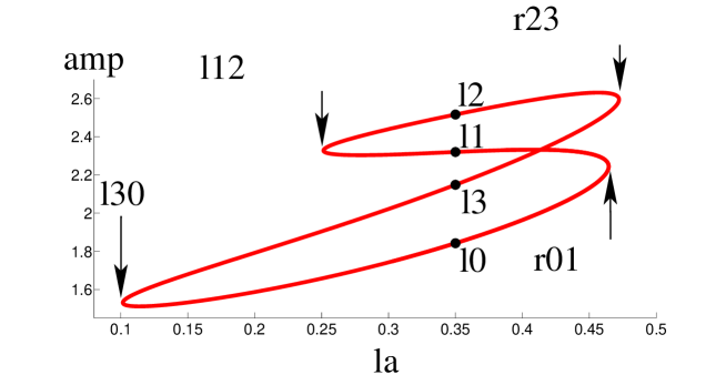
Figure 1: Continuation of homoclinic Hénon orbits. At the parameter $\tilde{\lambda}=0.35$ four distinct orbits $x_{\mathbbm{Z}}^{i}$, $i\in\{0,\dots,3\}$ exist that turn into each other via left or right turning points.

At the value $\tilde{\lambda}=0.35$ four distinct homoclinic orbits occur that we denote by $x_{\mathbbm{Z}}^{i}$, $i\in\{0,\dots,3\}$. We choose their index by following the order given by the continuation routine. The orbit $x_{\mathbbm{Z}}^{0}$ is shown in Figure 2 together with parts of the stable and the unstable manifold of the fixed point $\xi_{+}(\tilde{\lambda})$. The enlargement in this figure shows where the four orbits lie in the intersection of manifolds.

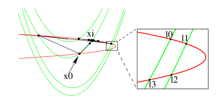
Figure 2: Primary homoclinic orbit $x_{\mathbbm{Z}}^{0}$ w.r.t. the fixed point $\xi_{+}$, and parts of the stable manifold (green) and the unstable manifold (red). The enlargement shows the intersections of manifolds that lead to the four homoclinic orbits in Figure 1.

At each turning point, two orbits collide; with $r$ and $\ell$, we distinguish right and left turning points. Figure 3 illustrates intersections of stable and unstable manifolds at these four turning points.

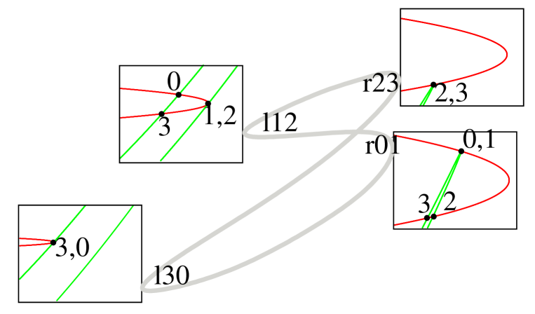
Figure 3: Intersections of stable and unstable manifolds at the four turning points in the cutout region from Figure 2.

Errors of turning point calculations for finite approximations of homoclinic orbits decay exponentially fast w.r.t. the length of the computed orbit segment, cf. [16, Theorem 5.1.1].

4 Connected components of multi-humped orbits

For Hénon’s map, we find four distinct transversal homoclinic orbits $x_{\mathbbm{Z}}^{s}$, $s\in\{0,\dots,3\}$ at $\tilde{\lambda}=0.35$ and we identify $x_{\mathbbm{Z}}(s)$ with its symbol $s$. Note that the orbits $0,1,2,3,0$ pass into each other via left (L) and right (R) turning points $r_{0,1}$, $\ell_{1,2}$, $r_{2,3}$, $\ell_{3,0}$, see Figure 3. The graph in Figure 4 gives an alternative illustration of these transitions.

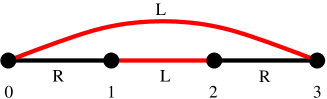
Figure 4: Transition graph for one-humped orbits.

For the construction of an $n$-humped orbit, we choose a sufficiently long interval $J=[n_{-},n_{+}]$ around zero and a sequence $s\in\mathcal{S}^{n}:=\{0,\dots,3\}^{n}$. We define the pseudo orbit

$$\tilde{x}_{\mathbbm{Z}}[s]:=x_{(-\infty,n_{+}]}^{s_{1}}x_{J}^{s_{2}}\dots x_{J}^{s_{n-1}}x_{[n_{-},\infty)}^{s_{n}},$$ (25)

see Figure 5. Since the collection of single orbits $x_{\mathbbm{Z}}^{r}$, $r\in\{0,\dots,3\}$ forms a hyperbolic set, the Shadowing-Lemma, cf. [23, 21] shows that the pseudo orbit $\tilde{x}_{\mathbbm{Z}}(s)$ lies close to a true $n$-humped $f$-orbit which we denote by $x_{\mathbbm{Z}}(s)$. In $\mathcal{S}^{n}$ there are $4^{n}$ different symbols and thus we expect to find $4^{n}$ different $n$-humped orbits $x_{\mathbbm{Z}}(s)$. We identify these orbits with their symbol.

Note that the construction of pseudo orbits in (25) slightly differs from (12), where we add up shifted orbits. With both approaches, we expect to find the same shadowing orbit for sufficiently large intervals $J$.

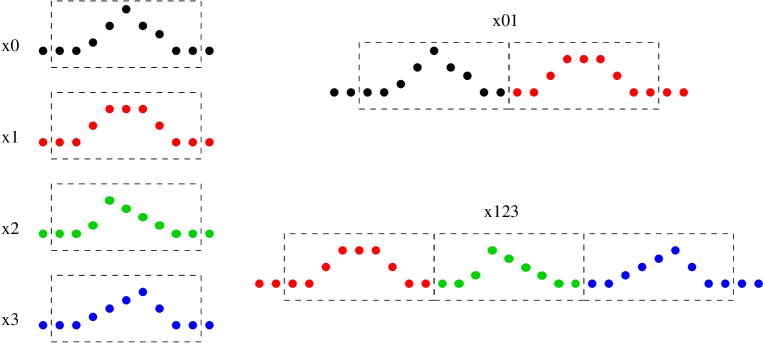
Figure 5: Construction of multi-humped orbits.

Given two symbols $s,\bar{s}\in\mathcal{S}^{n}$, we analyze whether the $n$-humped orbits $x_{\mathbbm{Z}}(s)$ and $x_{\mathbbm{Z}}(\bar{s})$ can turn into each other via continuation.

Let us first look at the two-humped case.

4.1 Bifurcation of two-humped orbits

The continuation of two-humped orbits exhibits three closed curves of homoclinic orbits, cf. Figure 6, and at the parameter value $\tilde{\lambda}$, $16$ different homoclinic orbits $x_{\mathbbm{Z}}(s)$, $s\in\mathcal{S}^{2}$ exist.

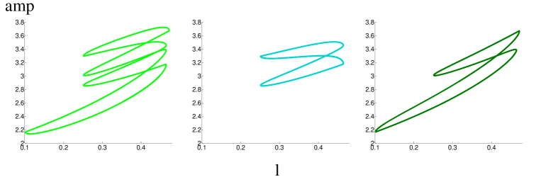
Figure 6: Continuation of two-humped orbits of length $n_{-}=-20$, $n_{+}=21$.

One observes that at each turning point in Figure 6, exactly one component of the symbol changes. For example, the symbol $(1,1)$ changes at a left turning point into the symbol $(2,1)$. Due to the combination of humps with finite length, a perturbed hilltop bifurcation decides, whether $(1,1)$ bifurcates into the symbol $(2,1)$ or into $(1,2)$, see Figure 7.

For two-humped orbits, the system (24) is a set of two equations in three variables $\lambda,\tau_{1},\tau_{2}$, called the hilltop normal form, cf. [6]

$$\lambda=\tau_{1}^{2},\quad\lambda=\tau_{2}^{2}.$$ (26)

Figure 7 (left) shows the solution curves of (26) while the red curves in Figure 7 (right) indicate the generic solution picture of a perturbed equation. Here we neglect more detailed bifurcation diagrams which take into account small hysteresis effects w.r.t. the parameter $\lambda$, see [6, Ch. IX, §3] for the unfolding theory.

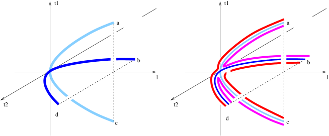
Figure 7: Unperturbed (left) and perturbed hilltop-bifurcation (right) at the turning point $\ell_{1,2}$.

4.2 Connected components and equivalent symbols

Homoclinic orbits that lie on a common closed curve define a connected component of

$$\mathcal{H}:=\big{\{}(y_{\mathbbm{Z}},\lambda)\in\ell^{\infty}(\mathbbm{R}^{k})\times\mathbbm{R}:y_{n+1}=f(y_{n},\lambda)\ \forall n\in\mathbbm{Z},\lim_{n\to\pm\infty}y_{n}=\xi(\lambda)\big{\}}.$$

More precisely, let $s\in\mathcal{S}^{n}$ and denote by $C(s)\subset\mathcal{H}$ the connected component that satisfies $(x_{\mathbbm{Z}}(s),\tilde{\lambda})\in C(s)$.

Then, we obtain an equivalence relation by identifying two sequences $s,\bar{s}\in\mathcal{S}^{n}$, if the corresponding orbits lie in the same component i.e.

$$s\cong\bar{s}\quad\Leftrightarrow\quad(x_{\mathbbm{Z}}(\bar{s}),\tilde{\lambda})\in C(s).$$ (27)

In the following, we discuss how to find these equivalence classes. Particularly, we show under some generic assumptions that each equivalence class has at least four elements, and for $n$-humped orbits it turns out that one class has at least $4n$ elements.

For this task, we introduce a labeled graph $G$ with vertices $s\in\mathcal{S}^{n}$. Two vertices $s$ and $\bar{s}\in\mathcal{S}^{n}$ are connected with an $L$ or $R$-edge, if $x_{\mathbbm{Z}}(s)$ bifurcates into $x_{\mathbbm{Z}}(\bar{s})$ via a left or right turning point. Since we do not know the effect of the perturbed hilltop bifurcation a priori, we put an edge, if the transition is possible for at least one perturbation. For example, the vertices $(1,1)$ and $(2,1)$ as well as $(1,1)$ and $(1,2)$ are connected with $L$-edges in case $n=2$, see Section 4.1. Precise rules for constructing this graph are stated in Section 4.3.

Our hypothesis is that the desired equivalence classes correspond to a special decomposition of this graph into disjoint $LR$-cycles.

In case of one-humped orbits, the only $LR$-cycle is $01230$, see Figure 4. Consequently, all symbols lie in the same equivalence class, which matches the fact that all one-humped orbits lie on the same closed curve and thus, in the same connected component of $\mathcal{H}$.

4.3 Graph structure of homoclinic network

In this section, we give precise rules for defining the labeled graph $G$ which we identify with its adjacency tensor with entries $R$ and $L$.

First, we assume that only one of the $n$ humps can turn into a neighboring hump at a turning point.

• There is no edge from $s\in\mathcal{S}^{n}$ to $\bar{s}\in\mathcal{S}^{n}$ if

  $$s=\bar{s}\quad\text{or}\quad\|s-\bar{s}\|_{1}=\sum_{i=1}^{n}d(s_{i},\bar{s}_{i})\geq 2,$$

  where $d$ is the distance on the cycle $01230$.

Now let $s,\bar{s}\in\mathcal{S}^{n}$ and assume $\|s-\bar{s}\|_{1}=1$, then there exists a unique $j$ such that $s_{j}\neq\bar{s}_{j}$.

From $\lambda^{2,3}>\lambda^{0,1}$ we conclude that the right transition at $r_{2,3}$ can only occur if the orbit contains no $0$ and no $1$ hump. Therefore, we define $R$-edges in $G$ according to the following rule.

• $G(s,\bar{s})=R$ if

  • $\{s_{j},\bar{s}_{j}\}=\{0,1\}$,

  • $\{s_{j},\bar{s}_{j}\}=\{2,3\}$ and $s_{i}\in\{2,3\}$ for all $i=1,\dots,n$.

Similarly from $\lambda^{1,2}>\lambda^{3,0}$ we conclude that the left transition at $\ell_{3,0}$ can only occur if the orbit contains no $1$ and no $2$ hump. Our rules for $L$-edges are:

• $G(s,\bar{s})=L$ if

  • $\{s_{j},\bar{s}_{j}\}=\{1,2\}$,

  • $\{s_{j},\bar{s}_{j}\}=\{0,3\}$ and $s_{i}\in\{0,3\}$ for all $i=1,\dots,n$.

We expect a connected component to correspond to an $LR$-cycle in this graph, i.e. a cycle on which $L$ and $R$-edges alternate. A precise statement of our hypothesis is as follows.

Hypothesis 7

The connected components of $n$-humped orbits and thus the equivalence classes (27) are in one to one correspondence to a partition of $G$ into disjoint $LR$-cycles.

In case $n=2$, the $L$ and $R$-edges are shown in the left and center picture of Figure 8. The right diagram additionally shows the $LR$-cycles that correspond to the connected components from Figure 6.

Similar diagrams for $n=3$ are shown in Figure 9.

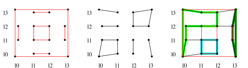
Figure 8: $L$-edges of $G$ (left) and $R$-edges (center) for two-humped orbits. The cycles in the right figure correspond to the closed curves that are computed numerically in Figure 6.

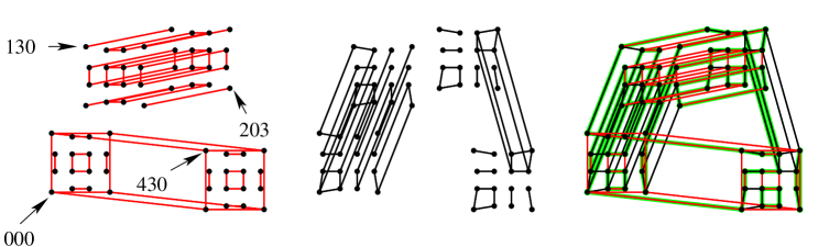
Figure 9: $L$-edges of $G$ (left) and $R$-edges (center) for three-humped orbits. The green lines in the right figure show the cycles that are computed numerically.

We continued $n$-humped orbits numerically for Hénon’s map up to $n=5$. Table 1 summarizes the number of cycles and their lengths found in the computation.

	length of cycle
$n$	4	8	12	16	20
1	1
2	2	1
3	9	2	1
4	45	3	3	1
5	205	6	6	4	1

Table 1: Continuation of $n$-humped orbits – length of occurring cycles in numerical experiments.

These experiments for $n$-humped orbits of Hénon’s map suggest that the length of occurring cycles is a multiple of $4$. Furthermore one cycle exists of at least length $4n$.

Theorem 8

Fix $n\in\mathbbm{N}$ and assume that Hypothesis 7 holds true. Then, all $n$-humped orbits lie on cycles whose length is a multiple of $4$.

For the specific symbols $s^{0}=(0,\dots,0)$ and $s^{2}=(2,\dots,2)\in\mathcal{S}^{n}$, the corresponding orbits $x_{\mathbbm{Z}}(s^{0})$ and $x_{\mathbbm{Z}}(s^{2})$ lie on a common cycle of at least length $4n$.

Remark 9

Table 1 shows that there is exactly one orbit of length $4n$ and all other orbits are shorter. Hence, the orbit of length $4n$ contains $s^{0}$ and $s^{2}$.

Proof.

By assuming Hypothesis 7 we see that it suffices to analyze $LR$-cycles of the graph $G$. More precisely, we prove Theorem 8 along the following steps.

• Each $LR$-cycle in $G$ has length $4m$, $m\geq 1$, $m\in\mathbbm{N}$.

• There exists an $LR$-cycle from $s^{0}$ to $s^{2}$ of length $4n$ and each $LR$-cycle that contains $s^{0}$ and $s^{2}$ has at least length $4n$.

• Each $LR$-cycle that contains $s^{0}$ also contains $s^{2}$.

• Let the vertices $v^{1},\dots,v^{m},v^{m+1}=v^{1}$ form an $LR$-cycle in $G$. Fix $j\in\{1,\dots,n\}$ and let $l_{j}=\#\big{\{}i\in\{1,\dots,m\}:v^{i}_{j}\neq v^{i+1}_{j},\ G(v^{i},v^{i+1})=L\big{\}}$ be the number of $L$-edges for which the corresponding vertices only differ in the $j$th component.

  From R1 it follows that $l_{j}$ is an even number and $\max_{j=1,\dots,n}\{l_{j}\}\geq 2$, otherwise the cycle cannot be closed in the $j$th component. Furthermore, an $LR$-cycle has the same number of $L$ and $R$-edges. Thus, the cycle has length

  $$m=\sum_{i=1}^{n}2l_{i}=4\sum_{i=1}^{n}\frac{l_{i}}{2}=4p\quad\text{with}\quad p=\sum_{i=1}^{n}\frac{l_{i}}{2}\geq 1.$$

• We explicitly construct an $LR$-cycle in $G$ from $s^{0}$ to $s^{2}$: $(0\cdots 0)\mapsto(10\cdots 0)$ $\mapsto(20\cdots 0)\mapsto(210\cdots 0)\mapsto(220\cdots 0)\mapsto\cdots\mapsto(2\cdots 2)\mapsto(32\cdots 2)\mapsto(312\cdots 2)\mapsto(302\cdots 2)\mapsto(3012\cdots 2)\mapsto(3002\cdots 2)\mapsto(30\cdots 0)\mapsto(0\cdots 0)$ which has length $4n$. Note that the distance from $s^{0}$ to $s^{2}$ on the full quadratic grid is $2n$ and consequently, each cycle containing these two points has at least length $4n$.

• For proving that each $LR$-cycle with $s^{0}$ also contains $s^{2}$, assume that an $LR$-cycle exists that contains $s^{2}$ but not $s^{0}$. This cycle lies in the subgraph that we obtain by deleting the vertex $s^{0}$ with its corresponding edges.

  Note that the $LR$-cycles start with an $L$ and end with an $R$-edge, and it follows from R2 that all $R$-edges that start at $s^{2}$ end in

  $$V_{3}:=\{s\in\mathcal{S}^{n}:\ \exists j\in\{1,\dots,n\}:\ s_{j}=3\}.$$

  We define the graph $\tilde{G}$ by deleting the $R$-edges of $s^{2}$ from the remaining graph. Figure 10 illustrates this construction in case $n=2$.

  

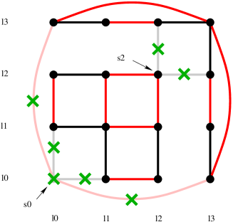
  Figure 10: Transition graph in case $n=2$. $L$-edges and $R$-edges are plotted in red and black, respectively. Vertices and edges that are deleted in the proof of Theorem 8 are marked by green crosses.

  If $\tilde{G}$ breaks into two components $V_{3}$ and $\tilde{G}\setminus V_{3}$, then we get a contradiction to the above assumption and an $LR$-cycle in the original graph $G$ that contains $s^{2}$ but not $s^{0}$ cannot exist.

  To finish the proof, we show that an $LR$-path in $\tilde{G}$ from $s^{2}$ to $V_{3}$ does not exist.

  From $s^{2}$ we cannot go directly via an $R$-edge to $V_{3}$, since the corresponding edges are deleted in $\tilde{G}$. Thus without loss of generality, we get: $(2\cdots 2)\mapsto(12\cdots 2)\mapsto(02\cdots 2)$. Denote by $v^{m}$ the $m$th vertex on this path. A $3$-component can only be achieved by the left transition $\ell_{3,0}$ or by the right transition $r_{2,3}$, see R2 and R3.

  If a $j$ exists with $v^{m}_{j}\in\{0,1\}$, then the $r_{2,3}$ transition is impossible by R2.

  If a $j$ exists with $v^{m}_{j}\in\{1,2\}$, then the $\ell_{3,0}$ transition is impossible by R3.

  Thus, we only obtain a $3$ component via the vertex $s^{0}=(0\dots 0)$ which is deleted in $\tilde{G}$.

∎

5 Bifurcation analysis near homoclinic tangencies

In this section we prove the main Theorem 1 and Theorem 5(i) by using an existence and uniqueness result for a suitable operator equation in spaces of bounded sequences. In the following we use the notation $B_{\rho}(x)$ and $B_{\rho}=B_{\rho}(0)$ to denote closed balls of radius $\rho$ in some Banach space.

5.1 The operator equation

First recall the operator $F:\ell^{\infty}(\mathbbm{R}^{k})\times\mathbbm{R}\to\ell^{\infty}(\mathbbm{R}^{k})$ from (20) and the normalization $\bar{\lambda}=0$ and $\xi(\lambda)=0$ for $\lambda$ close to $\bar{\lambda}$, see A2, A3 in Section 2. Then for any $s\in\Omega_{N}$ define the operator

$$G_{s}:\ell^{\infty}(\mathbbm{R}^{k})\times\ell^{\infty}(s)\times\ell^{\infty}(s)\times\mathbbm{R}\to\ell^{\infty}(\mathbbm{R}^{k})\times\ell^{\infty}(s)$$

by

$$G_{s}(x_{\mathbbm{Z}},g,\tau,\lambda)=\begin{pmatrix}F(p_{\mathbbm{Z}}(s)+x_{\mathbbm{Z}}+v_{\mathbbm{Z}}(s,\tau),\lambda)+w(s,g)\\ \langle\beta^{-\ell}u_{\mathbbm{Z}},x_{\mathbbm{Z}}\rangle,\ \ell\in I(s)\end{pmatrix}.$$ (28)

Here $p_{\mathbbm{Z}}$, $v_{\mathbbm{Z}}$ are defined in (12), (14) and $w(s,g)$ is given by (recall $w_{\mathbbm{Z}}$ from (17))

$$w(s,g)=\sum_{\ell\in I(s)}g_{\ell}\beta^{-\ell}w_{\mathbbm{Z}},\quad g\in\ell^{\infty}(s).$$

Our aim is to derive the functions $x_{\mathbbm{Z},s}$, $g_{s}$ in Theorem 1 by solving

$$G_{s}(x_{\mathbbm{Z}},g,\tau,\lambda)=0$$ (29)

for $\|\tau\|_{\infty}$, $|\lambda|$ sufficiently small and for all $s\in\Omega_{N}$. More precisely, we prove in Section 6 the following Reduction Theorem.

Theorem 10

There exist constants $C_{0},\rho_{x},\rho_{g},\rho_{\tau},\rho_{\lambda}>0$ and a number $N_{0}\in\mathbbm{N}$ such that for all $N\geq N_{0}$ and for all $s\in\Omega_{N}$ the following statements hold. For all $\tau\in B_{\rho_{\tau}}$, $\lambda\in B_{\rho_{\lambda}}$ the system (29) has a unique solution

$$g=g_{s}(\tau,\lambda)\in B_{\rho_{g}}\subset\ell^{\infty}(s),\quad x_{\mathbbm{Z}}=x_{\mathbbm{Z},s}(\tau,\lambda)\in B_{\rho_{x}}\subset\ell^{\infty}(\mathbbm{R}^{k}).$$

Moreover, the following estimate is satisfied:

$$\max(\|g-\tilde{g}\|_{\infty},\|x_{\mathbbm{Z}}-\tilde{x}_{\mathbbm{Z}}\|_{\infty})\leq C_{0}\|G_{s}(x_{\mathbbm{Z}},g,\tau,\lambda)-G_{s}(\tilde{x}_{\mathbbm{Z}},\tilde{g},\tau,\lambda)\|$$ (30)

for all $g,\tilde{g}\in B_{\rho_{g}}$, $x_{\mathbbm{Z}},\tilde{x}_{\mathbbm{Z}}\in B_{\rho_{x}}$, $\tau\in B_{\rho_{\tau}}$, $\lambda\in B_{\rho_{\lambda}}$.

5.2 Preparatory Lemmata

In order to construct the neighborhoods $U$ and $\Lambda$ in Theorem 1 we need several lemmata.

Lemma 11

There exists $N_{1}\in\mathbbm{N}$, such that for all $N\geq N_{1}$, $s\in\Omega_{N}$ the linear system

$$\sum_{k\in I(s)}\langle\beta^{-\ell}u_{\mathbbm{Z}},\beta^{-k}u_{\mathbbm{Z}}\rangle\tau_{k}=r_{\ell},\quad\ell\in I(s),\ r\in\ell^{\infty}(s)$$ (31)

has a unique solution $\tau\in\ell^{\infty}(s)$ and

$$\|\tau\|_{\infty}\leq 2\|r\|_{\infty}.$$ (32)

Proof.

Rewrite (31) as fixed point equation

$$\tau=P\tau+r,\quad(P\tau)_{\ell}=-\sum_{k\in I(s),k\neq\ell}\langle\beta^{-\ell}u_{\mathbbm{Z}},\beta^{-k}u_{\mathbbm{Z}}\rangle\tau_{k}$$

and note

$$\|P\tau\|_{\infty} \leq \|\tau\|_{\infty}\sup_{\ell\in I(s)}\sum_{k\in I(s),k\neq\ell}|\langle u_{\mathbbm{Z}},\beta^{\ell-k}u_{\mathbbm{Z}}\rangle|$$

$$\leq \|\tau\|_{\infty}C\sum_{j\geq 1}{\rm{e}}^{-\alpha jN}=\frac{C{\rm{e}}^{-\alpha N}}{1-{\rm{e}}^{-\alpha N}}\|\tau\|_{\infty}.$$

Thus, we choose $N_{1}$ such that $\frac{C{\rm{e}}^{-\alpha N_{1}}}{1-{\rm{e}}^{-\alpha N_{1}}}\leq\frac{1}{2}$. Then $P$ is contractive and (32) follows. ∎

Lemma 12

There exist $N_{2}\in\mathbbm{N}$, $C_{2}>0$ such that

$$\|F(p_{\mathbbm{Z}}(s)+v_{\mathbbm{Z}}(s,\tau),\lambda)\|_{\infty}\leq C_{2}(|\lambda|+\|\tau\|_{\infty}^{2}+{\rm{e}}^{-\alpha N/2})$$ (33)

for all $N\geq N_{2}$, $s\in\Omega_{N}$, $|\lambda|\leq 1$, $\tau\in B_{1}\subset\ell^{\infty}(s)$.

Proof.

We estimate

$$p_{n+1}(s)+v_{n+1}(s,\tau)-f(p_{n}(s)+v_{n}(s,\tau),\lambda)$$

$$= \sum_{\ell\in I(s)}(\bar{x}_{n+1-\ell}+\tau_{\ell}u_{n+1-\ell})-f(p_{n}(s)+v_{n}(s,\tau),0)+\mathcal{O}(|\lambda|)$$

$$= \sum_{\ell\in I(s)}\big{(}f(\bar{x}_{n-\ell},0)+\tau_{\ell}f_{x}(\bar{x}_{n-\ell},0)u_{n-\ell}\big{)}$$

$$-f\big{(}\sum_{\ell\in I(s)}\bar{x}_{n-\ell}+\sum_{\ell\in I(s)}\tau_{\ell}u_{n-\ell},0\big{)}+\mathcal{O}(|\lambda|)$$

$$= \sum_{\ell\in I(s)}f(\bar{x}_{n-\ell},0)+\sum_{\ell\in I(s)}\tau_{\ell}f_{x}(\bar{x}_{n-\ell},0)u_{n-\ell}$$

$$-f\big{(}\sum_{\ell\in I(s)}\bar{x}_{n-\ell},0\big{)}-f_{x}\big{(}\sum_{j\in I(s)}\bar{x}_{n-j},0\big{)}\sum_{\ell\in I(s)}\tau_{\ell}u_{n-\ell}+\mathcal{O}(|\lambda|+\|\tau\|_{\infty}^{2}).$$

For $n\in\mathbbm{Z}$, choose $\tilde{\ell}\in I(s)$ such that $|n-\tilde{\ell}|\leq|n-\ell|$ for all $\ell\in I(s)$. Then $|n-\ell|\geq\frac{N}{2}$ for all $\ell\neq\tilde{\ell}$ and, therefore, by (7),

$$\Big{\|}\sum_{\ell\in I(s)}f(\bar{x}_{n-\ell},0)-f\big{(}\sum_{\ell\in I(s)}\bar{x}_{n-\ell},0\big{)}\Big{\|}$$ (34)

$$\leq \Big{\|}\sum_{\ell\in I(s),\ell\neq\tilde{\ell}}f(\bar{x}_{n-\ell},0)\Big{\|}+\Big{\|}f(\bar{x}_{n-\tilde{\ell}},0)-f\big{(}\sum_{\ell\in I(s)}\bar{x}_{n-\ell},0\big{)}\Big{\|}$$

$$\leq \Big{\|}\sum_{\ell\in I(s),\ell\neq\tilde{\ell}}\bar{x}_{n+1-\ell}\Big{\|}+L\Big{\|}\sum_{\ell\in I(s),\ell\neq\tilde{\ell}}\bar{x}_{n-\ell}\Big{\|}\leq C_{2}{\rm{e}}^{-\alpha N/2}.$$

In a similar way,

$$\sum_{\ell\in I(s)}\tau_{\ell}f_{x}\big{(}\sum_{j\in I(s)}\bar{x}_{n-j},0\big{)}u_{n-\ell}=\sum_{\ell\in I(s)}\tau_{\ell}f_{x}(\bar{x}_{n-\ell},0)u_{n-\ell}+\mathcal{O}({\rm{e}}^{-\alpha N/2}\|\tau\|_{\infty}).$$ (35)

Combining these estimates, we obtain (33). ∎

Lemma 13

Assume A1, A2 and let $\bar{x}_{\mathbbm{Z}}$ be a homoclinic $f(\cdot,0)$-orbit with respect to the hyperbolic fixed point $0$. Then, there exist zero neighborhoods $U_{3}\subset\mathbbm{R}^{k}$, $\Lambda_{3}\subset\Lambda_{0}$ and constants $N_{3},n_{0},\alpha>0,C_{3}\geq 1$ such that the following statement holds for all $K\geq N_{3}$, $-n_{-},n_{+}\geq n_{0}$:

If $x_{n+1}=f(x_{n},\lambda)$ for $n\in\tilde{J}:=[0,K-1]$, $\lambda\in\Lambda_{3}$, and if $x_{n}\in U_{3}$ for all $n\in J:=[0,K]$ then we have the estimate

$$\sup_{j\in J}\|x_{j}-\bar{x}_{n_{-}+1-K+j}-\bar{x}_{n_{+}-1+j}\|\leq C_{3}\left(\|x_{K}-\bar{x}_{n_{-}+1}\|+\|x_{0}-\bar{x}_{n_{+}-1}\|+|\lambda|+{\rm{e}}^{-\alpha\frac{K}{2}}\right).$$

Furthermore we obtain in case $K=\infty$:

$$\sup_{j\geq 0}\|x_{j}-\bar{x}_{n_{+}-1+j}\|\leq C_{3}(\|x_{0}-\bar{x}_{n_{+}-1}\|+|\lambda|).$$ (36)

Proof.

Consider the pseudo-orbit $p_{j}:=\bar{x}_{n_{+}-1+j}+\bar{x}_{n_{-}+1-K+j}$, $j\in J$ which is a zero of the boundary value operator

$$\Gamma_{J}(y_{J},\lambda):=\begin{pmatrix}y_{n+1}-f(y_{n},\lambda)-\rho_{n},\quad n\in\tilde{J}\\ b_{K}(y_{0},y_{K})\end{pmatrix},$$

at $\lambda=0$, where

$$\rho_{n} := f(\bar{x}_{n_{+}-1+n},0)+f(\bar{x}_{n_{-}+1-K+n},0)-f(p_{n},0),\quad n\in J,$$

$$b_{K}(y_{0},y_{K}) := \begin{pmatrix}P_{s}(y_{0}-p_{0})\\ P_{u}(y_{K}-p_{K})\end{pmatrix}.$$

Here $P_{s}$ and $P_{u}$ are the stable and unstable projectors of the fixed point $0$.

Let $b$ be the bound from Theorem 21 for the difference equation

$$u_{n+1}=(f_{x}(0,0)+B_{n})u_{n},\quad B_{n}=f_{x}(p_{n},\lambda)-f_{x}(0,0),\quad n\in\tilde{J}.$$

For sufficiently large $-n_{-},n_{+}\geq n_{0}$ and $\lambda\in\Lambda_{3}$ sufficiently small, we get $\|B_{n}\|\leq b$ for all $n\in\tilde{J}$. Consequently

$$u_{n+1}=f_{n}(p_{n},\lambda)u_{n},\quad n\in\tilde{J}$$

has an exponential dichotomy on $J$ with projectors $P_{n}^{s},P_{n}^{u}$ and an exponential rate $\alpha$ that is independent of $n_{-}$, $n_{+}$, $\lambda$ and $K$.

As in the proof of [12, Theorem 4], we show that for $\lambda\in\Lambda_{3}$, $n_{-},n_{+}\geq n_{0}$ and $K\geq N_{3}$ we have a uniform bound

$$\|D_{1}\Gamma_{J}(p_{J},\lambda)^{-1}\|_{\infty}\leq\sigma^{-1}.$$ (37)

In order to see this, consider the inhomogeneous difference equation

$$u_{n+1}-f_{x}(p_{n},\lambda)u_{n} = r_{n},\quad n=0,\dots K-1,$$ (38)

$$P_{s}u_{0}+P_{u}u_{K} = \gamma.$$ (39)

Denote by $\Phi$ the solution operator of the homogeneous equation and let $G$ be the corresponding Green’s function, cf. (88). The general solution of (38) is given by

$$u_{n}=\Phi(n,0)v+\sum_{m\in\tilde{J}}G(n,m+1)r_{m},$$ (40)

where

$$v=v_{-}+\Phi(0,K)v_{+},\quad v_{-}\in\mathcal{R}(P_{0}^{s}),\quad v_{+}\in\mathcal{R}(P_{K}^{u}).$$

Inserting (40) into (39), it remains to solve

$$P_{s}\big{(}v_{-}+\Phi(0,K)v_{+}\big{)}+P_{u}\big{(}\Phi(K,0)v_{-}+v_{+}\big{)}=R,$$

with

$$R=\gamma-P_{s}\sum_{m\in\tilde{J}}G(0,m+1)r_{m}-P_{u}\sum_{m\in\tilde{J}}G(K,m+1)r_{m}.$$

This finite-dimensional system has a unique solution for $K\geq N_{3}$ sufficiently large since $\|P_{s}-P_{0}^{s}\|\to 0$ and $\|P_{u}-P_{K}^{u}\|\to 0$ as $K\to\infty$. Therefore, the system (38), (39) also has a unique solution $u_{J}$ for $K$ large and the dichotomy estimates lead to a bound

$$\|u_{J}\|_{\infty}\leq\sigma^{-1}(|\gamma|+\|r_{J}\|_{\infty}),$$

i.e. (37) holds.

We apply Theorem 19 with the space $Y=\ell^{\infty}_{J}=\{(y_{n})_{n\in J}:y_{n}\in\mathbbm{R}^{k}\}$ of finite sequences and with $Z=\ell^{\infty}_{\tilde{J}}\times\mathbbm{R}^{k}$, both endowed with the sup-norm. We take $y_{0}=p_{J}$ and use uniform data for all $\lambda\in\Lambda_{3}$. For $\delta$ sufficiently small we have

$$\|D_{1}\Gamma_{J}(x_{J},\lambda)-D_{1}\Gamma_{J}(p_{J},\lambda)\|_{\infty}\leq\frac{\sigma}{2}\text{ for all sequences}\;x_{J}\in B_{\delta}(p_{J}),\lambda\in\Lambda_{3},$$

and by choosing the neighborhood $\Lambda_{3}$ sufficiently small we get

$$\|\Gamma_{J}(p_{J},\lambda)\|_{\infty} = \sup_{n\in\tilde{J}}\|p_{n+1}-f(p_{n},\lambda)-\rho_{n}\|+\|b_{K}(p_{0},p_{K})\|$$

$$= \sup_{n\in\tilde{J}}\|p_{n+1}-f(p_{n},\lambda)+f(p_{n},0)$$

$$\qquad-f(\bar{x}_{n_{+}-1+n},0)-f(\bar{x}_{n_{-}+1-K+n},0)\|$$

$$= \sup_{n\in\tilde{J}}\|f(p_{n},0)-f(p_{n},\lambda)\|\leq\frac{\sigma}{2}\delta\quad\text{for }\lambda\in\Lambda_{3}.$$

Theorem 19 applies to $\lambda\in\Lambda_{3}$ with uniform data, and it follows from (120) with some constant $C_{3}>0$ that

$$\|x_{J}-y_{J}\|_{\infty}\leq C_{3}\|\Gamma_{J}(x_{J},\lambda)-\Gamma_{J}(y_{J},\lambda)\|_{\infty}\quad\text{for all }x_{J},y_{J}\in B_{\delta}(p_{J}),\lambda\in\Lambda_{3}.$$ (41)

From (7) we find a number $n_{0}$ such that $\bar{x}_{n}\in B_{\frac{\delta}{2}}(0)$ for all $|n|\geq n_{0}$ and also $p_{n}\in B_{\frac{\delta}{2}}(0),n\in J$ for all $-n_{-},n_{+}\geq n_{0}$. Then we take $U_{3}:=B_{\frac{\delta}{2}}(0)$ as our neighborhood and note that (41) holds for any two sequences $x_{J},y_{J}$ in $U_{3}$. For $n\in\tilde{J}$ and $\lambda\in\Lambda_{3}$ it follows that

$$f(p_{n},\lambda)-p_{n+1}$$

$$= f(\bar{x}_{n_{+}-1+n}+\bar{x}_{n_{-}+1-K+n},\lambda)-\bar{x}_{n_{+}-1+n+1}-\bar{x}_{n_{-}+1-K+n+1}$$

$$= f(\bar{x}_{n_{+}-1+n}+\bar{x}_{n_{-}+1-K+n},0)-f(\bar{x}_{n_{+}-1+n},0)-f(\bar{x}_{n_{-}+1-K+n},0)+\mathcal{O}(|\lambda|)$$

$$= \left\{\begin{array}[]{ll}-f(\bar{x}_{n_{-}+1-K+n},0)+\mathcal{O}(\|\bar{x}_{n_{-}+1-K+n}\|)&\text{ for }0\leq n\leq\frac{K}{2}\\[5.69054pt] -f(\bar{x}_{n_{+}-1+n},0)+\mathcal{O}(\|\bar{x}_{n_{+}-1+n}\|)&\text{ for }\frac{K}{2}<n\leq K\end{array}\right\}+\mathcal{O}(|\lambda|)$$

$$= \mathcal{O}({\rm{e}}^{-\alpha\frac{K}{2}}+|\lambda|).$$

Now let $x_{J}$ be a sequence in $U_{3}$ such that $x_{n+1}=f(x_{n},\lambda)$ for all $n\in\tilde{J}$, and some $\lambda\in\Lambda_{3}$. Then

$$\|x_{J}-p_{J}\|_{\infty} \leq C\|\Gamma_{J}(x_{J},\lambda)-\Gamma_{J}(p_{J},\lambda)\|_{\infty}$$

$$\leq C\Big{(}\sup_{n\in\tilde{J}}\|f(p_{n},\lambda)-p_{n+1}\|+\|b_{K}(x_{0},x_{K})\|\Big{)}$$

$$\leq C\left({\rm{e}}^{-\alpha\frac{K}{2}}+|\lambda|+\left\|\begin{pmatrix}P_{s}(x_{0}-p_{0})\\ P_{u}(x_{K}-p_{K})\end{pmatrix}\right\|\right)$$

$$\leq C\left({\rm{e}}^{-\alpha\frac{K}{2}}+\|x_{0}-p_{0}\|+\|x_{K}-p_{K}\|+|\lambda|\right)$$

$$\leq C_{3}\left({\rm{e}}^{-\alpha\frac{K}{2}}+\|x_{0}-\bar{x}_{n_{+}-1}\|+\|x_{K}-\bar{x}_{n_{-}+1}\|+|\lambda|\right).$$

In case $K=\infty$, one uses the operator

$$\tilde{\Gamma}_{\mathbbm{N}}(y_{\mathbbm{N}},\lambda)=\begin{pmatrix}y_{n+1}-f(y_{n}),\quad n\in\mathbbm{N}\\ P_{s}(y_{0}-\bar{x}_{n_{+}-1})\end{pmatrix},$$

and it turns out that $D_{1}\tilde{\Gamma}_{\mathbbm{N}}(p_{\mathbbm{N}},\lambda)$ with $p_{j}=\bar{x}_{n_{+}-1+j}$ has a uniformly bounded inverse for $\lambda\in\Lambda_{3}$ and sufficiently large $-n_{-},\ n_{+}$. Then the estimate (36) follows immediately.

∎

5.3 Proof of Main Theorem

Let us first prove assertion (i) in Theorem 1.
Step 1: (Construction of neighborhoods $U,\Lambda$)
In the following $\Lambda_{1}\supset\Lambda_{2}\supset\ldots$ will denote shrinking neighborhoods of $0$. Let $\rho_{g},\rho_{x}>0$ be given by Theorem 10 and note that we can decrease $\rho_{\tau},\rho_{\lambda}$ without changing the assertion of Theorem 10. Introduce the constants (cf. (7) and Lemma 12, 13)

$$\alpha_{*}={\rm{e}}^{-\alpha},\quad C_{4}=C_{3}+\frac{2C_{e}}{1-\alpha_{*}},\quad C_{5}=C_{e}\frac{3-\alpha_{*}}{1-\alpha_{*}},\quad C_{6}=C_{0}C_{2}+\frac{2C_{e}}{1-\alpha_{*}}.$$ (43)

Let $\rho_{\tau}>0$ be such that

$$C_{5}\rho_{\tau}\leq\frac{\rho_{x}}{4}.$$ (44)

By Lemma 13 we can choose a ball $B_{3\varepsilon_{0}}\subset U_{3}$ and numbers $n_{+},-n_{-}\geq n_{0}$ such that $\bar{x}_{n}\in B_{\varepsilon_{0}}$ for all $n\geq n_{+}-1$ and $n\leq n_{-}+1$. It is well known that the only full orbit in a small neighborhood of a hyperbolic fixed point is the fixed point itself. That is, we can assume w.l.o.g. that $U_{3},\Lambda_{3}$ satisfy

$$y_{n+1}=f(y_{n},\lambda),\ y_{n}\in U_{3}(n\in\mathbbm{Z}),\ \lambda\in\Lambda_{3}\Rightarrow y_{n}=0\;\text{for all}\;n\in\mathbbm{Z}.$$ (45)

The set $\mathcal{K}=\{0\}\cup\{\bar{x}_{n}:n\leq n_{-}\;\text{or}\;n\geq n_{+}\}$ is compact and satisfies

$$f(\mathcal{K},0)\subset\mathcal{K}\cup\{\bar{x}_{n_{-}+1}\}.$$

Thus we find an $\varepsilon\leq\varepsilon_{0}$ and $\Lambda_{4}\subset\Lambda_{3}$ such that the following properties hold

$$V_{0}:=B_{\varepsilon}\cup\bigcup_{n\leq n_{-},n\geq n_{+}}B_{\varepsilon}(\bar{x}_{n})\subset B_{2\varepsilon_{0}}\subset U_{3},$$ (46)

the balls

$$B_{j}:=B_{\varepsilon}(\bar{x}_{n_{-}+j}),\ j=1,\ldots,\varkappa:=n_{+}-1-n_{-}$$ (47)

are mutually disjoint,

$$f(V_{0},\Lambda_{4})\cap B_{j}=\emptyset\quad\text{for}\quad j=2,\ldots,\varkappa,$$ (48)

$$2C_{5}(2C_{3}+1)\varepsilon\leq\frac{\rho_{\tau}}{3}\quad\text{and}\quad(2C_{3}+1)\varepsilon\leq\frac{\rho_{x}}{4},$$ (49)

see Figure 11.

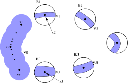
Figure 11: Construction of neighborhoods.

Next we take $N_{4}\geq\max(N_{1},N_{2},N_{3})$ (see Lemmata 11, 12, 13) such that

$$2C_{5}C_{4}{\rm{e}}^{-\alpha N_{4}}\leq\frac{\rho_{\tau}}{3},\quad C_{4}{\rm{e}}^{-\alpha N_{4}}\leq\frac{\rho_{x}}{4},\quad(2(C_{e}+C_{3})+18C_{3}C_{6}){\rm{e}}^{-\alpha N_{4}}\leq\frac{\varepsilon}{3}.$$ (50)

We can also find $\Lambda_{5}\subset\Lambda_{4}$ such that for all $\lambda\in\Lambda_{5}$

$$2C_{5}C_{3}|\lambda|\leq\frac{\rho_{\tau}}{3},\quad C_{3}|\lambda|\leq\frac{\rho_{x}}{4},\quad|\lambda|\leq\rho_{\lambda},\quad 6C_{3}|\lambda|(3C_{0}C_{2}+1)\leq\varepsilon.$$ (51)

Finally, we define

$$N=\varkappa+N_{*},\quad\text{where}\quad N_{*}=2N_{4}.$$ (52)

Then we choose $\Lambda_{6}\subset\Lambda_{5}$ such that the following settings define neighborhoods $V_{j}$ of $\bar{x}_{n_{-}+j},j=\varkappa,\ldots,1$ recursively (cf. Figure 11):

$$V_{\varkappa} =B_{\varkappa}\cap\bigcap_{n=1}^{N_{*}+1}f^{-n}(V_{0},\Lambda_{6}),$$ (53)

$$V_{j} =B_{j}\cap f^{-1}(V_{j+1},\Lambda_{6}),\quad\text{for}\quad j=\varkappa-1,\ldots,1.$$

Here we use the notation $f^{-n}(V_{j},\Lambda_{6})=\{x:f^{n}(x,\lambda)\in V_{j}\;\text{for all}\;\lambda\in\Lambda_{6}\}$.

With these settings we consider the maximal invariant set $M(U,\Lambda)$, cf. (3), that belongs to

$$U=\bigcup_{j=0}^{\varkappa}V_{j},\quad\Lambda=\Lambda_{6}.$$ (54)

Let us note that our construction (47), (48), (53), (54) implies the following three assertions for any $f(\cdot,\lambda)$-orbit $y_{\mathbbm{Z}}\subset U$, $\lambda\in\Lambda$

$$y_{n}\in V_{0},y_{n+1}\notin V_{0}\Rightarrow y_{n+1}\in V_{1},$$ (55)

$$y_{n}\in V_{j}\quad\text{for some}\quad 1\leq j\leq\varkappa-1\Rightarrow y_{n+1}\in V_{j+1},$$ (56)

$$y_{n}\in V_{\varkappa}\Rightarrow y_{n+\ell}\in V_{0}\quad\text{for}\quad\ell=1,\ldots,N_{*}+1.$$ (57)

Step 2:(Construction of symbolic sequence $s$)
For some $\lambda\in\Lambda$ consider an orbit $y_{\mathbbm{Z}}$ of (1) that lies in $U$. If it lies in $V_{0}$ then $y_{n}=0,n\in\mathbbm{Z}$ by (45) and we set $s=0\in\Omega_{N}$. Otherwise we have $y_{\tilde{n}}\notin V_{0}$ for some $\tilde{n}\in\mathbbm{Z}$. We show that

$$\tilde{I}(y_{\mathbbm{Z}}):=\{n\in\mathbbm{Z}:y_{n}\in V_{1}\}$$

is nonempty and that there is a unique $s\in\Omega_{N}$ such that $\tilde{I}(y_{\mathbbm{Z}})=I(s)$, see (9). By our assumptions we have $y_{\tilde{n}}\in V_{j_{0}}$ for some $j_{0}\in\{1,\ldots,\varkappa\}$. If $j_{0}=1$ then $\tilde{I}(y_{\mathbbm{Z}})\neq\emptyset$ whereas in case $j_{0}\geq 2$ we obtain $y_{\tilde{n}-m}\in V_{j_{0}-m},m=0,\ldots,j_{0}-1$ by induction from (56) and the fact that the $V_{j}$ are mutually disjoint. Therefore, we have $\tilde{\ell}:=\tilde{n}-j_{0}+1\in\tilde{I}(y_{\mathbbm{Z}})$. Moreover, from (55) and (57) we obtain

$$y_{\tilde{\ell}+j}\in V_{j+1},j=0,\ldots\varkappa-1,\qquad y_{\tilde{\ell}+j}\in V_{0},j=\varkappa,\ldots,\varkappa+N_{*}.$$ (58)

This shows that the difference of two consecutive indices $\tilde{\ell}<\ell$ in $\tilde{I}(y_{\mathbbm{Z}})$ is at least $N=\varkappa+N_{*}$. Therefore $\tilde{I}(y_{\mathbbm{Z}})$ belongs to $\mathbbm{Z}(N)$ (cf. (10)) and there is a unique sequence $s\in\Omega_{N}$ such that $\tilde{I}(y_{\mathbbm{Z}})=I(s)$.

The relations (58) hold whenever $\ell\in I(s)$. By (47) and (53) this gives us the estimates

$$\|y_{p+\ell+\nu}-\bar{x}_{p}\|\leq\varepsilon\quad\text{for}\quad\ell\in I(s),p=n_{-}+1,\ldots,n_{+}-1$$ (59)

for the index $\nu=-n_{-}-1$ (cf. (15)). From this we will derive the estimate

$$T_{n}:=\|y_{n+\nu}-\sum_{m\in I(s)}\bar{x}_{n-m}\|\leq C_{4}{\rm{e}}^{-\alpha N_{4}}+C_{3}|\lambda|+(2C_{3}+1)\varepsilon\quad\text{for}\quad n\in\mathbbm{Z}.$$ (60)

Consider first indices $n=p+\ell$ with $\ell\in I(s)$ and $p=n_{-}+1,\ldots,n_{+}-1$. Then with (52) we find

$$T_{n} \leq\|y_{p+\ell+\nu}-\bar{x}_{p}\|+\sum_{m\in I(s),m\neq\ell}\|\bar{x}_{p+\ell-m}\|$$ (61)

$$\leq\varepsilon+C_{e}\left(\sum_{I(s)\ni m<\ell}\alpha_{*}^{p+\ell-m}+\sum_{I(s)\ni m>\ell}\alpha_{*}^{m-\ell-p}\right)$$

$$\leq\varepsilon+C_{e}\left(\sum_{\mu\geq 1}\alpha_{*}^{\mu N+n_{-}+1}+\sum_{\mu\geq 1}\alpha_{*}^{\mu N-n_{+}+1}\right)$$

$$=\varepsilon+\frac{C_{e}}{1-\alpha_{*}^{N}}\left(\alpha_{*}^{N+n_{-}+1}+\alpha_{*}^{N-n_{+}+1}\right)$$

$$\leq\varepsilon+\frac{2C_{e}}{1-\alpha_{*}}\alpha_{*}^{N_{*}}.$$

Next consider two consecutive indices $\ell<\tilde{\ell}$ in $I(s)$ and $n=p+\ell$ for $p=n_{+}-1,\ldots,\tilde{p}=\tilde{\ell}-\ell+n_{-}+1$. For these indices we get

$$y_{n+\nu}\in\left\{\begin{array}[]{rl}V_{\varkappa},&\text{ for }p=n_{+}-1,\\ V_{1},&\text{ for }p=\tilde{p},\\ V_{0},&\text{ otherwise},\end{array}\right.$$

and we can apply Lemma 13 to this sequence in place of $\tilde{x}_{0},\ldots,\tilde{x}_{K}$, where $K=\tilde{\ell}-\ell+2-(n_{+}-n_{-})=\tilde{\ell}-\ell+1-\varkappa\geq N_{*}+1=2N_{4}+1$. With (59) this yields the estimate

$$\sup_{j=0,\ldots,K}\|y_{\ell+\nu+n_{+}-1+j}-\bar{x}_{n_{+}+j-1}-\bar{x}_{n_{-}+j-K+1}\|$$ (62)

$$\leq \ C_{3}\left(\|y_{\ell+\nu+n_{+}-1}-\bar{x}_{n_{+}-1}\|+\|y_{\ell+\nu+n_{+}-1+K}-\bar{x}_{n_{-}+1}\|+|\lambda|+\alpha_{*}^{-K/2}\right)$$

$$\leq \ C_{3}\left(2\varepsilon+|\lambda|+\alpha_{*}^{N_{4}}\right).$$

Finally, we use this to estimate for $n=p+\ell$ and $p=n_{+}-1,\ldots,\tilde{p}$

$$T_{n} \leq\|y_{n+\nu}-\bar{x}_{n-\ell}-\bar{x}_{n-\tilde{\ell}}\|+\sum_{m\in I(s),m\neq\ell,\tilde{\ell}}\|\bar{x}_{n-m}\|.$$

The first term is handled by (62). Further note that

$$\sum_{\tilde{\ell}<m\in I(s)}\|\bar{x}_{n-m}\|\ \leq C_{e}\sum_{j\geq 1}\alpha_{*}^{jN_{*}}\leq\frac{C_{e}\alpha_{*}^{N_{*}}}{1-\alpha_{*}}.$$ (63)

and the same estimate holds for $\ell>m\in I(s)$. Collecting estimates (61) to (63) we arrive at (60):

$$T_{n}\leq(2C_{3}+1)\varepsilon+C_{3}|\lambda|+C_{3}\alpha_{*}^{N_{4}}+\frac{2C_{e}}{1-\alpha_{*}}\alpha_{*}^{2N_{4}}\leq C_{4}{\rm{e}}^{-\alpha N_{4}}+C_{3}|\lambda|+(2C_{3}+1)\varepsilon.$$

Finally, we note that (60) also holds in case $\tilde{\ell}$ is the smallest index in $I(s)$ or $\ell$ is the largest index in $I(s)$, respectively. Then one repeats the previous arguments with the formal setting $\ell=-\infty$ resp. $\tilde{\ell}=\infty$ and uses the corresponding one-sided version of Lemma 13.

Step 3: (Construction and estimate of $\tau$ and $x_{\mathbbm{Z}}$)
We want to find $x_{\mathbbm{Z}}\in\ell^{\infty}(\mathbbm{R}^{k}),\tau\in\ell^{\infty}(s)$ such that (29) holds with $g=0$. The second term of the operator $G$ in (28) vanishes provided we solve

$$\sum_{m\in I(s)}\langle\beta^{-\ell}u_{\mathbbm{Z}},\beta^{-m}u_{\mathbbm{Z}}\rangle\tau_{m}=\langle\beta^{-\ell}u_{\mathbbm{Z}},\beta^{\nu}y_{\mathbbm{Z}}-p_{\mathbbm{Z}}(s)\rangle,\quad\ell\in I(s),$$ (64)

and set

$$x_{\mathbbm{Z}}=\beta^{\nu}y_{\mathbbm{Z}}-p_{\mathbbm{Z}}(s)-v_{\mathbbm{Z}}(s,\tau).$$ (65)

By Lemma 11 the linear system (64) has a unique solution $\tau\in\ell^{\infty}(s)$ which satisfies by (60), (7), (43)

$$\|\tau\|_{\infty} \leq 2\|u_{\mathbbm{Z}}\|_{\ell^{1}}\sup_{n\in\mathbbm{Z}}\|y_{n+\nu}-\sum_{m\in I(s)}\bar{x}_{n-m}\|$$

$$\leq 2C_{e}\frac{1+\alpha_{*}}{1-\alpha_{*}}\left(C_{4}{\rm{e}}^{-\alpha N_{4}}+C_{3}|\lambda|+(2C_{3}+1)\varepsilon\right).$$

Using (49), (50), (51) and $C_{e}\frac{1+\alpha_{*}}{1-\alpha_{*}}\leq C_{5}$ we end up with $\|\tau\|_{\infty}\leq\rho_{\tau}$. Next we estimate $x_{\mathbbm{Z}}$ from (65). Using (7) it is easy to show that

$$\|\sum_{\ell\in I(s)}\beta^{-\ell}u_{\mathbbm{Z}}\|_{\infty}\leq C_{e}\frac{3-\alpha_{*}}{1-\alpha_{*}}=C_{5}.$$ (66)

Therefore, when using (60) again, we find

$$\|x_{\mathbbm{Z}}\|_{\infty} \leq\|\beta^{\nu}y_{\mathbbm{Z}}-p_{\mathbbm{Z}}(s)\|_{\infty}+C_{5}\rho_{\tau}$$

$$\leq C_{4}{\rm{e}}^{-\alpha N_{4}}+C_{3}|\lambda|+(2C_{3}+1)\varepsilon+C_{5}\rho_{\tau}.$$

The estimates from (44), (49), (50), (51) then guarantee $\|x_{\mathbbm{Z}}\|_{\infty}\leq\rho_{x}$.

Therefore, we know that $G_{s}(x_{\mathbbm{Z}},0,\tau,\lambda)=0$ and the tuple $(x_{\mathbbm{Z}},0,\tau,\lambda)$ lies in the balls in which (29) has a unique solution. By uniqueness we conclude $g_{s}(\tau,\lambda)=0$ and $x_{\mathbbm{Z}}=x_{\mathbbm{Z},s}(\tau,\lambda)$ for $\lambda\in\Lambda$. Moreover, by the defining equations (64) and (65) we obtain that equality (15) holds.

Step 4: (Proof of Theorem 1 (ii))
The radius $r_{\tau}$ will be taken such that

$$18C_{3}(C_{0}C_{2}r_{\tau}^{2}+C_{5}r_{\tau})\leq\varepsilon.$$ (67)

Let $\tau\in B_{r_{\tau}}\subset\ell^{\infty}(s)$, $\lambda\in\Lambda$ satisfy $g_{s}(\tau,\lambda)=0$ for some $s\in\Omega_{N}$ and let $x_{\mathbbm{Z},s}$ be given as in Theorem 10. Then clearly, the sequence

$$y_{\mathbbm{Z}}=x_{\mathbbm{Z},s}(\tau,\lambda)+p_{\mathbbm{Z}}(s)+v_{\mathbbm{Z}}(s,\tau)$$

is an orbit of (1). It remains to show that $y_{n}\in U$ for all $n\in\mathbbm{Z}$. Application of (30) in Theorem 10 and of Lemma 12 yields the estimate

$$\|x_{\mathbbm{Z},s}(\tau,\lambda)\|_{\infty} \leq C_{0}\|G_{s}(x_{\mathbbm{Z},s}(\tau,\lambda),g_{s}(\tau,\lambda),\tau,\lambda)-G_{s}(0,0,\tau,\lambda)\|_{\infty}$$ (68)

$$=C_{0}\|F(p_{\mathbbm{Z}}(s)+v_{\mathbbm{Z}}(s,\tau),\lambda)\|_{\infty}$$

$$\leq C_{0}C_{2}(|\lambda|+\|\tau\|_{\infty}^{2}+{\rm{e}}^{-\alpha N/2}).$$

From (66) we find

$$\|v_{\mathbbm{Z}}(s,\tau)\|_{\infty}\leq C_{5}r_{\tau}.$$ (69)

We estimate the distance of $y_{\mathbbm{Z}}$ to the centers of the balls $B_{j}$ in $U$ by showing for $\nu=-n_{-}-1$

$$\|y_{p+\ell+\nu}-\bar{x}_{p}\|\leq\frac{\varepsilon}{6C_{3}}\quad\text{for}\quad p=n_{-}+1,\ldots,n_{+}-1,\ell\in I(s).$$ (70)

Note that the right-hand side is less equal $\varepsilon$ since we chose $C_{3}\geq 1$ in Lemma 13. Using (68), (69) and (61) we obtain for $\ell\in I(s)$

$$\|y_{p+\ell+\nu}-\bar{x}_{p}\| =\|x_{p+\ell,s}(\tau,\lambda)+\sum_{m\in I(s),m\neq\ell}\bar{x}_{p+\ell-m}+v_{p+\ell}(s,\tau)\|$$ (71)

$$\leq C_{0}C_{2}(|\lambda|+\|\tau\|_{\infty}^{2}+{\rm{e}}^{-\alpha N/2})+C_{5}r_{\tau}+\frac{2C_{e}}{1-\alpha_{*}}\alpha_{*}^{N_{4}}$$

$$\leq C_{0}C_{2}|\lambda|+(C_{0}C_{2}r_{\tau}+C_{5})r_{\tau}+C_{6}\alpha_{*}^{N_{4}}.$$

Conditions (50), (51) and (67) guarantee that (70) is satisfied.

Next we consider two consecutive indices $\ell<\tilde{\ell}$ in $I(s)$ and $n=p+\ell$ for $p=n_{+}-1,\ldots,\tilde{p}=\tilde{\ell}-\ell+n_{-}+1$. In the first step we show that $y_{p+\ell+\nu}\in U_{3}$. Using $p\geq n_{+}-1$ and $p+\ell-\tilde{\ell}\leq n_{-}+1$ and (63) we estimate similar to (71)

$$\|y_{p+\ell+\nu}\| \leq\|x_{p+\ell,s}(\tau,\lambda)\|+\|\bar{x}_{p}\|+\|\bar{x}_{p+\ell-\tilde{\ell}}\|+\sum_{\ell,\tilde{\ell}\neq m\in I(s)}\|\bar{x}_{p+\ell-m}\|+\|v_{p+\ell}(s,\tau)\|$$

$$\leq C_{0}C_{2}(|\lambda|+\|\tau\|_{\infty}^{2}+{\rm{e}}^{-\alpha N/2})+C_{5}r_{\tau}+\frac{2C_{e}}{1-\alpha_{*}}\alpha_{*}^{N_{4}}+2\varepsilon_{0}$$

$$\leq C_{0}C_{2}|\lambda|+(C_{0}C_{2}r_{\tau}+C_{5})r_{\tau}+C_{6}\alpha_{*}^{N_{4}}+2\varepsilon_{0}$$

$$\leq\frac{\varepsilon}{6C_{3}}+2\varepsilon_{0}\leq 3\varepsilon_{0}.$$

Since $B_{3\varepsilon_{0}}\subset U_{3}$ this proves our assertion. Now we can invoke Lemma 13 and find as in (62)

$$\sup_{j=0,\ldots,K}\|y_{\ell+\nu+n_{+}-1+j}-\bar{x}_{n_{+}+j-1}-\bar{x}_{n_{-}+j-K+1}\|\leq C_{3}\left(\frac{\varepsilon}{3C_{3}}+|\lambda|+\alpha_{*}^{N_{4}}\right).$$ (72)

For $j=0,\ldots,N_{4}$ we have $n_{-}+j-K+1\leq-N_{4}+n_{-}$ and hence

$$\|\bar{x}_{n_{-}+j-K+1}\|\leq C_{e}{\rm{e}}^{\alpha(n_{-}+N_{4}-K+1)}\leq C_{e}\alpha_{*}^{N_{4}},$$

while for $j=N_{4}+1,\ldots K$ we have $n_{+}+j-1\geq n_{+}+N_{4}$ and hence

$$\|\bar{x}_{n_{+}+j-1}\|\leq C_{e}\alpha_{*}^{n_{+}+N_{4}}\leq C_{e}\alpha_{*}^{N_{4}}.$$

Combining this with (72) we find

$$\|y_{p+\ell+\nu}-\bar{x}_{p}\| \leq\frac{\varepsilon}{3}+C_{3}|\lambda|+(C_{3}+C_{e})\alpha_{*}^{N_{4}},\quad p=n_{+}-1,\ldots,n_{+}-1+N_{4},$$

$$\|y_{p+\ell+\nu}-\bar{x}_{p-\tilde{\ell}+\ell}\| \leq\frac{\varepsilon}{3}+C_{3}|\lambda|+(C_{3}+C_{e})\alpha_{*}^{N_{4}},\quad p=n_{+}+N_{4},\ldots,\tilde{p}.$$

We have arranged the constants in (50) and (51) such that the right hand side is bounded by $\varepsilon$.

For the final step we note that we just have shown (cf. (46))

$$y_{p+\ell+\nu}\in\left\{\begin{array}[]{rl}V_{\varkappa},&\text{ for }p=n_{+}-1,\\ V_{1},&\text{ for }p=\tilde{p}=\tilde{\ell}-\ell+n_{-}+1,\\ V_{0},&\text{ for }p=n_{+},\ldots,\tilde{\ell}-\ell+n_{-}\end{array}\right.$$

for two consecutive indices $\ell<\tilde{\ell}$ in $I(s)$. On the other hand we know from (70) that $y_{p+\ell+\nu}\in B_{\varepsilon}(\bar{x}_{p}),p=n_{-}+1,\ldots,n_{+}-1$. Since $y_{\mathbbm{Z}}$ is an $f(\cdot,\lambda)$ orbit we conclude by induction from the definition (53)

$$y_{p+\ell+\nu}\in V_{p-n_{-}},\quad\text{for}\quad p=n_{+}-1,\ldots,n_{-}+1.$$

Therefore the sequence $y_{\mathbbm{Z}}$ lies in $U$ which proves our assertion.

Step 5: (Proof of Theorem 5 (i)) The proof of (21),(22) is easily accomplished by noting the equivariance relations

$$I(\beta s) =I(s)-1,\quad p_{\mathbbm{Z}}(\beta s)=\beta p_{\mathbbm{Z}}(s),\quad v_{\mathbbm{Z}}(\beta s,\beta\tau)=\beta v_{\mathbbm{Z}}(s,\tau),$$

$$w(\beta s,\beta g) =\beta w(s,g),\quad F(\beta x_{\mathbbm{Z}},\lambda)=\beta F(x_{\mathbbm{Z}},\lambda),\quad\text{and}$$

$$\langle\beta^{\ell}u_{\mathbbm{Z}},x_{\mathbbm{Z}}\rangle =\langle\beta^{\ell+1}u_{\mathbbm{Z}},\beta x_{\mathbbm{Z}}\rangle\quad\text{for}\quad\ell\in I(\beta s)=I(s)-1.$$

The assertion then follows by uniqueness from Theorem 10 since neighborhoods are shift invariant as well.

The proof of Theorem 5(ii) will be deferred to the next section.

6 Proof of Reduction Theorem

6.1 Nonlinear estimates

According to (28) the Frechet derivative of $G_{s}$ w.r.t. $x_{\mathbbm{Z}},g$ is given by

$$D_{(x,g)}G_{s}(x_{\mathbbm{Z}},g,\tau,\lambda)(y_{\mathbbm{Z}},h)= \begin{pmatrix}D_{x}F(p_{\mathbbm{Z}}(s)+x_{\mathbbm{Z}}+v_{\mathbbm{Z}}(s,\tau),\lambda)y_{\mathbbm{Z}}+w(s,h)\\ \langle\beta^{-\ell}u_{\mathbbm{Z}},y_{\mathbbm{Z}}\rangle,\;\ell\in I(s)\end{pmatrix},$$ (73)

$$D_{x}F(x_{\mathbbm{Z}},\lambda)y_{\mathbbm{Z}}= (y_{n+1}-f_{x}(x_{n},\lambda)y_{n})_{n\in\mathbbm{Z}}.$$

The key step in the proof of Theorem 10 will be a uniform bound for the inverse of $D_{(x,g)}G_{s}(0,0,0,0)$.

Lemma 14

There exist constants $\hat{C},\hat{N}>0$ such that for all $N\geq\hat{N}$, $s\in\Omega_{N}$ the operator $D_{(x,g)}G_{s}(0,0,0,0)$ is invertible and satisfies

$$\|y_{\mathbbm{Z}}\|_{\infty}+\|h\|_{\infty}\leq\hat{C}\|D_{(x,g)}G_{s}(0,0,0,0)(y_{\mathbbm{Z}},h)\|,\quad y_{\mathbbm{Z}}\in\ell^{\infty}(\mathbbm{R}^{k}),h\in\ell^{\infty}(s).$$

Before proving Lemma 14 we finish the proof of Theorem 10.

Proof.

Let $L_{x}$ and $L_{\lambda}$ be Lipschitz constants of the Jacobian $f_{x}(x,\lambda)$ with respect to $x$ and $\lambda$ in a compact ball that contains the homoclinic orbit in its interior. Then formula (73) and the bound (66) directly lead to the Lipschitz estimate

$$\|D_{(x,g)}G_{s}(x^{1}_{\mathbbm{Z}},g_{1},\tau_{1},\lambda_{1})-D_{(x,g)}G_{s}(x^{2}_{\mathbbm{Z}},g_{2},\tau_{2},\lambda_{2})\|$$ (74)

$$\leq \;L_{x}(\|x_{\mathbbm{Z}}^{1}-x_{\mathbbm{Z}}^{2}\|_{\infty}+C_{5}\|\tau_{1}-\tau_{2}\|_{\infty})+L_{\lambda}|\lambda_{1}-\lambda_{2}|$$

for all $x_{\mathbbm{Z}}^{1},x_{\mathbbm{Z}}^{2}\in B_{\rho_{x}}$, $g_{1},g_{2}\in\ell^{\infty}$, $\tau_{1},\tau_{2}\in B_{\rho_{\tau}}$, and $\lambda_{1},\lambda_{2}\in\Lambda_{0}$ with $\rho_{x},\rho_{\tau}$ taken sufficiently small. From Lemma 14 and Lemma 18 we obtain that the operators $D_{(x,g)}G_{s}(0,0,\tau,\lambda)$ are invertible for $\tau\in B_{\rho_{\tau}},\lambda\in B_{\rho_{\lambda}}$ provided we choose

$$N\geq\hat{N}\quad\text{and}\quad L_{x}C_{5}\rho_{\tau}+L_{\lambda}\rho_{\lambda}\leq\frac{1}{2\hat{C}}.$$

Then we have

$$\|D_{(x,g)}G_{s}(0,0,\tau,\lambda)^{-1}\|\leq 2\hat{C},\quad\tau\in B_{\rho_{\tau}},\lambda\in B_{\rho_{\lambda}}.$$

Now we apply Theorem 19 to every operator $F=G_{s}(\cdot,\cdot,\tau,\lambda)$ in the spaces $Y=Z=\ell^{\infty}(\mathbbm{R}^{k})\times\ell^{\infty}(s)$. Setting $\sigma=\frac{1}{2\hat{C}}$, $y_{0}=0$ and taking $L_{x}\rho_{x}\leq\frac{1}{4\hat{C}}$ we find that condition (117) is satisfied with $\kappa=\frac{1}{4\hat{C}}$ and $\delta=\rho_{x}$. Finally, we obtain from Lemma 12 for all $N\geq N_{2}$,

$$\|G_{s}(0,0,\tau,\lambda)\| =\|F(p_{\mathbbm{Z}}(s)+v_{\mathbbm{Z}}(s,\tau),\lambda)\|_{\infty}$$

$$\leq C_{2}(|\lambda|+\|\tau\|_{\infty}^{2}+{\rm{e}}^{-\alpha N/2})$$

$$\leq C_{2}(\rho_{\lambda}+\rho_{\tau}^{2}+{\rm{e}}^{-\alpha N/2}).$$

Now we select $N_{0}\geq\max(\hat{N},N_{2})$ and $\rho_{\lambda},\rho_{\tau}$ such that $C_{2}(\rho_{\lambda}+\rho_{\tau}^{2}+{\rm{e}}^{-\alpha N_{0}})\leq\frac{\rho_{x}}{4\hat{C}}$. Then we find $\|G_{s}(0,0,\tau,\lambda)\|\leq(\sigma-\kappa)\delta=\frac{\rho_{x}}{4\hat{C}},$ for all $N\geq N_{0}$, i.e. condition (118) is satisfied. An application of Theorem 19 finishes the proof. ∎

Remark 15

If instead of Theorem 19 we use a Lipschitz inverse mapping theorem with smooth parameters (cf. [13, Appendix]) then it is easily seen that the solutions $g_{s},x_{\mathbbm{Z},s}$ are smooth functions of $\tau$ and $\lambda$.

Proof.

(Theorem 5 (ii))
With $c_{\lambda},c_{x}$ from (19) define $h=h(\tau,\lambda)\in\ell^{\infty}(s)$ by

$$h_{\ell}=c_{\lambda}\lambda+c_{x}\tau_{\ell}^{2},\quad\ell\in I(s).$$

The idea is to construct elements $y_{\mathbbm{Z}}=y_{\mathbbm{Z}}(\tau,\lambda)\in\ell^{\infty}(\mathbbm{R}^{k})$ and $\gamma=\gamma(\tau,\lambda)\in\ell^{\infty}(s)$ such that the residual

$$G_{s}(p_{\mathbbm{Z}}(s)+y_{\mathbbm{Z}}+v_{\mathbbm{Z}}(s,\tau),h+\gamma,\tau,\lambda)$$

and $\gamma$ are of higher order than $\mathcal{O}(|\lambda|+\|\tau\|^{2}_{\infty})$. Then the assertion follows from (30) by comparing them to $x_{\mathbbm{Z},s}(\tau,\lambda),g_{s}(\tau,\lambda)$. We find $y_{\mathbbm{Z}},\gamma$ by Taylor expansion of $F$ (we abbreviate $F_{x}^{0}=F_{x}(p_{\mathbbm{Z}}(s),0)$ etc.)

$$F (p_{\mathbbm{Z}}(s)+y_{\mathbbm{Z}}+v_{\mathbbm{Z}}(s,\tau),\lambda)=F^{0}+F_{x}^{0}(y_{\mathbbm{Z}}+v_{\mathbbm{Z}}(s,\tau))+F_{\lambda}^{0}\lambda$$

$$+ \;\frac{1}{2}F_{xx}^{0}(y_{\mathbbm{Z}}+v_{\mathbbm{Z}}(s,\tau))^{2}+F_{x,\lambda}^{0}(y_{\mathbbm{Z}}+v_{\mathbbm{Z}}(s,\tau))\lambda+\frac{1}{2}F_{\lambda\lambda}^{0}\lambda^{2}$$

$$+ \;\mathcal{O}((|\lambda|+\|\tau\|_{\infty}+\|y_{\mathbbm{Z}}\|_{\infty})^{3}).$$

From the estimates (34), (35) in the proof of Lemma 12 we have

$$\|F^{0}\|_{\infty}=\mathcal{O}({\rm{e}}^{-\alpha N/2}),\quad\|F_{x}^{0}v_{\mathbbm{Z}}(s,\tau)\|=\mathcal{O}({\rm{e}}^{-\alpha N/2}\|\tau\|_{\infty}).$$

In a similar way, using Lipschitz constants for $f_{\lambda}$ and $f_{xx}$ we find

$$(F_{\lambda}^{0})_{n}= -\sum_{\ell\in I(s)}f_{\lambda}(\bar{x}_{n-\ell},0)+\mathcal{O}({\rm{e}}^{-\alpha N/2})$$

$$(F_{xx}^{0}(v_{\mathbbm{Z}}(s,\tau))^{2})_{n}= -\sum_{\ell\in I(s)}\tau_{\ell}^{2}f_{xx}(\bar{x}_{n-\ell},0)(u_{n-\ell})^{2}+\mathcal{O}({\rm{e}}^{-\alpha N/2}\|\tau\|_{\infty}).$$

Therefore, Taylor expansion of $G_{s}$ yields

$$G_{s} (p_{\mathbbm{Z}}(s)+y_{\mathbbm{Z}}+v_{\mathbbm{Z}}(s,\tau),h+\gamma,\tau,\lambda)=D_{(x,g)}G_{s}^{0}(y_{\mathbbm{Z}},\gamma)+(\varphi_{\mathbbm{Z}},0)$$ (75)

$$+ \;\mathcal{O}({\rm{e}}^{-\alpha N/2}+\|\tau\|_{\infty}|\lambda|+\|\tau\|_{\infty}\|y_{\mathbbm{Z}}\|_{\infty}+\lambda^{2}+\|y_{\mathbbm{Z}}\|_{\infty}^{2}+\|\tau\|_{\infty}^{3}),$$

where

$$\varphi_{n}=\sum_{\ell\in I(s)}\lambda(-f_{\lambda}(\bar{x}_{n-\ell},0)+c_{\lambda}w_{n-\ell})+\tau_{\ell}^{2}(-\frac{1}{2}f_{xx}(\bar{x}_{n-\ell},0)(u_{n-\ell})^{2}+c_{x}w_{n-\ell}).$$

This suggests to define $(y_{\mathbbm{Z}},\gamma)$ by

$$D_{(x,g)}G_{s}^{0}(y_{\mathbbm{Z}},\gamma)=-(\varphi_{\mathbbm{Z}},0).$$ (76)

From this equation and Lemma 14 we have the estimate

$$\|y_{\mathbbm{Z}}\|_{\infty}+\|\gamma\|_{\infty}\leq\tilde{C}(|\lambda|+\|\tau\|_{\infty}^{2}).$$ (77)

Taking the inner product of the first coordinate in (76) with $\beta^{-\ell}w_{\mathbbm{Z}},\ell\in I(s)$ and using (19), (85) leads to the improved estimate

$$\|\gamma\|_{\infty}\leq\tilde{C}{\rm{e}}^{-\alpha N/2}(|\lambda|+\|\tau\|_{\infty}^{2}).$$ (78)

By (77), (76) the Taylor expansion (75) of $G_{s}$ assumes the form

$$\|G_{s}(p_{\mathbbm{Z}}(s)+y_{\mathbbm{Z}}+v_{\mathbbm{Z}}(s,\tau),h+\gamma,\tau,\lambda)\|=\mathcal{O}({\rm{e}}^{-\alpha N/2}+\|\tau\|_{\infty}|\lambda|+\lambda^{2}+\|\tau\|_{\infty}^{3}).$$ (79)

With (30) and (78) this leads us to the final result

$$\|x_{\mathbbm{Z},s}(\tau,\lambda)-y_{\mathbbm{Z}}(\tau,\lambda)\|_{\infty}+\|g_{s}(\tau,\lambda)-h(\tau,\lambda)\|_{\infty}=\mathcal{O}({\rm{e}}^{-\alpha N/2}+\|\tau\|_{\infty}|\lambda|+\lambda^{2}+\|\tau\|_{\infty}^{3}).$$

∎

6.2 Linear estimates

In this subsection we prove Lemma 14. For any two integers $n_{l}\leq n_{r}$ and for any number $a\geq 0$ consider the weight function

$$\omega_{n}=\omega_{n}(a,n_{l},n_{r})=\min\left({\rm{e}}^{a(n-n_{l})},1,{\rm{e}}^{a(n_{r}-n)}\right),\quad n\in\mathbbm{Z}.$$ (80)

Note that $\omega_{\mathbbm{Z}}$ has a constant plateau of arbitrary width with exponentially decaying tails on both sides. We also allow $n_{l}=-\infty$ and $n_{r}=\infty$ (but neither $n_{l}=n_{r}=-\infty$ nor $n_{l}=n_{r}=\infty$), in which case $\omega_{\mathbbm{Z}}$ has only one-sided decay or degenerates to the maximum norm if $n_{l}=-\infty$ and $n_{r}=\infty$. In the following we will suppress the dependence of the norm on the data $n_{l},n_{r},a$, but all our estimates will be uniform with respect to

$$-\infty\leq n_{l}\leq n_{r}\leq\infty\quad 0\leq a\leq a_{0}<\alpha,$$ (81)

where $0<a_{0}<\alpha$ is fixed. The following lemma shows that exponentially decaying kernels preserve the weight.

Lemma 16

There exists a constant $K_{0}$, depending only on $a_{0},\alpha$, such that

$$\sum_{m\in\mathbbm{Z}}{\rm{e}}^{-\alpha|n-m-1|}\omega_{m}\leq K_{0}\,\omega_{n},\quad\text{for all}\quad n\in\mathbbm{Z}$$

and for all weight functions satisfying (81).

Proof.

We consider

$$\delta_{n}=\sum_{m\in\mathbbm{Z}}\omega_{n}^{-1}{\rm{e}}^{-\alpha|n-m-1|}\omega_{m}$$

only for $n\leq n_{l}$ and leave cases $n_{l}+1\leq n\leq n_{r}$ and $n_{r}+1\leq n$ to the reader.

$$\delta_{n}= \sum_{m\leq n-1}{\rm{e}}^{a(n_{l}-n)-\alpha(n-1-m)+a(m-n_{l})}+\sum_{m=n}^{n_{l}-1}{\rm{e}}^{a(n_{l}-n)-\alpha(m+1-n)+a(m-n_{l})}$$

$$+ \sum_{m=n_{l}}^{n_{r}-1}{\rm{e}}^{a(n_{l}-n)-\alpha(m+1-n)}+\sum_{m\geq n_{r}}{\rm{e}}^{a(n_{l}-n)-\alpha(m+1-n)+a(n_{r}-m)}$$

$$= {\rm{e}}^{-a}\sum_{m\leq n-1}{\rm{e}}^{-(\alpha+a)(n-1-m)}+{\rm{e}}^{-\alpha}\sum_{m=n}^{n_{l}-1}{\rm{e}}^{-(\alpha-a)(m-n)}$$

$$+ {\rm{e}}^{-(\alpha-a)(n_{l}-n)-\alpha}\sum_{m=n_{l}}^{n_{r}-1}{\rm{e}}^{-\alpha(m-n_{l})}+{\rm{e}}^{-(\alpha-a)(n_{l}-n)+\alpha(n_{l}-n_{r}-1)}\sum_{m\geq n_{r}}{\rm{e}}^{-(\alpha+a)(m-n_{r})}$$

$$\leq \frac{{\rm{e}}^{-a}+{\rm{e}}^{-\alpha}}{1-{\rm{e}}^{-(\alpha+a)}}+{\rm{e}}^{-\alpha}\left(\frac{1}{1-{\rm{e}}^{-(\alpha-a)}}+\frac{1}{1-{\rm{e}}^{-\alpha}}\right).$$

A suitable constant for all cases is $K_{0}=2\frac{1+{\rm{e}}^{-\alpha}}{1-{\rm{e}}^{-\alpha}}+{\rm{e}}^{a_{0}}+\frac{{\rm{e}}^{a_{0}}}{1-{\rm{e}}^{-(\alpha-a_{0})}}$. ∎

With the weights from above we consider the Banach space

$$\ell_{\omega}^{\infty}=\{y_{\mathbbm{Z}}\in(\mathbbm{R}^{k})^{\mathbbm{Z}}:\|y_{\mathbbm{Z}}\|_{\omega}=\sup_{n\in\mathbbm{Z}}\|y_{n}\omega_{n}^{-1}\|<\infty\}.$$

Taking the exponent $\alpha$ from (7), (18) we have the following result for the variational equation (6).

Lemma 17

Let conditions A1 - A3 and B4 hold. Then the linear system

$$y_{n+1}-f_{x}(\bar{x}_{n},0)y_{n}+hw_{n} =r_{n},\quad n\in\mathbbm{Z}$$ (82)

$$\langle u_{\mathbbm{Z}},y_{\mathbbm{Z}}\rangle =\gamma$$

has a unique solution $(y_{\mathbbm{Z}},h)\in\ell_{\omega}^{\infty}\times\mathbbm{R}$ for every $(r_{\mathbbm{Z}},\gamma)\in\ell_{\omega}^{\infty}\times\mathbbm{R}$. Moreover there is a constant $C^{*}$ such that for all weights (80) with (81),

$$\|y_{\mathbbm{Z}}\|_{\omega}+|h|\leq C^{*}(\|r_{\mathbbm{Z}}\|_{\omega}+|\gamma|\|u_{\mathbbm{Z}}\|_{\omega}).$$ (83)

If $n_{l}\leq 0\leq n_{r}$, then (83) simplifies to

$$\|y_{\mathbbm{Z}}\|_{\omega}+|h|\leq C^{*}\left(\|r_{\mathbbm{Z}}\|_{\omega}+|\gamma|\right).$$

Proof.

Let us abbreviate $A_{n}=f_{x}(\bar{x}_{n},0)$, $\mathcal{L}y_{\mathbbm{Z}}=(y_{n+1}-A_{n}y_{n})_{n\in\mathbbm{Z}}$ and denote by $\Phi$ the solution operator (122) of (121). From [22, Section 2] (see also [15]) we obtain the following facts. Equation (121) has an exponential dichotomy for $n\geq 0$ with data $(K,\alpha,P_{n}^{+s},P_{n}^{+u})$ and for $n\leq 0$ with data $(K,\alpha,P_{n}^{-s},P_{n}^{-u})$ (see Definition 20). Due to B4 we have $\mathcal{R}(P_{0}^{+s})\cap\mathcal{R}(P_{0}^{-u})=\mathrm{span}\{u_{0}\}=:Y_{0}$ and there exist decompositions

$$\mathcal{R}(P_{0}^{+s})=Y_{0}\oplus Y_{+},\quad\mathcal{R}(P_{0}^{-u})=Y_{0}\oplus Y_{-},\quad Y_{+}\cap Y_{-}=\{0\},$$ (84)

where

$$k_{s} =\mathrm{rank}(P_{n}^{+s})=\dim(Y_{+})+1,\quad(n\geq 0),$$

$$k_{u} =\mathrm{rank}(P_{n}^{-u})=\dim(Y_{-})+1,\quad(n\leq 0),$$

$$k_{u} =k-k_{s},\quad P_{n}^{+s}+P_{n}^{+u}=I\,(n\geq 0),\;P_{n}^{-s}+P_{n}^{-u}=I\,(n\leq 0).$$

The operator $\mathcal{L}:\ell^{\infty}(\mathbbm{R}^{k})\rightarrow\ell^{\infty}(\mathbbm{R}^{k})$ is Fredholm of index $0$ with

$$\mathcal{N}(\mathcal{L})={\rm{span}}\{u_{\mathbbm{Z}}\},\quad\mathcal{R}(\mathcal{L})=\{r_{\mathbbm{Z}}\in\ell^{\infty}(\mathbbm{R}^{k}):\langle w_{\mathbbm{Z}},r_{\mathbbm{Z}}\rangle=0\}.$$ (85)

One can also choose the ranges of $P_{0}^{+u}$ and $P_{0}^{-s}$ such that, in addition to (84),

$$\mathbbm{R}^{k}=Y_{0}\oplus Y_{+}\oplus Y_{-}\oplus Y_{1},\quad\mathcal{R}(P_{0}^{+u})=Y_{-}\oplus Y_{1},\quad\mathcal{R}(P_{0}^{-s})=Y_{+}\oplus Y_{1}.$$ (86)

Here $\dim Y_{1}=1$ and one can take $Y_{1}=\mathrm{span}\{w_{-1}\}$. Following [22, Lemma 2.7] the general bounded solution of $y_{n+1}-A_{n}y_{n}=r_{n},n\geq 0$ is given by

$$y^{+}_{n}=\Phi(n,0)\eta_{+}+\sum_{m\geq 0}G_{+}(n,m+1)r_{m},\quad n\geq 0,\quad\eta_{+}\in\mathcal{R}(P_{0}^{+s})$$ (87)

with the Green’s function defined as follows

$$G_{+}(n,m)=\left\{\begin{array}[]{cc}\Phi(n,m)P_{m}^{+s},&0\leq m\leq n,\\ -\Phi(n,m)P_{m}^{+u},&0\leq n<m.\end{array}\right.$$ (88)

Similarly, all bounded solutions of $y_{n+1}-A_{n}y_{n}=r_{n},n\leq-1$ are given by

$$y^{-}_{n}=\Phi(n,0)\eta_{-}+\sum_{m\leq-1}G_{-}(n,m+1)r_{m},\quad n\leq 0,\quad\eta_{-}\in\mathcal{R}(P_{0}^{-u}),$$ (89)

where

$$G_{-}(n,m)=\left\{\begin{array}[]{cc}\Phi(n,m)P_{m}^{-s},&m\leq n\leq 0,\\ -\Phi(n,m)P_{m}^{-u},&n<m\leq 0.\end{array}\right.$$ (90)

By the exponential dichotomies the Green’s functions satisfy

$$\|G_{\pm}(n,m)\|\leq K{\rm{e}}^{-\alpha|n-m|},\quad n,m\in\mathbbm{Z}_{\pm}.$$ (91)

With $u_{\mathbbm{Z}}^{T}y_{\mathbbm{Z}}:=\langle u_{\mathbbm{Z}},y_{\mathbbm{Z}}\rangle$ we may write (82) in block operator form as

$$\begin{pmatrix}\mathcal{L}&w_{\mathbbm{Z}}\\ u_{\mathbbm{Z}}^{T}&0\end{pmatrix}\begin{pmatrix}y_{\mathbbm{Z}}\\ h\end{pmatrix}=\begin{pmatrix}r_{\mathbbm{Z}}\\ \gamma\end{pmatrix}.$$ (92)

By the bordering lemma [2, Appendix] the block operator is Fredholm of the same index $0$ as $\mathcal{L}$ and, using (85), it is a linear homeomorphism in $\ell^{\infty}(\mathbbm{R}^{k})\times\mathbbm{R}$. Since $\ell_{\omega}^{\infty}$ is a closed subspace of $\ell^{\infty}(\mathbbm{R}^{k})$ it suffices to prove that the unique solution $(y_{\mathbbm{Z}},h)$ of (92) in $\ell^{\infty}(\mathbbm{R}^{k})\times\mathbbm{R}$ satisfies the estimate (83) in case $r_{\mathbbm{Z}}\in\ell_{\omega}^{\infty}$.

Take the inner product of the first equation of (82) with $w_{\mathbbm{Z}}$. Then (85) and the normalization $\|w_{\mathbbm{Z}}\|_{\ell^{2}}=1$ show $h=\langle w_{\mathbbm{Z}},r_{\mathbbm{Z}}\rangle$. Therefore, by (18),

$$|h|\leq C_{e}\|r_{\mathbbm{Z}}\|_{\omega}\sum_{n\in\mathbbm{Z}}{\rm{e}}^{-\alpha|n|}\omega_{n}\leq C_{e}\frac{1+{\rm{e}}^{-\alpha}}{1-{\rm{e}}^{-\alpha}}\|r_{\mathbbm{Z}}\|_{\omega}.$$ (93)

With this $h$ we have $z_{\mathbbm{Z}}:=r_{\mathbbm{Z}}-hw_{\mathbbm{Z}}\in\mathcal{R}(\mathcal{L})$ by (85). Below we will construct a special solution $\hat{y}_{\mathbbm{Z}}\in\ell^{\infty}(\mathbbm{R}^{k})$ of $\mathcal{L}\hat{y}_{\mathbbm{Z}}=z_{\mathbbm{Z}}$ such that for some constant $C>0$

$$\|\hat{y}_{\mathbbm{Z}}\|_{\omega}\leq C\|z_{\mathbbm{Z}}\|_{\omega}.$$ (94)

By (85) and (8) the solution of (92) is given by

$$(y_{\mathbbm{Z}},h)=(\hat{y}_{\mathbbm{Z}}+cu_{\mathbbm{Z}},h),\quad c=\gamma-\langle u_{\mathbbm{Z}},\hat{y}_{\mathbbm{Z}}\rangle,\quad h=\langle w_{\mathbbm{Z}},r_{\mathbbm{Z}}\rangle.$$ (95)

From the exponential decay (7), (18) and Lemma 16, applied to the kernel ${\rm{e}}^{-\alpha(|n|+|m|)}\leq{\rm{e}}^{\alpha}{\rm{e}}^{-\alpha|n-m-1|}$, we obtain with $C^{\prime}=C_{e}{\rm{e}}^{\alpha}K_{0}$,

$$\|\langle u_{\mathbbm{Z}},\hat{y}_{\mathbbm{Z}}\rangle u_{\mathbbm{Z}}\|_{\omega}\leq C^{\prime}\|\hat{y}_{\mathbbm{Z}}\|_{\omega},\quad\|\langle w_{\mathbbm{Z}},r_{\mathbbm{Z}}\rangle w_{\mathbbm{Z}}\|_{\omega}\leq C^{\prime}\|r_{\mathbbm{Z}}\|_{\omega}.$$

Then (93)-(95) yield the assertion

$$\|y_{\mathbbm{Z}}\|_{\omega}\leq(1+C^{\prime})\|\hat{y}_{\mathbbm{Z}}\|_{\omega}+|\gamma|\|u_{\mathbbm{Z}}\|_{\omega}\leq C(1+C^{\prime})^{2}\|r_{\mathbbm{Z}}\|_{\omega}+|\gamma|\|u_{\mathbbm{Z}}\|_{\omega}.$$

It remains to construct $\hat{y}_{\mathbbm{Z}}$ with $\mathcal{L}\hat{y}_{\mathbbm{Z}}=z_{\mathbbm{Z}}$ and (94). We determine $\eta_{+}\in\mathcal{R}(P^{+s}_{0})$ and $\eta_{-}\in\mathcal{R}(P^{-u}_{0})$ such that $\hat{y}_{n}=y^{+}_{n},n\geq 0$ with $y^{+}_{n}$ from (87), and $\hat{y}_{n}=y^{-}_{n},n\leq 0$ with $y^{-}_{n}$ from (89), and such that the definitions coincide at $n=0$. The last condition holds if and only if

$$\eta_{+}-\eta_{-}=\sum_{m\leq-1}G_{-}(0,m+1)z_{m}-\sum_{m\geq 0}G_{+}(0,m+1)z_{m}=:\Delta_{0}.$$ (96)

By (88), (90), (86) the first sum on the right is in $Y_{+}\oplus Y_{1}$ and the second sum is in $Y_{-}\oplus Y_{1}$ while the left-hand side is in $Y_{0}\oplus Y_{-}\oplus Y_{+}$. Since $z_{\mathbbm{Z}}\in\mathcal{R}(\mathcal{L})$ holds, equation (96) has a solution and thus $\Delta_{0}\in Y_{+}\oplus Y_{-}$. We conclude from (86) that $\eta_{+}=P^{+s}_{0}\Delta_{0}$ and $\eta_{-}=-P^{-u}_{0}\Delta_{0}$ are the unique solutions of (96). With (91) and Lemma 16 we estimate for $n\geq 0$

$$\|\hat{y}_{n}\|\omega_{n}^{-1}\leq K\|z_{\mathbbm{Z}}\|_{\omega}\sum_{m\geq 0}\omega_{n}^{-1}{\rm{e}}^{-\alpha|n-m-1|}\omega_{m}\leq KK_{0}\|z_{\mathbbm{Z}}\|_{\omega}.$$

An analogous estimate holds for $n\leq 0$ and this completes the proof. ∎

Proof.

(Lemma 14) We use Lemma 18 and construct an approximate right inverse $B_{+}$ of $D_{(x,g)}G_{s}^{0}=D_{(x,g)}G_{s}(0,0,0,0)$. For any $\ell\in I(s)$ we define the interval $J(\ell)=\{\ell_{-},\ldots,\ell,\ldots,\ell_{+}\}$ where right and left neighbors are given by

$$\ell_{+}=\left\{\begin{array}[]{cc}\infty,&\text{if}\quad\ell=\max I(s),\\ \ell+N_{*},&\text{otherwise},\end{array}\right.$$ (97)

$$\ell_{-}=\left\{\begin{array}[]{cc}-\infty,&\text{if}\quad\ell=\min I(s),\\ \max\{\tilde{\ell}_{+}:\tilde{\ell}\in I(s),\tilde{\ell}<\ell\}+1,&\text{otherwise}.\end{array}\right.$$ (98)

Note that the sets $J(\ell),\ell\in I(s)$ define a partitioning of $\mathbbm{Z}$. In the following we consider $N\geq\hat{N}=2N_{*}+1$ which implies $\ell-\ell_{-}\geq\ell_{+}-\ell\geq N_{*}$. During the proof $N_{*}$ will be taken sufficiently large. Given an element $(r_{\mathbbm{Z}},\gamma)\in\ell^{\infty}(\mathbbm{R}^{k})\times\ell^{\infty}(s)$, we decompose

$$r_{\mathbbm{Z}}=\sum_{\ell\in I(s)}\mathbb{1}_{J(\ell)}r_{\mathbbm{Z}},\quad\text{where}\quad(\mathbb{1}_{J(\ell)})_{n}=\left\{\begin{array}[]{cc}1,&n\in J(\ell),\\ 0,&\text{else}\end{array}\right.$$

is the characteristic function of $J(\ell)$. Let $B_{0}$ denote the solution operator of (92), then we set

$$(y^{\ell}_{\mathbbm{Z}},h_{\ell})=B_{0}(\beta^{\ell}\mathbb{1}_{J(\ell)}r_{\mathbbm{Z}},\gamma_{\ell})\quad\text{for}\quad\ell\in I(s),$$ (99)

and define $B_{+}$ as a blockwise inverse via

$$B_{+}(r_{\mathbbm{Z}},\gamma)=(y_{\mathbbm{Z}},h)=(\sum_{\ell\in I(s)}\beta^{-\ell}y^{\ell}_{\mathbbm{Z}},(h_{\ell})_{\ell\in I(s)}).$$ (100)

Using Lemma 17 with the settings $n_{l}=\ell_{-}-\ell$, $n_{r}=\ell_{+}-\ell$ we obtain a bound

$$\|y_{\mathbbm{Z}}^{\ell}\|_{\omega}+|h_{\ell}|\leq C^{*}\left(\|\beta^{\ell}\mathbb{1}_{J(\ell)}r_{\mathbbm{Z}}\|_{\omega}+|\gamma_{\ell}|\right)\leq C^{*}\left(\|r_{\mathbbm{Z}}\|_{\infty}+|\gamma_{\ell}|\right).$$ (101)

Let us abbreviate the weights from (80),

$$\omega_{n,\ell}=\omega_{n}(a,\ell_{-},\ell_{+}),\quad n\in\mathbbm{Z},\ell\in I(s).$$

Then equation (100) and (101) lead to the estimate

$$\|y_{n}\|\leq\|\sum_{\ell\in I(s)}y^{\ell}_{n-\ell}\|\leq C^{*}\left(\|r_{\mathbbm{Z}}\|_{\infty}+\|\gamma\|_{\infty}\right)\sum_{\ell\in I(s)}\omega_{n,\ell},$$

For $2{\rm{e}}^{-aN^{*}}\leq 1$ the last sum is bounded by $1+4{\rm{e}}^{-a}$ and (101) yields

$$\|B_{+}(r_{\mathbbm{Z}},\gamma)\|=\|y_{\mathbbm{Z}}\|_{\infty}+\|h\|_{\infty}\leq(2C^{*}+1+4{\rm{e}}^{-a})(\|r_{\mathbbm{Z}}\|_{\infty}+\|\gamma\|_{\infty}).$$ (102)

In the next step we show for $N^{*}$ sufficiently large,

$$\|(r_{\mathbbm{Z}},\gamma)-D_{(x,g)}G_{s}^{0}B_{+}(r_{\mathbbm{Z}},\gamma)\|\leq\frac{1}{2}(\|r_{\mathbbm{Z}}\|_{\infty}+\|\gamma\|_{\infty}),$$ (103)

which by (116), (102) gives the desired estimate

$$\|(D_{(x,g)}G_{s}^{0})^{-1}\|\leq 2(2C^{*}+1+4{\rm{e}}^{-a}).$$

We introduce $(\tilde{r}_{\mathbbm{Z}},\tilde{\gamma})=(r_{\mathbbm{Z}},\gamma)-D_{(x,g)}G_{s}^{0}(y_{\mathbbm{Z}},h)$. From (100) and the variational equation in (99) we have

$$\tilde{r}_{n}= r_{n}-\Big{(}\sum_{m\in I(s)}y_{n+1-m}^{m}-f_{x}(\sum_{p\in I(s)}\bar{x}_{n-p},0)y_{n}+\sum_{m\in I(s)}h_{m}w_{n-m}\Big{)}$$

$$= \sum_{m\in I(s)}\Big{[}f_{x}(\sum_{p\in I(s)}\bar{x}_{n-p},0)-f_{x}(\bar{x}_{n-m},0)\Big{]}y_{n-m}^{m}.$$

For $n\in\mathbbm{Z}$ there exists a unique $\ell\in I(s)$ such that $n\in J(\ell)$. Define the neighborhood $\mathcal{U}(\ell)$ of $\ell$ by $\mathcal{U}(\ell)=\{\hat{\ell},\ell,\tilde{\ell}\}$ with left neighbor $\hat{\ell}=\sup\{m\in I(s):m<\ell\}$ and right neighbor $\tilde{\ell}=\inf\{m\in I(s):m>\ell\}$ (as usual let $\hat{\ell}=-\infty$ and $\tilde{\ell}=\infty$ if the sets are empty). Using the Lipschitz constant $L_{x}$ of $f_{x}$ and (13), (101) we obtain

$$\|\tilde{r}_{n}\| \leq L_{x}\Big{(}\sum_{m\in I(s)\setminus\mathcal{U}(\ell)}\|y_{n-m}^{m}\|\sum_{m\neq p\in I(s)}\|\bar{x}_{n-p}\|+\sum_{m\in\mathcal{U}(\ell)}\|y_{n-m}^{m}\|\sum_{m\neq p\in I(s)}\|\bar{x}_{n-p}\|\Big{)}$$

$$\leq L_{x}C^{*}(\|r_{\mathbbm{Z}}\|_{\infty}+\|\gamma\|_{\infty})\Big{\{}\bar{C}\sum_{m\in I(s)\setminus\mathcal{U}(\ell)}\omega_{n,m}+\sum_{\ell\neq p\in I(s)}\|\bar{x}_{n-p}\|\Big{.}$$

$$+\Big{.}\omega_{n,\tilde{\ell}}\Big{(}\|\bar{x}_{n-\ell}\|+\sum_{p\in I(s)\setminus\{\ell,\tilde{\ell}\}}\|\bar{x}_{n-p}\|\Big{)}+\omega_{n,\hat{\ell}}\Big{(}\|\bar{x}_{n-\ell}\|+\sum_{p\in I(s)\setminus\{\ell,\hat{\ell}\}}\|\bar{x}_{n-p}\|\Big{)}\Big{\}}.$$

We show that the terms in $\{\ldots\}$ are of order $\mathcal{O}({\rm{e}}^{-aN*})$ so that the contraction estimate (103) holds for the first component if $N^{*}$ is sufficiently large. A critical term on the right-hand side is

$$\omega_{n,\tilde{\ell}}\|\bar{x}_{n-\ell}\|\leq C_{e}{\rm{e}}^{-\alpha|n-\ell|+a(n-\tilde{\ell}_{-})}\leq C_{e}{\rm{e}}^{a(\ell-\tilde{\ell}_{-})}\leq C_{e}{\rm{e}}^{-aN^{*}},\quad\ell_{-}\leq n\leq\ell_{+}.$$ (104)

The term $\omega_{n,\hat{\ell}}\|\bar{x}_{n-\ell}\|$ is handled analogously. Further,

$$\sum_{\ell\neq p\in I(s)}\|\bar{x}_{n-p}\| \leq C_{e}\Big{(}\sum_{\ell>p\in I(s)}{\rm{e}}^{-\alpha(n-p)}+\sum_{\ell<p\in I(s)}{\rm{e}}^{-\alpha(p-n)}\Big{)}$$

$$\leq C_{e}\Big{(}\sum_{\ell>p\in I(s)}{\rm{e}}^{-\alpha(\ell_{-}-p)}+\sum_{\ell<p\in I(s)}{\rm{e}}^{-\alpha(p-\ell_{+})}\Big{)}\leq 2C_{e}\frac{{\rm{e}}^{-\alpha N_{*}}}{1-{\rm{e}}^{-\alpha}}.$$

The remaining terms allow similar estimates since $n$ always lies in an exponential decaying tail of the weights and of the shifted homoclinic orbits. Finally, we use (7) and (99), (101) for $\ell\in I(s)$,

$$|\gamma_{\ell}-\langle\beta^{-\ell}u_{\mathbbm{Z}},y_{\mathbbm{Z}}\rangle| =|\sum_{n\in\mathbbm{Z}}\langle u_{n-\ell},\sum_{\ell\neq m\in I(s)}y_{n-m}^{m}\rangle|$$

$$\leq C_{e}C^{*}(\|r_{\mathbbm{Z}}\|_{\infty}+\|\gamma\|_{\infty})\sum_{n\in\mathbbm{Z}}{\rm{e}}^{-\alpha|n-\ell|}\sum_{\ell\neq m\in I(s)}\omega_{n,m}.$$

We estimate the remaining sum by using (104)

$$\sum_{n\in\mathbbm{Z}}{\rm{e}}^{-\alpha|n-\ell|}\sum_{\ell\neq m\in I(s)}\omega_{n,m} \leq\sum_{n=\ell_{-}}^{\ell_{+}}{\rm{e}}^{-\alpha|n-\ell|}\Big{(}\omega_{n,\tilde{\ell}}+\omega_{n,\hat{\ell}}+\sum_{m\in I(s)\setminus\mathcal{U}(\ell)}\omega_{n,m}\Big{)}$$

$$\quad\;+C\Big{(}\sum_{n=\ell_{+}}^{\infty}{\rm{e}}^{-\alpha(n-\ell)}+\sum_{n=-\infty}^{\ell_{-}-1}{\rm{e}}^{-\alpha(\ell-n)}\Big{)}.$$

The last two terms are $\mathcal{O}({\rm{e}}^{-\alpha N^{*}})$ since $\ell_{+}-\ell\geq N^{*}$ and $\ell-\ell_{-}\geq N^{*}$. Furthermore, we have for $\ell_{-}\leq n\leq\ell_{+}$

$$\sum_{m\in I(s)\setminus\mathcal{U}(\ell)}\omega_{n,m}\leq \sum_{\tilde{\ell}<m\in I(s)}{\rm{e}}^{a(n-m_{-})}+\sum_{\hat{\ell}>m\in I(s)}{\rm{e}}^{a(m_{+}-n)}$$

$$\leq \sum_{\tilde{\ell}<m\in I(s)}{\rm{e}}^{a(\ell_{-}-m_{-})}+\sum_{\hat{\ell}>m\in I(s)}{\rm{e}}^{a(m_{+}-\ell_{+})}\leq\frac{2{\rm{e}}^{-2aN^{*}}}{1-{\rm{e}}^{-aN^{*}}}.$$

Our final estimate is

$$\sum_{n=\ell_{-}}^{\ell_{+}}{\rm{e}}^{-\alpha|n-\ell|}\omega_{n,\tilde{\ell}} \leq\sum_{n=\ell_{-}}^{\ell}{\rm{e}}^{-\alpha(\ell-n)+a(n-\tilde{\ell}_{-})}+\sum_{n=\ell+1}^{\ell_{+}}{\rm{e}}^{-\alpha(n-\ell)+a(n-\tilde{\ell}_{-})}$$

$$\leq\frac{{\rm{e}}^{-aN^{*}}}{1-{\rm{e}}^{-\alpha}}+\frac{{\rm{e}}^{-aN^{*}}}{1-{\rm{e}}^{-(\alpha-a)}}.$$

The term $\sum_{n=\ell_{-}}^{\ell_{+}}{\rm{e}}^{-\alpha|n-\ell|}\omega_{n,\hat{\ell}}$ is estimated in a similar way. This finishes the proof of (103).

We take the same $B_{-}=B_{+}$ as an approximate left inverse in Lemma 18. It is convenient to require $0<2a\leq a_{0}<\alpha$ instead of (81). Given $(y_{\mathbbm{Z}},h)\in\ell^{\infty}(\mathbbm{R}^{k})\times\ell^{\infty}(s)$, we set

$$(\eta_{\mathbbm{Z}},t)=B_{+}D_{(x,g)}G_{s}^{0}(y_{\mathbbm{Z}},h),$$

then it is sufficient to show

$$\|\eta_{\mathbbm{Z}}-y_{\mathbbm{Z}}\|_{\infty}+\|t-h\|_{\infty}\leq\mathcal{O}({\rm{e}}^{-(\alpha-a)N_{*}})(\|y_{\mathbbm{Z}}\|_{\infty}+\|h\|_{\infty}).$$ (105)

For a fixed $\ell\in I(s)$ we consider first the case

$$y_{n}=0\quad(n\leq\ell_{-}\;\text{and}\;n>\ell_{+}),\quad h_{m}=0\quad(m\neq\ell),$$ (106)

and prove the stronger estimate (recall $\hat{N}=2N_{*}+1$)

$$\|\eta_{\mathbbm{Z}}-y_{\mathbbm{Z}}\|_{\omega}+|t_{\ell}-h_{\ell}|+\sup_{\ell\neq m\in I(s)}|t_{m}|{\rm{e}}^{\alpha(|m-\ell|-\hat{N})}\leq\mathcal{O}({\rm{e}}^{-\alpha N_{*}})(\|y_{\mathbbm{Z}}\|_{\omega}+|h_{\ell}|),$$ (107)

where $\omega_{n}=\omega_{n}(a,\ell_{-},\ell_{+})$, see (80). Then we consider the case

$$y_{n}=0\quad(n\neq\ell_{-}),\quad h=0$$ (108)

and prove the estimate

$$\|\eta_{\mathbbm{Z}}-y_{\mathbbm{Z}}\|_{\omega}+\sup_{m\in\mathbbm{Z}}|t_{m}|{\rm{e}}^{a|m-\ell_{-}|}\leq\mathcal{O}({\rm{e}}^{-aN_{*}})\|y_{\mathbbm{Z}}\|_{\omega},$$ (109)

where $\omega_{n}=\omega(a,\ell_{-},\ell_{-})$. Let us first show that the general case (105) follows from (107) and (109). With $J^{0}(\ell)=\{\ell_{-}+1,\ldots,\ell_{+}\}$, $J^{1}(\ell)=\{\ell_{-}\}$ we decompose

$$(y_{\mathbbm{Z}},h)=\sum_{m\in I(s)}\left[(\mathbb{1}_{J^{0}(m)}y_{\mathbbm{Z}},h_{m}\mathbb{1}_{\{m\}})+(\mathbb{1}_{J^{1}(m)}y_{\mathbbm{Z}},0)\right]$$

and define

$$(\eta_{\mathbbm{Z}},t)=\sum_{m\in I(s)}B_{+}D_{(x,g)}G^{0}_{s}\left[(\mathbb{1}_{J^{0}(m)}y_{\mathbbm{Z}},h_{m}\mathbb{1}_{\{m\}})+(\mathbb{1}_{J^{1}(m)}y_{\mathbbm{Z}},0)\right].$$

Similar to the proof of (103) we combine the local estimates (107) and (109),

$$\|y_{n}-\eta_{n}\| =\mathcal{O}({\rm{e}}^{-aN_{*}})\sum_{m\in I(s)}\left[\omega_{n}(a,m_{-},m_{+})(\|\mathbb{1}_{J^{0}(m)}y_{\mathbbm{Z}}\|_{\omega}+|h_{m}|)\right.$$

$$\qquad\qquad\qquad\qquad+\left.\omega_{n}(a,m_{-},m_{-})\|\mathbb{1}_{\{m_{-}\}}y_{\mathbbm{Z}}\|_{\omega}\right]$$

$$=\mathcal{O}({\rm{e}}^{-aN_{*}})(\|y_{\mathbbm{Z}}\|_{\infty}+\|h\|_{\infty})\sum_{m\in I(s)}\left[\omega_{n}(a,m_{-},m_{+})+\omega_{n}(a,m_{-},m_{-})\right].$$

$$=\mathcal{O}({\rm{e}}^{-aN_{*}})(\|y_{\mathbbm{Z}}\|_{\infty}+\|h\|_{\infty}).$$

Using the exponential weights of $t_{m}$ in (107) and (109) leads to the same estimate for $\|h-t\|_{\infty}$ and (105) is proved.

For the proof of (107) let $\gamma_{m}=\langle\beta^{-m}u_{\mathbbm{Z}},y_{\mathbbm{Z}}\rangle$ and note that (106) implies $r_{n}=0$ for $n\notin J(\ell)$. Hence $\eta_{\mathbbm{Z}}^{\ell}=\beta^{\ell}y_{\mathbbm{Z}}$ satisfies

$$\eta_{n+1}^{\ell}-f_{x}(\bar{x}_{n},0)\eta_{n}^{\ell}+h_{\ell}w_{n}=r_{n+\ell}+\left[f_{x}(p_{n+\ell}(s),0)-f_{x}(\bar{x}_{n},0)\right]\eta_{n}^{\ell}.$$

Using Lemma 17 and a Lipschitz estimate for $f_{x}$ we can compare with the solution $(y^{\ell}_{\mathbbm{Z}},t_{\ell})=B_{0}(\beta^{\ell}\mathbb{1}_{J(\ell)}r_{\mathbbm{Z}},\gamma_{\ell})$ of (99). This leads to

$$\|\beta^{-\ell}y^{\ell}_{\mathbbm{Z}}-y_{\mathbbm{Z}}\|_{\omega}+|t_{\ell}-h_{\ell}|=\mathcal{O}({\rm{e}}^{-\alpha N^{*}})(\|y_{\mathbbm{Z}}\|_{\omega}+|h_{\ell}|).$$

For the solutions $(y^{m}_{\mathbbm{Z}},t_{m})=B_{0}(\beta^{m}\mathbb{1}_{J(m)}r_{\mathbbm{Z}},\gamma_{m})=B_{0}(0,\gamma_{m})$ with $m\neq\ell$ Lemma 17 gives

$$\|\beta^{-m}y^{m}_{\mathbbm{Z}}\|_{\omega}+|t_{m}|\leq C^{*}|\gamma_{m}|\leq C_{e}\|y_{\mathbbm{Z}}\|_{\omega}\sum_{n=\ell_{-}+1}^{\ell_{+}}{\rm{e}}^{-\alpha|n-m|}=\mathcal{O}({\rm{e}}^{-\alpha(|m-\ell|-N^{*})})\|y_{\mathbbm{Z}}\|_{\omega}.$$

Collecting the last two estimates we find that $(\eta_{\mathbbm{Z}},t)=(\sum_{m\in I(s)}\beta^{-m}y^{m}_{\mathbbm{Z}},(t_{m})_{m\in I(s)})$ (cf. (100)) satisfies inequality (107).

In case condition (108) holds, let

$$r_{n}=(D_{x}F(p_{\mathbbm{Z}}(s),0)y_{\mathbbm{Z}})_{n}\;(n\in\mathbbm{Z}),\quad\gamma_{m}=\langle\beta^{-m}u_{\mathbbm{Z}},y_{\mathbbm{Z}}\rangle\;(m\in I(s)),$$

and note $r_{n}=0$ for $n\neq\ell_{-},\ell_{-}-1$ as well as

$$r_{\ell_{-}}=-f_{x}(p_{\ell_{-}}(s),0)y_{\ell_{-}},\quad r_{\ell_{-}-1}=y_{\ell_{-}}.$$ (110)

Moreover,

$$|\gamma_{m}|=|u_{\ell_{-}-m}^{T}y_{\ell_{-}}|\leq C_{e}{\rm{e}}^{-\alpha|\ell_{-}-m|}\|y_{\ell_{-}}\|,\quad m\in I(s).$$ (111)

As in (99) let $(y_{\mathbbm{Z}}^{m},t_{m})=B_{0}(\beta^{m}\mathbb{1}_{J(m)}r_{\mathbbm{Z}},\gamma_{m})$ for $m\in I(s)$. Recall $\ell_{-}-1=\hat{\ell}_{+}$ from (98) where $\hat{\ell}\in I(s)$ is the left neighbor of $\ell$. For $m\neq\ell,\hat{\ell}$ we have $y_{\mathbbm{Z}}^{m}=\beta^{-m}\gamma_{m}u_{\mathbbm{Z}}$, $t_{m}=0$ by (95) and therefore by (111),

$$\|y_{\mathbbm{Z}}^{m}\|_{\omega}\leq C_{e}^{2}\|y_{\ell_{-}}\|{\rm{e}}^{-\alpha|\ell_{-}-m|}\sup_{n\in\mathbbm{Z}}{\rm{e}}^{-\alpha|n-m|+a|n-\ell_{-}|}=\mathcal{O}({\rm{e}}^{-(\alpha-a)|\ell_{-}-m|})\|y_{\ell_{-}}\|.$$ (112)

We introduce the weights $\omega_{n}^{*}=\omega_{n}(2a,\ell_{-}-\ell,\ell_{-}-\ell)$. For $m=\ell$ we use (111) and Lemma 17 with $\omega^{*}$,

$$\|y_{\mathbbm{Z}}^{\ell}\|_{\omega^{*}}\leq C^{*}\left(\|\beta^{\ell}\mathbb{1}_{J(\ell)}r_{\mathbbm{Z}}\|_{\omega^{*}}+|\gamma_{\ell}|\|u_{\mathbbm{Z}}\|_{\omega^{*}}\right)$$ (113)

$$\leq C^{*}\left(1+C{\rm{e}}^{-(\alpha-2a)|\ell_{-}-\ell|}\right)\|y_{\ell_{-}}\|\leq C\|y_{\ell_{-}}\|.$$

In a similar manner,

$$\|y^{\hat{\ell}}_{\mathbbm{Z}}\|_{\hat{\omega}^{*}}\leq C\|y_{\ell_{-}}\|$$ (114)

holds for the weights $\hat{\omega}^{*}_{n}=\omega_{n}(2a,\hat{\ell}_{+}-\hat{\ell},\hat{\ell}_{+}-\hat{\ell})$. The $t$-values satisfy

$$|t_{\ell}| =|u_{\ell_{-}-\ell}^{T}f_{x}(p_{\ell_{-}}(s),0)y_{\ell_{-}}|\leq C{\rm{e}}^{-\alpha|\ell_{-}-\ell|}\|y_{\ell_{-}}\|,$$ (115)

$$|t_{\hat{\ell}}| =|u_{\hat{\ell}-\hat{\ell}_{+}}^{T}y_{\ell_{-}}|\leq C{\rm{e}}^{-\alpha|\hat{\ell}-\hat{\ell}_{+}|}\|y_{\ell_{-}}\|.$$

In particular, this proves the $t$-estimates in (109). Next we estimate the difference $d_{\mathbbm{Z}}=\beta^{-\ell}y_{\mathbbm{Z}}^{\ell}+\beta^{-\hat{\ell}}y_{\mathbbm{Z}}^{\hat{\ell}}-y_{\mathbbm{Z}}$ by using the exponential dichotomy on $\mathbbm{Z}$ for the constant coefficient operator $\mathcal{L}_{0}y_{\mathbbm{Z}}=(y_{n+1}-Ay_{n})_{n\in\mathbbm{Z}}$, $A=f_{x}(0,0)$. From (110) and the definition of $y_{\mathbbm{Z}}^{\ell},y_{\mathbbm{Z}}^{\hat{\ell}}$ we find

$$d_{n+1}-Ad_{n}= \;(f_{x}(\bar{x}_{n-\ell},0)-A)y_{n-\ell}^{\ell}+(f_{x}(\bar{x}_{n-\hat{\ell}},0)-A)y_{n-\hat{\ell}}^{\hat{\ell}}$$

$-t_{\mathrm{\ell }}{w}_{n-\mathrm{\ell }}-t_{\widehat{\mathrm{\ell }}}{w}_{n-\widehat{\mathrm{\ell }}}+(A-f_x($

References

- [1] E. L. Allgower and K. Georg. Numerical Continuation Methods. Springer-Verlag, Berlin, 1990. An introduction.
- [2] W.-J. Beyn. The numerical computation of connecting orbits in dynamical systems. IMA J. Numer. Anal., 10:379–405, 1990.
- [3] W.-J. Beyn, T. Hüls, J.-M. Kleinkauf, and Y. Zou. Numerical analysis of degenerate connecting orbits for maps. Internat. J. Bifur. Chaos Appl. Sci. Engrg., 14(10):3385–3407, 2004.
- [4] W.-J. Beyn and J.-M. Kleinkauf. The numerical computation of homoclinic orbits for maps. SIAM J. Numer. Anal., 34(3):1207–1236, 1997.
- [5] R. L. Devaney. An Introduction to Chaotic Dynamical Systems. Addison-Wesley Studies in Nonlinearity. Addison-Wesley Publishing Company Advanced Book Program, Redwood City, CA, second edition, 1989.
- [6] M. Golubitsky and D. G. Schaeffer. Singularities and groups in bifurcation theory. Vol. I, volume 51 of Applied Mathematical Sciences. Springer-Verlag, New York, 1985.
- [7] S. V. Gonchenko, D. V. Turaev, and L. P. Shilnikov. On the dynamic properties of diffeomorphisms with homoclinic tangencies. Sovrem. Mat. Prilozh., 7:91–117, 2003. J. Math. Sci. (N.Y.) 126, 1317-1343 (2005).
- [8] W. Govaerts. Numerical methods for bifurcations of dynamical equilibria. Society for Industrial and Applied Mathematics (SIAM), Philadelphia, PA, 2000.
- [9] J. Guckenheimer and P. Holmes. Nonlinear Oscillations, Dynamical Systems, and Bifurcations of Vector Fields, volume 42 of Applied Mathematical Sciences. Springer-Verlag, New York, 1990.
- [10] J. K. Hale and H. Koçak. Dynamics and Bifurcations, volume 3 of Texts in Applied Mathematics. Springer-Verlag, New York, 1991.
- [11] M. Hénon. A two-dimensional mapping with a strange attractor. Comm. Math. Phys., 50(1):69–77, 1976.
- [12] T. Hüls. Homoclinic trajectories of non-autonomous maps. J. Difference Equ. Appl., 17(1):9–31, 2011.
- [13] M. C. Irwin. Smooth dynamical systems, volume 17 of Advanced Series in Nonlinear Dynamics. World Scientific Publishing Co. Inc., River Edge, NJ, 2001. Reprint of the 1980 original, With a foreword by R. S. MacKay.
- [14] H. B. Keller. Numerical solution of bifurcation and nonlinear eigenvalue problems. In Applications of bifurcation theory (Proc. Advanced Sem., Univ. Wisconsin, Madison, Wis., 1976), pages 359–384. Publ. Math. Res. Center, No. 38. Academic Press, New York, 1977.
- [15] J.-M. Kleinkauf. The numerical computation and geometrical analysis of heteroclinic tangencies. Technical Report 98-048, SFB 343, 1998.
- [16] J.-M. Kleinkauf. Numerische Analyse tangentialer homokliner Orbits. PhD thesis, Universität Bielefeld, 1998. Shaker Verlag, Aachen.
- [17] J. Knobloch. Chaotic behaviour near non-transversal homoclinic points with quadratic tangency. J. Difference Equ. Appl., 12(10):1037–1056, 2006.
- [18] D. Lind and B. Marcus. An introduction to symbolic dynamics and coding. Cambridge University Press, Cambridge, 1995.
- [19] C. Mira. Chaotic dynamics. World Scientific Publishing Co., Singapore, 1987. From the one-dimensional endomorphism to the two-dimensional diffeomorphism.
- [20] J. Palis and F. Takens. Hyperbolicity and Sensitive Chaotic Dynamics at Homoclinic Bifurcations, volume 35 of Cambridge Studies in Advanced Mathematics. Cambridge University Press, Cambridge, 1993.
- [21] K. Palmer. Shadowing in dynamical systems, volume 501 of Mathematics and its Applications. Kluwer Academic Publishers, Dordrecht, 2000. Theory and applications.
- [22] K. J. Palmer. Exponential dichotomies, the shadowing lemma and transversal homoclinic points. In Dynamics reported, Vol. 1, pages 265–306. Teubner, Stuttgart, 1988.
- [23] S. Y. Pilyugin. Shadowing in Dynamical Systems, volume 1706 of Lecture Notes in Mathematics. Springer-Verlag, Berlin, 1999.
- [24] R. J. Sacker and G. R. Sell. A spectral theory for linear differential systems. J. Differential Equations, 27(3):320–358, 1978.
- [25] L. P. Šil’nikov. Existence of a countable set of periodic motions in a neighborhood of a homoclinic curve. Dokl. Akad. Nauk SSSR, 172:298–301, 1967. Soviet Math. Dokl. 8 (1967), 102–106.
- [26] S. Smale. Differentiable dynamical systems. Bull. Amer. Math. Soc., 73:747–817, 1967.