Possibility of a zero-temperature metallic phase in granular two-band superconducting films

Abstract

A variational approach is used to study the superconductor-insulator transition in two-band granular superconducting films using a resistance-shunted Josephson junction array model in this letter. We show that a zero-temperature metallic phase may exist between the superconducting and insulator phases which is absent in normal single band granular superconducting films. The metallic phase may be observable in some dirty pnictide superconductor films.

Intensive studies had been devoted to the problem of superconductor-insulator (SI) transition in low-$T_{c}$ thin films. These systems undergo phase transitions from superconductor to insulator as a function of disorder, film thickness as well as external magnetic fieldsM. P. A. Fisher (1982). The SI transition is usually modelled by a Josephson junction array model, expressed in terms of the phases of the superconductor order parameter $\theta_{i}$’s on superconducting grain $i$’s. The Hamiltonian describing the system consists of the Josephson coupling between superconducting grains $\sim J\cos(\theta_{i}-\theta_{j})$ where $(i.j)$ are nearest neighbor sites, and the charging energy $\sim{C\over 2}(\dot{\theta}_{i}-\dot{\theta}_{j})^{2}$. The system is in a superconducting phase if the Josephson term dominates, and is in the insulator phase if the charging energy dominates. It has been proposed by different authors that a dissipative term arising from coupling between superconducting grains and a dissipative metallic bath may also be important in describing the SI transition (shunted Josephson array model)Chakravarty et al. (1986, 1987); Kapitulnik et al. (2001). In particular, a zero-temperature metallic phase between superconductor and insulator phases may be stabilized by dissipation.

The physical reason behind the metallic phase is as follows: Imagine first a state dominated by charging energy. In this case the metallic bath would screen the Coulomb potential, leading to a weakening of charging energy and drives the system towards a metallic phase if the resistance is small enough ($R<R_{cI}$)asos . Alternatively, the coupling of Cooper pairs in the superconducting phase to a dissipative environment suppresses coherent tunnelling of Cooper pairs between grains owing to the Calderia-Leggett effectcaldeira-leggett and superconducting coherence is destroyed if $R>R_{cS}$. As a result a metallic phase between the superconducting and insulating phases may exist if $R_{cS}<R<R_{cI}$. The metallic phase, if exist, is a new phase of matter because of participation of incoherent boson (Cooper pairs) in low temperature transports which is absent in usual metals. Experimentally the zero-temperature metallic phase in single band superconducting films has not been found to exist so far in the absence of external magnetic fields, consistent with a theoretical finding that $R_{cI}<R_{cS}$ in single-band superconductorsNg (2001).

More recently, superconductors with more than one order parameters, i.e., the multi-band superconductorsSuhl et al. (1959) have raised attention in the physics community. Examples of multi-band superconductors include MgB₂Nagamatsu et al. (2001) and the pnictide superconductorsKamihara . It is interesting to see whether a metallic phase may exist more easily between the SI-transition in these materials. This is the purpose of this letter.

Using a variational approach, we consider in this letter the superconductor-insulator transition in two-band $s$ (and $s_{\pm}$)-wave superconducting films where the possibility of an intermediate metallic phase is investigated. We show that contrary to the case of single-band superconductors, a physically realizable condition for the zero-temperature intermediate metallic phase is found for these systems. We propose that the metallic phase may be observable in some recently discovered disordered pnictide superconductorsFW1101 .

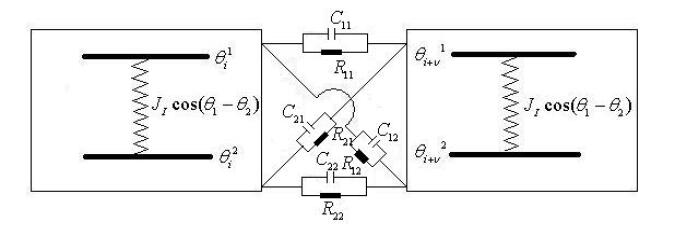
Figure 1: A qualitative sketch of our two band Josephson junction model. The two bands on different grains are connected by a capacitor, a resistor and Josephson coupling (not shown in the sketch). The two bands on the same grain are connected by in-grain inter-band Josephson coupling $J_{I}$

We start with the phase-action which is a generalization of the phase action used to study superconductor-insulator transition in one-band systemsNg (2001); Chakravarty et al. (1986, 1987). The system is schematically sketched in Fig.1. The action describes a resistance-shunted Josephson network of two-band superconductor grains and is given in imaginary time by $S=S_{\theta}+S_{\rm diss}$, where

$$S_{\theta} =\sum_{i,\nu,a,b}\int^{\beta}_{0}d\tau[{1\over 2}{C_{ab}}(\Delta_{\nu}\dot{\theta}_{i}^{ab})^{2}-J_{ab}\cos(\Delta_{\nu}\theta^{ab}_{i})]$$ (1)

$$+J_{I}\sum_{i}\int^{\beta}_{0}d\tau\cos(\theta^{1}_{i}-\theta^{2}_{i})$$

is the phase action without the dissipative term. $a,b=1,2$ represent the two different bands in a grain, and $\theta^{a}_{i}$ is the phase of band $a$ superconducting order parameter in grain $i$. $\Delta_{\nu}\theta^{ab}_{i}=\theta^{a}_{i}-\theta^{b}_{i+\nu}$ represents the phase difference between band $a$ and $b$ superconducting order parameters in neighboring grains $i$, $i+\nu$, respectively and $J_{ab}>0$ is the corresponding Josephson coupling energy. ${{1}\over{2}}C_{ab}(\Delta_{\nu}\dot{\theta}^{ab}_{i})^{2}$ represents the charging energy arising from charge imbalance between band $a$ and band $b$ electrons on grain $i$ and $i+\nu$ respectively, where $C_{ab}$ is the corresponding capacitance. $J_{I}$ is the in-grain inter-band Josephson coupling which favors $\theta^{2}_{i}=\theta^{1}_{i}+\pi$ for $J_{I}>0$, leading to a $s_{\pm}$ superconductor and favors $\theta^{1}_{i}=\theta^{2}_{i}$ for $J_{I}<0$ ($s$-wave superconductor).

$$S_{\rm diss} ={Q^{2}\over 2}\sum_{i,\nu,a,b}\int^{\beta}_{0}d\tau\int^{\beta}_{0}d\tau^{\prime}$$ (2)

$$\times\alpha_{ab}^{\rm o}(\tau-\tau^{\prime})\sin^{2}[{{D_{\nu}\theta^{ab}_{i}{(\tau)}-D_{\nu}\theta^{ab}_{i}{(\tau^{\prime})}}\over 2Q}]$$

where $\alpha_{ab}^{\rm o}(\tau)={(h/{4e^{2}R_{ab}^{\rm o}})}{[T/{\sin(\pi{T}\tau)}]^{2}}$. $R_{ab}^{\rm o}$ is the resistance between band $a$ and band $b$ electrons on grains $i$ and $i+\nu$, respectively (see Fig.(1)) and $Q=2$ is the charge of a Cooper pair. $D_{\nu}\theta_{i}^{12}=D_{\nu}\theta_{i}^{21}=[\Delta_{\nu}\theta_{i}^{11}+\Delta_{\nu}\theta_{i}^{22}]$, $D_{\nu}\theta_{i}^{aa}=[{{3}\over{2}}\Delta_{\nu}\theta_{i}^{aa}+{{1}\over{2}}\Delta_{\nu}\theta_{i}^{\bar{a}\bar{a}}]$, where $\bar{1}({\bar{2}})=2(1)$. $S_{\rm diss}$ is derived phenomenologically from a multi-band resistance network model represented by Fig.1. The details of the derivation can be found in the supplementary materials.

To simplify calculation we shall consider the grains forming a two-dimensional square lattice with $J_{12}=0$ in our following analysis. With the later condition the $s$ and $s_{\pm}$ superconductors can be transformed to each other by simply shifting $\theta^{2}_{i}\rightarrow\theta^{2}_{i}+\pi$. The main effect of $J_{12}$ is to renormalize $J_{I}\rightarrow J_{I}-zJ_{12}$ where $z$ is the lattice co-ordination number and is not going to affect our conclusion in renormalization-group sense.

Due to the compactness of the phase field ($e^{i(\theta+2n\pi)}=e^{i\theta}$), the phase variables $\theta^{a}_{i}(\tau)$ can be decomposed into a periodic part and a winding number contribution,

$$\theta^{a}_{i}(\tau)={{2\pi{n^{a}_{i}}\tau}\over{\beta}}+\theta^{a}_{i0}(\tau)$$

where $\theta^{a}_{i0}(\beta)=\theta^{a}_{i0}(0)$ and $n^{a}_{i}$ can be any arbitrary integer (winding number). With this decomposition the phase action becomes

$$S_{\theta} \rightarrow {{2\pi^{2}}\over{\beta}}\sum_{i,\nu,a,b}C_{ab}{{\Delta_{\nu}n^{ab}_{i}}^{2}}+\sum_{i,\nu,a,b}{C_{ab}\over 2}\int^{\beta}_{0}d\tau(\Delta_{\nu}\dot{\theta}^{ab}_{i0})^{2}$$ (3)

$$-\sum_{i,\nu,a}J_{aa}\int^{\beta}_{0}d\tau\cos[\Delta_{\nu}\theta^{aa}_{i0}+{2\pi\tau\over\beta}\Delta_{\nu}n^{aa}_{i}]$$

$$+J_{I}\sum_{i}\int^{\beta}_{0}d\tau\sum_{\nu}\cos[\Delta\theta_{i0}+{{2\pi\tau}\over\beta}\Delta n_{i}].$$

where $\Delta_{\nu}n^{ab}_{i}=n^{a}_{i}-n^{b}_{i+\nu}$, $\Delta\theta_{i0}=\theta^{1}_{i0}(\tau)-\theta^{2}_{i0}(\tau)$ and $\Delta n_{i}=n^{1}_{i}-n^{2}_{i}$ and

$$S_{\rm diss} \rightarrow \sum_{i,\nu,a,b}{Q\pi\over 4R_{ab}}|D_{\nu}n^{ab}_{i}|+{1\over 8}\sum_{i,\nu,a,b}\int^{\beta}_{0}d\tau\int^{\beta}_{0}d\tau^{\prime}$$ (4)

$$\alpha_{ab}^{\rm o}(\tau-\tau^{\prime})\cos[{2\pi(\tau-\tau^{\prime})\over Q\beta}D_{\nu}n^{ab}_{i}]$$

$$\times[D_{\nu}\theta^{ab}_{i0}(\tau)-D_{\nu}\theta^{ab}_{i0}(\tau^{\prime})]^{2}.$$

where $D_{\nu}n_{i}^{ab}$ is defined in the same way as $D_{\nu}\theta_{i}^{ab}$ with $\Delta_{\nu}\theta_{i}^{ab}\rightarrow\Delta_{\nu}n_{i}^{ab}=n^{a}_{i}-n^{b}_{i+\nu}$. We have assumed strong dissipation and keep only to second order terms of $\Delta_{\nu}\theta^{aa}_{0i}$ in $S_{\rm diss}$ for simplicityNg (2001).

To proceed further we employ a variational approachNg (2001). We consider a trial action $S_{\rm trial}=S^{P}_{\rm trial}+S^{n}_{\rm trial}$ where the periodic and the winding number contributions to $\theta$ are decoupled.

$$S^{P}_{\rm trial} = \sum_{i,\nu,a,b}\int^{\beta}_{0}d\tau[{C_{ab}\over 2}(\Delta_{\nu}\dot{\theta}^{ab}_{i0})^{2}+{J_{aa}^{\rm eff}\over 2}(\Delta_{\nu}\theta^{aa}_{i0})^{2}]$$ (5)

$$+{J_{I}^{\rm eff}\over 2}\sum_{i}\int^{\beta}_{0}d\tau{(\Delta\theta_{i0})^{2}}+$$

$${1\over 8}\sum_{i,\nu,a,b}\int^{\beta}_{0}d\tau\int^{\beta}_{0}d\tau^{\prime}\alpha^{\rm{eff},o}_{ab}(\tau-\tau^{\prime})\times$$

$${[D_{\nu}\theta^{ab}_{i0}(\tau)-D_{\nu}\theta^{ab}_{i0}(\tau^{\prime})]^{2}}$$

is an effective action describing Gaussian fluctuations of the periodic phases around the saddle point $\theta^{1}_{i0}(\tau)=0$, $\theta^{2}_{i0}(\tau)=0(\pi)$ for $J_{I}<(>)0$ and

$$S^{n}_{\rm trial} = {2\pi^{2}\over\beta}\sum_{i,\nu,a,b}C_{ab}{\Delta_{\nu}n^{ab}_{i}}^{2}-\beta J_{I}^{MS}\sum_{i}\delta(n_{i}^{1}-n_{i}^{2})$$

$$+ \sum_{i,\nu,a,b}\left[{Q\pi\over 4R^{\rm{eff},o}_{ab}}|D_{\nu}n^{ab}_{i}|-\beta J_{aa}^{MS}\delta(\Delta_{\nu}n^{aa}_{i})\right]$$

in an effective action for the winding number field. $S^{n}_{\rm trial}$ is a generalized absolute solid-on-solid model (ASOS) for two species of winding numbers with additional $\beta J^{MS}$ terms originating from superconductivity. $J_{aa}^{\rm eff}$,$J_{I}^{\rm eff}$, $J_{aa}^{MS}$, $J_{I}^{MS}$, $\alpha^{\rm eff,o}_{a}(\tau)/\alpha(\tau)=R_{a}^{\rm o}/R^{\rm eff,o}_{a}$ are variational parameters to be determined by minimizing the free energy of the system given approximately by $F=F_{0}+\langle S-S_{\rm trial}\rangle$, where $F_{0}$ is the free energy computed using $S_{\rm trial}$ and $\langle...\rangle$ denotes averages taken with respect to $S_{\rm trial}$.

The different phases can be identified in our trial action as follows: First we note that $S^{P}_{\rm trial}$ describes a stable superconducting phase as long as the phase stiffness’s satisfy $J^{\rm eff}_{aa}>0$. The nature of the $J^{\rm eff}_{aa}=0$ (non-superconducting) state is determined by $S^{n}_{\rm trial}$ which describes two different possibilities. For small $R_{ab}^{\rm eff,o}$’s, the system is in a “smooth” phase where fluctuations in $n^{a}_{i}$’s are suppressed and charges become mobile. The system is in a metallic phase. For large $R_{ab}^{\rm eff,o}$’s $n^{a}_{i}$’s at different sites fluctuate violently (rough phase) and charge fluctuations are suppressed. The system is in the insulator phaseasos .

Minimizing the free energy we obtain after some lengthy algebra the mean-field equations

$$R^{\rm eff,o}_{ab} = R_{ab}^{o}$$ (7)

$$J^{MS}_{aa} = J_{aa}e^{-\langle|\Delta_{\nu}\theta_{i}^{aa}|^{2}\rangle}$$

$$J^{MS}_{I} = |J_{I}|e^{-\langle|\Delta\theta_{i}|^{2}\rangle}$$

$$J^{\rm eff}_{aa} = J^{MS}_{aa}P_{n}^{aa}(0)$$

$$J^{\rm eff}_{I} = J^{MS}_{I}P_{n}^{I}(0),$$

where $P_{n}^{aa}(m)=\langle\delta(m-|\Delta_{\nu}n_{i}^{aa}|)\rangle_{\rm S^{n}}$ and $P_{n}^{I}(m)=\langle\delta(m-|n_{i}^{1}-n_{i}^{2}|)\rangle_{\rm S^{n}}$ are the probabilities that the integer differences $|\Delta_{\nu}n_{i}^{ab}|=m$ and $|n_{i}^{1}-n_{i}^{2}|=m$ in $S^{n}_{\rm trial}$, respectively.

$$\langle|\Delta_{\nu}\theta_{i}^{aa}|^{2}\rangle={1\over\beta Nd}\sum_{i\omega_{n},\vec{k}}{\gamma(\vec{k})\over 2}{a_{\bar{a}\bar{a}}\over a_{11}a_{22}-a^{2}_{I}},$$ (8a)

where $$\bar{1}(\bar{2})=2(1)$$ and

$$\langle|\Delta\theta_{i}|^{2}\rangle={1\over 2\beta Nd}\sum_{i\omega_{n},\vec{k}}{a_{11}+a_{22}+2a_{I}\over a_{11}a_{22}-a^{2}_{I}},$$ (8b)

where

$$a_{bb}=\left({J^{\rm eff}_{bb}}+{{1}\over{2}}(\alpha_{bb}+{\alpha_{12}})|\omega_{n}|\right)\gamma(\vec{k})+J^{\rm eff}_{I}$$ (9a)

$(b=1,2)$ and

$$a_{I}=-J^{\rm eff}_{I}+{\alpha_{12}\over 2}|\omega_{n}|\gamma(\vec{k})$$ (9b)

where $\alpha_{ab}=h/(4\pi e^{2}R_{ab})$. The resistance $R_{ab}$’s are given by $R_{aa}^{-1}={{1}\over{2}}(3R^{o-1}_{aa}-R_{\bar{a}\bar{a}}^{o-1})$, and $R_{12}^{-1}=R_{12}^{o-1}+{{3}\over{4}}(R_{11}^{o-1}+R_{22}^{o-1})$ where $\alpha_{ab}^{o}=h/(4\pi e^{2}R_{ab}^{o})$. This rather complicated form of resistance is a result of appearance of $D_{\nu}\theta$ terms in $S_{\rm diss}$. $\gamma(\vec{k})=4(\sin^{2}(k_{x}/2)+\sin^{2}(k_{y}/2))$ is the geometric factor of 2D square lattice.

The phase diagram of the system is determined by solving the above equations numerically. Notice that the superconducting transition given by $J^{\rm eff}_{aa}=0$ is determined by $S^{P}_{\rm trial}$ only and is independent of $S^{n}_{\rm trial}$ as long as $P_{n}^{aa}(0)$ and $P_{n}^{I}(0)$ are nonzero. Similarly, the metal to insulator transition is determined by $S^{n}_{\rm trial}$ only (rough or smooth phase) when $J^{\rm eff}_{a}=0$. In Fig.2 we present the resulting phase diagram for the symmetric case $J_{11}=J_{22}$, $C_{11}=C_{22}$ and $R_{11}=R_{22}$ for two different values of $J_{I}$. We note that a metallic phase is found in a narrow region of parameter space when $J_{I}$ is small enough, contrary to the single-band case where no metallic phase is found.

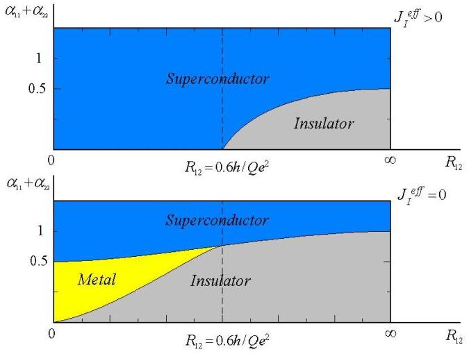
Figure 2: Phase diagram of the two band system for different values of $\alpha_{11}+\alpha_{22}$ versus $R_{12}$ for two values of $J_{I}$ with $J^{\rm eff}_{I}\neq 0$ in the upper panel and $J^{\rm eff}_{I}=0$ in the lower panel. A metallic phase is found in a narrow region of parameter space when $J^{\rm eff}_{I}=0$ and $R_{12}<0.6h/Qe^{2}$

To understand the phase diagram, we observe first that the phase diagram is divided into two regimes, (i)$J^{\rm eff}_{I}\neq 0$ (upper panel) and (ii)$J^{\rm eff}_{I}=0$ (lower panel). The effective Josephson coupling between the two bands is nonzero in the first regime and it is easy to show from Eqs. (7-9) that the two-band superconductor becomes effectively like a single band superconductor at low energy $\omega<<J^{\rm eff}_{I}$ in $S^{P}_{\rm trial}$. Correspondingly, $S^{n}_{\rm trial}$ becomes an effective one band model with $n_{i}^{1}\equiv n_{i}^{2}=n_{i}$ at temperature $T\rightarrow 0$ because of the $\beta J_{I}^{MS}\sum_{i}\delta(n_{i}^{1}-n_{i}^{2})$ term, i.e.

$$S^{n}_{\rm trial}\rightarrow{2\pi^{2}C_{t}\over\beta}\sum_{i}{\Delta_{\nu}n_{i}^{2}}+{Q\pi\over 4R_{\rm eff}}\sum_{i,\nu}|\Delta_{\nu}n_{i}|$$

when superconductivity is destroyed, where $C_{t}=C_{11}+C_{22}$ and $R_{\rm eff}^{-1}=R^{-1}_{11}+R^{-1}_{22}+2R^{-1}_{12}$. The system is at a roughening (insulator) phase when $R_{\rm eff}>R_{cI}=0.6(h/Qe^{2})$asos and a metallic phase exist only if $J_{aa}^{\rm eff}=0$ at a finite region of resistances $R_{cI}>R_{\rm eff}>R_{cS}$. For single-band superconductors, $R_{cS}=(h/Qe^{2})>R_{cI}$Ng (2001), and an intermediate metallic phase cannot exist in this case.

We next consider regime (ii) where $J^{\rm eff}_{I}=0$. First it is straightforward to show that $J^{\rm eff}_{I}\neq 0$ as long as $J^{\rm eff}_{aa}\neq 0$, indicating that the system behaves always like an effective one-band system at low enough energy in the superconducting state. The situation is different if superconductivity is destroyed. Substituting $J^{\rm eff}_{aa}=0$ into Eq. (8b), we obtain a self-consistent equation for $J^{\rm eff}_{I}$,

$$J^{\rm eff}_{I}=|J_{I}|P_{n}^{I}(0)\exp\left(-{1\over 2\beta Nd}\sum_{i\omega_{n},\vec{k}}{1\over J^{\rm eff}_{I}+\tilde{\alpha}_{I}|\omega_{n}|\gamma(\vec{k})}\right),$$ (10)

where $\tilde{\alpha}_{I}={\alpha_{11}\alpha_{22}+\alpha_{12}(\alpha_{11}+\alpha_{22})\over\alpha_{11}+\alpha_{22}+4\alpha_{12}}$.

Equation (10) is solved numerically where we find that the equation has a non-zero solution only when $|J_{I}|>J^{c}_{I}(\tilde{\alpha}_{I},J_{11})$, which is a number depending on $\tilde{\alpha}_{I}$ and roughly proportional to $\max(J_{11},J_{22})$, the transition from the $J^{\rm eff}_{I}\neq 0$ to $J^{\rm eff}_{I}=0$ state is a first order phase transition. The phase diagram determined by (10) is provided in the supplementary material.

This interesting result suggests that although the superconducting state behaves always like an effective one-band superconductor at low enough energy, there exists two kinds of non-superconducting states. The non-superconducting state is effectively one-band like when $J^{\rm eff}_{I}\neq 0$ and two-band like when $J^{\rm eff}_{I}=0$. We find that an intermediate metallic phase may exist in the two-band like non-superconducting state.

To see how this can occur we consider Eq. (8a) with $J^{\rm eff}_{I}=0$. In this case we obtain

$$J^{\rm eff}_{aa}\sim J_{aa}P_{n}^{aa}(0)\exp\left(-{1\over 2\beta Nd}\sum_{i\omega_{n},\vec{k}}{1\over J^{\rm eff}_{aa}+\tilde{\alpha}_{aa}|\omega_{n}|}\right),$$ (11)

where

$$\tilde{\alpha}_{aa}={h\over 4\pi e^{2}}\left({1\over R_{aa}}+{1\over R_{\bar{a}\bar{a}}+2R_{12}}\right),$$

corresponding to a single-band superconductor with effective resistance $R_{\rm eff}^{-1}=R_{aa}^{-1}+(R_{\bar{a}\bar{a}}+2R_{12})^{-1}$, which is the effective resistance obtained from the resistance network model shown in Fig.(1). The SI transition is determined by Eq. (11) and $S^{n}_{\rm trial}$. To see the plausible existence of metallic phase, we examine the limit $R_{12}^{\rm o}\sim R_{12}\rightarrow 0$. In this limit, a long-range order of $n^{1,2}_{i}$’s are built up in the winding number action $S^{n}_{\rm trial}$ because $n_{i}^{1}\equiv n_{i+\nu}^{2}\forall i$, and the system is always in the smooth phase. A metallic phase exists as long as $R_{\rm eff}\rightarrow R_{11}R_{22}/(R_{11}+R_{22})>h/Qe^{2}$ where $J^{\rm eff}_{aa}\rightarrow 0$.

The window for the existence of metallic phase narrowed down when $R_{12}$ increases as shown in Fig.(2) lower panel. Notice that the winding number field is basically controlled by $R_{12}$ when $R_{11}$ and $R_{22}$ are large, so for a metallic phase to occur, we generally require $R_{12}$ to be smaller than $0.6h/Qe^{2}$. For small $R_{12}$, the superconductor-insulator transition is governed by $\alpha_{11}+\alpha_{22}$. For the superconducting stiffness to vanish, we require $\alpha_{11}+\alpha_{22}\leq 0.5$.

The metallic phase, if exists, is a new state of matter with incoherent bosons participating in low temperature transports. The state is described by a Ginsburg-Landau (GL) theory with vanishing phase-stiffnessngepl . A preliminary analysis of the GL theory indicates that the system is a diamagnetic metal with unusual low-temperature magneto-transport behaviorsngepl .

To conclude, we re-examine the problem of SI transition in this paper for two-band superconductors, and raise again the question of plausible existence of metallic phase. Within a resistance-shunted Josephson network array model, we show that intermediate metallic phase between superconductor-insulator transition may exist for two-band superconducting films if the inter-band Josephson coupling $J_{I}$ and inter-band dissipative resistance term $R_{12}$ are small enough. Physically, the more complicated circuit network structure for two-band superconductors (Fig.1) gives rise to the possibility that the effective dissipation responsible for screening and quantum dissipation are coming from different resistance channels which is not possible for single-band superconductors. With the recent advancements of research in Iron pnictide and other multi-band superconductors, we believe that this new metallic phase of matter may be reachable in the near futureFW1101 .

This work is supported by HKRGC through grant HKUST3/CRF09.

I Supplementary materials

Here we show how the dissipative term  (2) can be derived from a straightforward generalization of the dissipative term for one-band system to two-band system. We assume phenomenologically that a metallic component exists in the system and the dissipative term can be derived from a Hamiltonian with tunnelling and capacitance energy between grains,

$$H=\sum_{m,a}H_{m}^{a}+\sum_{a,b}\left(H_{T}^{ab}+H_{Q}^{ab}\right)$$ (12)

where $m=L,R$ and $a,b=1,2$ are the grain and band indices, respectively.

$$H^{a}_{m}=\sum_{\sigma}\int dx_{m}\hat{\Psi}_{\sigma}^{\dagger a}(x_{m})[\epsilon^{a}_{m}(-i\nabla)]\hat{\Psi}_{\sigma}^{a}(x_{m})$$ (13a)

describes non-interacting electrons in grain $$m a \sigma$$, band where is the spin index, and

$$H_{T}^{ab}=\sum_{\sigma}\int dx_{L}dx_{R}T^{ab}(x_{L},x_{R})\hat{\Psi}_{\sigma}^{\dagger a}(x_{L})\hat{\Psi}_{\sigma}^{b}(x_{R})+h.c.$$ (13b)

describes tunneling of electrons between grain $$L a R b$$, band and grain , band and

$$H_{Q}^{ab}={1\over{8C}}(Q_{R}^{a}-Q_{L}^{b})^{2}$$ (13c)

is the charging energy associated with charge imbalance between the grains where

$$Q_{m}^{a}=e\sum_{\sigma}\int dx_{m}\hat{\Psi}_{\sigma}^{\dagger a}(x_{m})\hat{\Psi}_{\sigma}^{a}(x_{m})$$ (14)

is the total electric charge in grain $m$, band $a$. The corresponding action at imaginary time is

$$S =\sum_{a,\sigma}\int_{0}^{\beta}d\tau\{{\int dx_{L}{\bar{\Psi}_{\sigma}^{a}(x_{L})\partial\tau\Psi_{\sigma}^{a}(x_{L})}}$$ (15)

$$+\int dx_{R}{{\bar{\Psi}_{\sigma}^{a}(x_{R})\partial\tau\Psi_{\sigma}^{a}(x_{R})}}\}+H$$

To derive $S_{\rm diss}$ we first apply a Stratonovich-Hubbard transformation on $H_{Q}$ to obtain

$$S \rightarrow\sum_{m,a,\sigma}\int_{0}^{\beta}\int dx_{m}\bar{\Psi}_{\sigma}^{a}(x_{m})\{\partial\tau+\epsilon^{a}_{m}(-i\nabla)$$ (16)

$$+(-1)^{s_{m}}({{ie}\over{2}})[V_{aa}$$

$$+({{1+(-1)^{s_{m}}}\over{2}})V_{a\bar{a}}+({{1-(-1)^{s_{m}}}\over{2}})V_{\bar{a}a}]\}\Psi^{a}_{\sigma}(x_{m})$$

$$+\sum_{a,b,\sigma}\int_{0}^{\beta}d\tau\int dx_{L}dx_{R}$$

$$\times[T^{ab}(x_{L},x_{R})\bar{\Psi}^{a}_{\sigma}(x_{L})\Psi^{b}_{\sigma}(x_{R})+c.c]$$

$$-\sum_{a,b}\int_{0}^{\beta}d\tau[{{CV^{2}_{ab}}\over{2}}]$$

where $m=L,R$, $s_{L}=0$ and $s_{R}=1$ and $\bar{1}(\bar{2})=2(1)$.

Writing $V_{ab}=\dot{\theta}^{a}_{R}-\dot{\theta}^{b}_{L}$, where $\bar{L}(\bar{R})=R(L)$, the electric potential $V_{ab}$’s can be absorbed by a gauge transformation

$$\Psi^{a}_{\sigma}(x_{m},\tau)=e^{-i\theta_{m}^{a}+{{i}\over{2}}(\theta_{\bar{m}}^{1}+\theta_{\bar{m}}^{2})}\tilde{\Psi}^{a}_{\sigma}(x_{m},\tau).$$ (17)

where the tunnelling term becomes

$$S_{T} \rightarrow\sum_{a,b,\sigma}\int_{0}^{\beta}d\tau\int dx_{L}dx_{R}\{T^{ab}(x_{L},x_{R})$$ (18)

$$\times e^{i[{{1}\over{2}}(\Delta_{\nu}\theta^{ab}+\Delta_{\nu}\theta^{ba})+{{1}\over{2}}(\Delta_{\nu}\theta^{12}+\Delta_{\nu}\theta^{21})]}$$

$$\times\bar{\Psi}^{a}_{\sigma}(x_{L})\Psi^{b}_{\sigma}(x_{R})+c.c\}$$

where $\Delta_{\nu}\theta^{ab}=\theta_{L}^{a}-\theta_{R}^{b}$ $(a,b=1,2)$. To proceed further, we integrate out the fermionic fields and expand the tunnelling term to second order to obtain

$$S_{\rm eff}(\theta)=\sum_{a,b}\int_{0}^{\beta}d\tau[{C_{ab}\over 2}\Delta_{\nu}\dot{\theta}^{ab}(\tau)^{2}+S_{\rm diss}^{ab}]$$ (19)

where

$$S_{\rm diss}^{ab}={1\over 2}\sum_{\sigma}|T^{ab}|^{2}\int_{0}^{\beta}d\tau_{1}\int_{0}^{\beta}d\tau_{2}$$

$$\{G_{L\sigma}^{a}(\tau_{1}-\tau_{2})G_{R\sigma}^{b}(\tau_{2}-\tau_{1})e^{i(D_{\nu}\theta^{ab}(\tau_{2})-D_{\nu}\theta^{ab}(\tau_{1}))}$$

$$+G_{R\sigma}^{b}(\tau_{1}-\tau_{2})G_{L\sigma}^{a}(\tau_{2}-\tau_{1})e^{i(D_{\nu}\theta^{ba}(\tau_{1})-D_{\nu}\theta^{ba}(\tau_{2}))}\}$$

where $D_{\nu}\theta_{i}^{12}=D_{\nu}\theta_{i}^{21}=[\Delta_{\nu}\theta_{i}^{11}+\Delta_{\nu}\theta_{i}^{22}]$ and $D_{\nu}\theta_{i}^{aa}=[{{3}\over{2}}\Delta_{\nu}\theta_{i}^{aa}+{{1}\over{2}}\Delta_{\nu}\theta_{i}^{\bar{a}\bar{a}}]$.

$$G_{m\sigma}^{a}(\tau)={1\over{\beta V}}\sum_{i\omega,\vec{k}}{{e^{-i\omega_{n}\tau}}\over{i\omega_{n}-\epsilon_{m\sigma}^{a}(\vec{k})}}=-{D_{m\sigma}^{a}(E_{F})\pi T\over{\sin(\pi T\tau)}}$$ (21)

is the free electron Green’s function at imaginary time. $m=L,R$ and $D_{m\sigma}^{a}(E_{F})$ is the density of states on the Fermi surface. Defining

$$\alpha_{ab}^{o}(\tau) = \sum_{\sigma}|T^{ab}|^{2}D_{L\sigma}^{a}(E_{F})D_{R\sigma}^{b}(E_{F})({{\pi T}\over{\sin(\pi T\tau)}})^{2}$$ (22)

$$= \left({h\over 4e^{2}R_{ab}^{o}}\right)\left({T\over\sin(\pi T\tau)}\right)^{2}$$

and put it back into  (I) we obtain

$$S_{\rm diss} \sim\sum_{a,b}\int_{0}^{\beta}d\tau_{1}\int_{0}^{\beta}d\tau_{2}\{\alpha_{ab}^{o}(\tau_{1}-\tau_{2})$$

$$\times\sin^{2}[{{D_{\nu}\theta^{ab}(\tau_{1})-D_{\nu}\theta^{ab}(\tau_{2})}\over{2Q}}]\}$$

which is the dissipation term we use in the main text.

We attach here also the phase diagram determined by Eq. (10) with $J_{11}=J_{22}$. The line separating the $J_{I}^{\rm eff}=(\neq)0$ phases is a line of first order phase transition. we see that $J_{11}/J_{I}\sim\tilde{\alpha}_{I}={\alpha_{11}\alpha_{22}+\alpha_{12}(\alpha_{11}+\alpha_{22})\over\alpha_{11}+\alpha_{22}+4\alpha_{12}}$ at the transition.

Figure 3: Phase diagram for $J^{eff}_{I}$ for different values of $J_{I}^{-1}$ versus $\tilde{\alpha}$. A first order phase transition separates the $J_{I}^{eff}=0$ and $J_{I}^{eff}\neq 0$ phases

References

• M. P. A. Fisher (1982) M.Β P.Β A. Fisher, Phys. Rev. Lett. 65, 923 (1990).
• Chakravarty etΒ al. (1986) S.Β Chakravarty, G.Β  Ingold, S.Β  Kivelson, andΒ A.Β Luther, Phys. Rev. Lett. 56, 2303 (1986).
• Chakravarty etΒ al. (1987) S.Β Chakravarty, G.Β  Ingold, S.Β  Kivelson, andΒ G.Β Zimanyi, Phys. Rev. B 37, 3283 (1987).
• Kapitulnik etΒ al. (2001) A.Β Kapitulnik, N.Β  Mason, S.Β  Kivelson, andΒ S.Β Chakravarty, Phys. Rev. B. 63, 125322 (2001).
• (5) See for example, R. Fazio and G. Sch$\ddot{\text{o}}$n, Phys.Β Rev.Β B43, 5307 (1991) and J.E. Mooij et.al., Phys.Β Rev.Β Lett.Β 65, 645 (1990).
• (6) A.O. Caldeira and A.J. Leggett, Ann. Phys. (N.Y.) 149, 374 (1983).
• Ng (2001) Tai-Kai Ng, DerekΒ K.Β K. Lee, Phys. Rev. B 63, 144509 (2001).
• Suhl etΒ al. (1959) H.Β Suhl, B.Β T. Matthias, L.Β R.Walker, Phys. Rev. Lett. 3, 552 (1959).
• Nagamatsu etΒ al. (2001) Nagamatsu J.Β etΒ al., Nature 410, 63 (2001).
• (10) Y. Kamihara et al., J. Am. Chem. Soc. 130, 3296 (2008).
• (11) Ming-Hu Fang et al, Europhysics Lett. 94, 27009 (2011)
• (12) T.K. Ng, Europhysics Lett. 82, 47004 (2008)