On the initial shear field of the cosmic web

Abstract

The initial shear field, characterized by a primordial perturbation potential, plays a crucial role in the formation of large scale structures. Hence, considerable analytic work has been based on the joint distribution of its eigenvalues, associated with Gaussian statistics. In addition, directly related morphological quantities such as ellipticity or prolateness are essential tools in understanding the formation and structural properties of halos, voids, sheets and filaments, their relation with the local environment, and the geometrical and dynamical classification of the cosmic web. To date, most analytic work has been focused on Doroshkevich’s unconditional formulae for the eigenvalues of the linear tidal field, which neglect the fact that halos (voids) may correspond to maxima (minima) of the density field. I present here new formulae for the constrained eigenvalues of the initial shear field associated with Gaussian statistics, which include the fact that those eigenvalues are related to regions where the source of the displacement is positive (negative): this is achieved by requiring the Hessian matrix of the displacement field to be positive (negative) definite. The new conditional formulae naturally reduce to Doroshkevich’s unconditional relations, in the limit of no correlation between the potential and the density fields. As a direct application, I derive the individual conditional distributions of eigenvalues and point out the connection with previous literature. Finally, I outline other possible theoretically- or observationally-oriented uses, ranging from studies of halo and void triaxial formation, development of structure-finding algorithms for the morphology and topology of the cosmic web, till an accurate mapping of the gravitational potential environment of galaxies from current and future generation galaxy redshift surveys.

1 Introduction

The large-scale spatial distribution of dark matter, as revealed from numerical simulations, shows a characteristic anisotropic web-like structure. This cosmic web, which arises through the gravitational clustering of matter, is mainly due to the effects of the tidal field: in fact, the competition between cosmic expansion, the trace, and the traceless part of the tidal field imprints anisotropies in the large-scale matter distribution in much the same way that gravity and radiation pressure imprints baryonic acoustic oscillations (BAO) on the Cosmic Microwave Background (CMB) sky (Hu & Sugiyama 1995; Lee & Springel 2010). Hence, the initial shear field plays a crucial role in the formation of large scale structures, and a number of studies in the literature have been devoted to this subject – among the plethora of papers, see for example the classic works by Zeldovich (1970), Icke (1973), Peebles (1980), White (1984), Bardeen et al. (1986), Kaiser (1986), Bertschinger (1987), Bond & Myers (1996), Bond, Kofman & Pogosyan (1996) and van de Weygaert & Bertschinger (1996). In addition, if the cosmic web originates from primordial tidal effects and its degree of anisotropy increases with the evolution of the Universe, then studying this initial field is crucial in understanding the subsequent nonlinear evolution of cosmic structures (Springel et al. 2005; Shandarin et al. 2006; Desjacques 2008; Desjacques & Smith 2008; Pogosyan et al. 2009), the alignment of shape and angular momentum of halos (West 1989; Catelan et al. 2001; Lee & Springel 2010; Rossi, Sheth & Tormen 2011), the statistical properties of voids (Lee & Park 2006; Platen, van de Weygaert & Jones 2008), and more generally for characterizing the geometry and morphology of the cosmic web (Shen et al. 2006; van de Weygaert & Bond 2008; Forero-Romero et al. 2009; Aragon-Calvo et al. 2010a,b; Shandarin et al. 2010).

The basic theory for the formation and evolution of structures is now well-understood, thanks to the pioneering work of Doroshkevich & Zeldovich (1964), Doroshkevich (1970), Zeldovich (1970), and Sunyaev & Zeldovich (1972) – the latter in the context of galaxy formation. In particular, Doroshkevich (1970) derived the joint probability distribution of an ordered set of eigenvalues in the tidal field matrix – at random positions – given the variance of the density field, corresponding to a Gaussian potential; we will refer to it as the unconditional probability distribution of eigenvalues. In addition, Zeldovich (1970) provided the fundamental understanding of anisotropic collapse on cosmological scales, and recognized the key role of the large scale tidal force in shaping the cosmic web. Subsequently, Doroshkevich and Shandarin (1978) calculated some statistical properties of the maxima of the largest eigenvalue of the shear tensor. Their study proved that the most probable formation process starts first with a one-dimensional collapse (cosmic pancake formation). The directions (orientations) for the one-dimensional collapsed sheets are determined by the largest eigenvalue of the deformation tensor, which can be attributed to the initial linear density perturbations; moreover, the probability that two or even three of the initial eigenvalues are identical or nearly equal is extremely small, indicating that the collapse is triaxial. Later on, following a constrained field approach pioneered by Bertschinger (1987), van de Weygaert & Bertschinger (1996) developed an algorithm for setting up tailor-made initial conditions for cosmological simulations, which addressed the role of the tidal fields in shaping large-scale structures. In the same period, Bond, Kofman & Pogosyan (1996) developed a cosmic web theory which naturally explains the filamentary structure present in the Cold Dark Matter (CDM) cosmology, due to the coherent nature of the primordial tidal field. They realized that an “embryonic” cosmic web is already present in the primordial density field, and explained why in overdense regions sheet-like membranes are only marginal features. Since then, because of the correspondence between structures in the evolved density field and local properties of the linear tidal field pointed out by the same authors, the statistics of the shear has received more attention in the literature. For example, Lee & Shandarin (1998) computed some probability distributions for individual shear eigenvalues and obtained an analytic approximation to the halo mass function, and Catelan & Porciani (2001) explored the two-point correlation of the tidal shear components.

However, a variety of studies in the physics of halo formation and cosmic web classification are based on Doroshkevich’s unconditional formulae for the ordered eigenvalues of the initial shear field associated with Gaussian statistics (Doroshkevich 1970), but those formulas cannot differentiate between random positions and peak/dips as they neglect the fact that halos (voids) may correspond to maxima (minima) of the density field. According to Bardeen et al. (1986), if one assumes the cosmological density fluctuations to be Gaussian random fields, the local maxima of such fields are plausible sites for the formation of nonlinear structures. Hence, the statistical properties of the peaks can be used to predict the abundances and clustering properties of objects of various types, and in studies of the non-spherical formation of large-scale structures. The study of Bertschinger (1987) goes in this direction, by generalizing the treatment of Bardeen et al. (1986) and proposing a path integral method for sampling constrained Gaussian random fields. The method allows one to study the density field around peaks or other constrained regions in the biased galaxy formation scenario, but unfortunately it is too elaborate and inefficient in its implementation. Instead, by applying the prescription of Hoffman & Ribak (1991) to construct constrained random fields, van de Weygaert & Bertschinger (1996) were able to show that it is possible to generate efficiently initial Gaussian random density and velocity fields, and specify the presence and characteristics of one or more peaks and dips at arbitrary locations – with the gravity and tidal fields at the site of the peaks having the required strength and orientation. Some other studies on constrained initial conditions were also pursued by van Haarlem & van de Weygaert (1993), and by van de Weygaert & Babul (1994). The idea has been expanded in Bond & Myers (1996), who presented a peak-patch picture of structure formation as an accurate model of the dynamics of peaks in the density field. Their approach goes further, as it involves the explicit formalism for identifying objects in a multiscale field (i.e. it does not restrict to a single scale). The model is even more precise for void patches, the equivalent framework for studying voids (Sahni et al. 1994; Sheth & van de Weygaert 2004; Novikov, Colombi & Dore 2006; Colberg et al. 2008). In general, density peaks define a well-behaved point-process which can account for the discrete nature of dark matter halos and galaxies, and on asymptotically large scales are linearly biased tracers of the dark matter field (Desjacques & Sheth 2010).

Therefore, it would be desirable to incorporate the peak (or dip) constraint in the statistical description of the initial shear field, in order to characterize more realistically the geometry and dynamics of the cosmic web. The main goal of this paper is to do so, by providing a set of analytic expressions which extend the work of Doroshkevich (1970) and Bardeen et al. (1986), and are akin in philosophy to that of van de Weygaert & Bertschinger (1996). This is achieved by constraining the Hessian of the displacement field (the matrix of the second derivatives) to be positive (negative) definite, which is the case in the vicinity of minima (maxima) of the source of the displacement field. The new conditional probability distributions derived in this study include the correlation between the potential and density fields through a reduced parameter $r$, and naturally recover Doroshkevich’s (1970) unconditional formulae in the absence of correlation.

Hence, the main focus of this work is to derive explicitly the joint probability distribution of the eigenvalues of the shear field, given the fact that positions are peaks or dips in the corresponding density field – and not random locations. In this sense the field is termed constrained (i.e. it has constrained eigenvalues, which are the result of looking only at peak/dip regions), and it is statistically described by a conditional probability distribution. Note that even though the formalism is essentially restricted to one scale, the formulae derived here are useful in a variety of applications – some of which will be discussed at the end of this paper.

The layout is organized as follows. Section 2 provides the derivation of the new analytic expressions for the conditional distributions of eigenvalues of the initial shear field. In particular, Section 2.1 illustrates the basic notation adopted; Section 2.2 contains the derivation of the joint distribution of eigenvalues in the peak/dip picture, while Section 2.3 shows the reverse conditional distribution function. As a direct application of the new formulae, Section 3 presents the individual distributions of eigenvalues subjected to the extremum constraint, along with some other related conditional probabilities. This part extends previous work by Lee & Shandarin (1998), which is briefly summarized in Appendix A, and complements the study of van de Weygaert & Bertschinger (1996). Finally, Section 4 highlights the main results and discusses ongoing and future applications, which will be presented in forthcoming publications.

2 Joint distribution of eigenvalues at peak/dip locations

In this section, I first introduce the basic notation adopted throughout the paper. I then derive the conditional joint distribution of eigenvalues of the tidal field, under the constraint that the Hessian matrix of the source of the displacement is positive (or negative) definite. Finally, I present the reverse probability function, useful in relating this work with that of Bardeen et al. (1986) and van de Weygaert & Bertschinger (1996).

2.1 Basic notation

Let $\Psi$ denote the displacement field, $\Phi$ the potential of the displacement field, $S_{\rm\Psi}$ the source of the displacement field. Indicate with ${\bf q}$ the Lagrangian coordinate, with ${\bf x}$ the Eulerian coordinate, where

$${\bf x}({\bf q})={\bf q}+\Psi({\bf q}).$$ (1)

Use $T_{\rm ij}$ to denote the shear tensor of the displacement field, $H_{\rm ij}$ for the Hessian matrix, $J_{\rm ij}$ for the Jacobian of the displacement field ($i,j=1,2,3$). Clearly:

$$J_{\rm ij}({\bf q})={\partial x_{\rm i}\over\partial q_{\rm j}}=\delta_{\rm ij}+T_{\rm ij}$$ (2)

$$T_{\rm ij}={\partial\Psi_{\rm i}\over\partial q_{\rm j}}={\partial^{2}\Phi\over\partial q_{\rm i}\partial q_{\rm j}}$$ (3)

$$H_{\rm ij}={\partial^{2}S_{\Psi}\over\partial q_{\rm i}\partial q_{\rm j}}$$ (4)

$$S_{\Psi}({\bf q})=\sum_{\rm i=1}^{3}{\partial\Psi_{\rm i}\over\partial q_{\rm i}}\equiv\sum_{\rm i=1}^{3}{\partial^{2}\Phi\over\partial q^{2}_{\rm i}}.$$ (5)

The eigenvalues of $T_{\rm ij}$ are $\lambda_{1},\lambda_{2},\lambda_{3}$, those of $H_{\rm ij}$ are $\xi_{1},\xi_{2},\xi_{3}$. In general, the ordering of the eigenvalues is assumed to be such that $\lambda_{1}\geq\lambda_{2}\geq\lambda_{3}$. Let the potential $\Phi$ be a Gaussian random field determined by the power spectrum of matter density fluctuations $P(k)$, with $k$ denoting the wave number and $W(k)$ the smoothing kernel. The density field described by the source $S_{\Psi}$ is also a Gaussian random field. The correlations between these two fields are expressed by:

$$\langle T_{\rm ij}T_{\rm kl}\rangle={\sigma_{\rm T}^{2}\over 15}(\delta_{\rm ij}\delta_{\rm kl}+\delta_{\rm ik}\delta_{\rm jl}+\delta_{\rm il}\delta_{\rm jk})$$ (6)

$$\langle H_{\rm ij}H_{\rm kl}\rangle={\sigma_{\rm H}^{2}\over 15}(\delta_{\rm ij}\delta_{\rm kl}+\delta_{\rm ik}\delta_{\rm jl}+\delta_{\rm il}\delta_{\rm jk})$$ (7)

$$\langle T_{\rm ij}H_{\rm kl}\rangle={\Gamma_{\rm TH}^{2}\over 15}(\delta_{\rm ij}\delta_{\rm kl}+\delta_{\rm ik}\delta_{\rm jl}+\delta_{\rm il}\delta_{\rm jk})$$ (8)

where $\sigma_{\rm T}^{2}=S_{2}\equiv\sigma_{0}^{2}$, $\sigma_{\rm H}^{2}=S_{6}\equiv\sigma_{2}^{2}$, $\Gamma_{\rm TH}=-S_{4}\equiv-\sigma_{1}^{2}$, $\delta_{\rm ij}$ is the Kronecker delta, and

$$S_{\rm n}={1\over 2\pi^{2}}\int_{0}^{\infty}k^{\rm n}~{}P(k)~{}W^{2}(k){\rm d}k$$ (9)

$$\sigma_{\rm j}^{2}={1\over 2\pi^{2}}\int_{0}^{\infty}k^{\rm 2(j+1)}~{}P(k)~{}W^{2}(k)~{}{\rm d}k\equiv S_{\rm 2(j+1)}.$$ (10)

$T_{\rm ij}$ and $H_{\rm ij}$ are real symmetric tensors, so they are specified by 6 components (note however that only 5 are independent once the height of the density peak or dip has been set, because the trace of the shear field tensor is entirely constrained by the local density field value via the Poisson equation). Label them as $A=(1,1)$, $B=(2,2)$, $C=(3,3)$, $D=(1,2)$, $E=(1,3)$, $F=(2,3)$; the symbols $\alpha$ or $\beta$ indicate the various couples, in a compact notation, where $\alpha,\beta=A,B,C,D,E,F$. For example, if $\alpha=D$ then $T_{\alpha}=T_{\rm D}\equiv T_{12}$, and so forth. In the subsequent derivations, for clarity all the various dependencies on $\sigma$’s are dropped. This is done by introducing the “reduced” variables $\tilde{T}$ and $\tilde{H}$, defined as

$$\tilde{T}_{\alpha}=T_{\alpha}/\sigma_{\rm T},~{}~{}\tilde{\rm H}_{\alpha}=H_{\alpha}/\sigma_{\rm H}$$ (11)

and the “reduced” correlation

$$r=\Gamma_{\rm TH}/\sigma_{\rm T}\sigma_{\rm H}=-{\sigma_{1}^{2}\over\sigma_{0}\sigma_{2}}\equiv=-\gamma$$ (12)

where $\gamma$ is the same as in Eq. (4.6a) of Bardeen et al. (1986). In this notation, the eigenvalues of $\tilde{T}$ and of $\tilde{H}$ are $\tilde{\lambda}_{i}$’s and $\tilde{\xi}_{i}$’s, respectively, with $i=1,2,3$. Of course, the $\sigma$ dependence can be restored at any time, if desired, by using the previous Equations (11) and (12).

2.2 Joint conditional distribution of eigenvalues in the peak/dip picture

The main goal of this section is to derive the joint distribution of the eigenvalues of $J_{\rm ij}$ when the ordering is $\lambda_{1}\geq\lambda_{2}\geq\lambda_{3}$, in regions where the source of displacement $S_{\Psi}$ is a minimum (or maximum). Being a minimum (maximum) of $S_{\Psi}$ implies that the displacement field is such that the gradient of $S_{\Psi}$ is zero, and the Hessian matrix $\tilde{H}_{\alpha}$ is positive (or negative) definite. In block notation, the covariance matrix $\tilde{V}$ of the 12 reduced components of $Y=(\tilde{T},\tilde{H})$ is:

$$\tilde{V}=\begin{pmatrix}\langle\tilde{T}_{\alpha}\tilde{T}_{\alpha}\rangle&\langle\tilde{T}_{\alpha}\tilde{H}_{\beta}\rangle\\ \langle\tilde{H}_{\beta}\tilde{T}_{\alpha}\rangle&\langle\tilde{H}_{\beta}\tilde{H}_{\beta}\rangle\end{pmatrix}={1\over 15}\begin{pmatrix}A&rA\\ rA&A\end{pmatrix}$$ (13)

where

$$A=\begin{pmatrix}B&\oslash\\ \oslash&I\end{pmatrix},~{}B=\begin{pmatrix}3&1&1\\ 1&3&1\\ 1&1&3\end{pmatrix}$$ (14)

with $I$ a ($3\times 3$) identity matrix and $\oslash$ a ($3\times 3$) null matrix. The inverse of the reduced covariance matrix is simply:

$$\tilde{C}=\tilde{V}^{-1}={15\over(1-r^{2})}\begin{pmatrix}A^{-1}&-rA^{-1}\\ -rA^{-1}&A^{-1}\end{pmatrix}$$ (15)

where

$$A^{-1}=\begin{pmatrix}B^{-1}&\oslash\\ \oslash&I\end{pmatrix},~{}B^{-1}={1\over 10}\begin{pmatrix}4&-1&-1\\ -1&4&-1\\ -1&-1&4\end{pmatrix}.$$ (16)

The joint probability of observing a tidal field $\tilde{T}$ for the gravitational potential and a curvature $\tilde{H}$ for the density field (from now on, the understood indices $\alpha$ and $\beta$ are dropped) is a multivariate Gaussian in $Y=(\tilde{T},\tilde{H})$:

$$p(Y|r){\rm d}Y={e^{-{1\over 2}Y^{T}\cdot\tilde{C}\cdot Y}\over(2\pi)^{6}\sqrt{|\tilde{V}|}}{\rm d}Y\equiv p(\tilde{T},\tilde{H}|r){\rm d}\tilde{T}{\rm d}\tilde{H}.$$ (17)

Therefore

$$p(\tilde{T}|r,\tilde{H}>0)={\int_{\rm\tilde{H}>0}p(\tilde{T},\tilde{H}|r)~{}{\rm d}\tilde{H}\over p(\tilde{H}>0)}={\int_{\rm\tilde{H}>0}p(\tilde{H})\cdot p(\tilde{T}|r,\tilde{H})~{}{\rm d}\tilde{H}\over\int_{\rm\tilde{H}>0}p(\tilde{H})~{}{\rm d}\tilde{H}},$$ (18)

where

$$p(\tilde{T}|r,\tilde{H})={p(\tilde{T},\tilde{H}|r)\over p(\tilde{H})}={p(\tilde{T},\tilde{H}|r)\over\int_{\rm\tilde{T}}p(\tilde{T},\tilde{H}|r)~{}{\rm d}\tilde{T}}={e^{-{1\over 2}\rm(\tilde{T}-b)^{T}\cdot{\mathscr{A}}^{-1}\cdot(\tilde{T}-b)}\over(2\pi)^{3}\sqrt{|\mathscr{A}|}}.$$ (19)

The marginal distributions $p(\tilde{T})$ and $p(\tilde{H})$ are simply multidimensional Gaussians with covariance matrix $A/15$, and therefore they can be expressed using Doroshkevich’s formulae as

$$p(\tilde{T})={15^{3}\over 16\sqrt{5}\pi^{3}}e^{-\rm{3\over 2}(2k_{1}^{2}-5k_{2})}$$ (20)

with

$$k_{1} = \tilde{T}_{11}+\tilde{T}_{22}+\tilde{T}_{33}$$ (21)

$$k_{2} = \tilde{T}_{11}\tilde{T}_{22}+\tilde{T}_{11}\tilde{T}_{33}+\tilde{T}_{22}\tilde{T}_{33}-\tilde{T}^{2}_{12}-\tilde{T}^{2}_{13}-\tilde{T}^{2}_{23}$$ (22)

and similarly

$$p(\tilde{H})={15^{3}\over 16\sqrt{5}\pi^{3}}e^{-\rm{3\over 2}(2h_{1}^{2}-5h_{2})}$$ (23)

with

$$h_{1} = \tilde{H}_{11}+\tilde{H}_{22}+\tilde{H}_{33}$$ (24)

$$h_{2} = \tilde{H}_{11}\tilde{H}_{22}+\tilde{H}_{11}\tilde{H}_{33}+\tilde{H}_{22}\tilde{H}_{33}-\tilde{H}^{2}_{12}-\tilde{H}^{2}_{13}-\tilde{H}^{2}_{23}.$$ (25)

The conditional distribution $p(\tilde{T}|r,\tilde{H})$ is also a multidimensional Gaussian, with mean $b$ and covariance matrix $\mathscr{A}$, where

$$b=r\tilde{H},~{}{\mathscr{A}}={1\over 15}(1-r^{2})A.$$ (26)

Carrying on the calculation indicated in (19) yields:

$$p(\tilde{T}|r,\tilde{H})={15^{3}\over 16\sqrt{5}\pi^{3}}{1\over(1-r^{2})^{3}}{\rm exp}\Big{[}-{3\over 2(1-r^{2})}(2K_{1}^{2}-5K_{2})\Big{]}$$ (27)

where

$$K_{1} = (\tilde{T}_{11}-r\tilde{H}_{11})+(\tilde{T}_{22}-r\tilde{H}_{22})+(\tilde{T}_{33}-r\tilde{H}_{33})=k_{1}-rh_{1}$$

$$K_{2} = (\tilde{T}_{11}-r\tilde{H}_{11})(\tilde{T}_{22}-r\tilde{H}_{22})+(\tilde{T}_{11}-r\tilde{H}_{11})(\tilde{T}_{33}-r\tilde{H}_{33})$$ (28)

$$+ (\tilde{T}_{22}-r\tilde{H}_{22})(\tilde{T}_{33}-r\tilde{H}_{33})-(\tilde{T}_{12}-r\tilde{H}_{12})^{2}-(\tilde{T}_{13}-r\tilde{H}_{13})^{2}-(\tilde{T}_{23}-r\tilde{H}_{23})^{2}=k_{2}+r^{2}h_{2}-rh_{1}k_{1}+r\eta$$

and

$$\eta=\tilde{T}_{11}\tilde{H}_{11}+\tilde{T}_{22}\tilde{H}_{22}+\tilde{T}_{33}\tilde{H}_{33}+2\tilde{T}_{12}\tilde{H}_{12}+2\tilde{T}_{13}\tilde{H}_{13}+2\tilde{T}_{23}\tilde{H}_{23}$$ (29)

accounts for cross-correlation terms.

The previous expression (27) generalizes Doroshkevich’s formula (20) to include the fact that halos (voids) may correspond to maxima (minima) of the density field. Note that, if $r=0$, Doroshkevich’s formula (20) is indeed recovered – as expected in the limit of no correlations between the potential and density fields. Equation (27) is written in a Doroshkevich-like format, and it is one of the key results of this paper.

It is also possible to express (27) in terms of the constrained eigenvalues $\zeta^{\prime}$s of the ($\tilde{T}|r,\tilde{H}$) matrix. The result is:

$$p(\tilde{\zeta}_{1},\tilde{\zeta}_{2},\tilde{\zeta}_{3}|r) \equiv p(\tilde{\lambda}_{1},\tilde{\lambda}_{2},\tilde{\lambda}_{3}|r,\tilde{\xi}_{1},\tilde{\xi}_{2},\tilde{\xi}_{3})$$

$$= {15^{3}\over 8\sqrt{5}\pi}{1\over(1-r^{2})^{3}}{\rm exp}\Big{[}-{3\over 2(1-r^{2})}(2K_{1}^{2}-5K_{2})\Big{]}\cdot|(\tilde{\zeta}_{1}-\tilde{\zeta}_{2})(\tilde{\zeta}_{1}-\tilde{\zeta}_{3})(\tilde{\zeta}_{2}-\tilde{\zeta}_{3})|$$

where in terms of constrained eigenvalues:

$$K_{1} = \tilde{\zeta}_{1}+\tilde{\zeta}_{2}+\tilde{\zeta}_{3}=k_{1}-rh_{1}$$ (31)

$$K_{2} = \tilde{\zeta}_{1}\tilde{\zeta}_{2}+\tilde{\zeta}_{1}\tilde{\zeta}_{3}+\tilde{\zeta}_{2}\tilde{\zeta}_{3}=k_{2}+r^{2}h_{2}-rh_{1}k_{1}+r\eta$$ (32)

$$\eta = \tilde{\lambda}_{1}\tilde{\xi}_{1}+\tilde{\lambda}_{2}\tilde{\xi}_{2}+\tilde{\lambda}_{3}\tilde{\xi}_{3}$$ (33)

$$k_{1} = \tilde{\lambda}_{1}+\tilde{\lambda}_{2}+\tilde{\lambda}_{3}$$ (34)

$$k_{2} = \tilde{\lambda}_{1}\tilde{\lambda}_{2}+\tilde{\lambda}_{1}\tilde{\lambda}_{3}+\tilde{\lambda}_{2}\tilde{\lambda}_{3}$$ (35)

$$h_{1} = \tilde{\xi}_{1}+\tilde{\xi}_{2}+\tilde{\xi}_{3}$$ (36)

$$h_{2} = \tilde{\xi}_{1}\tilde{\xi}_{2}+\tilde{\xi}_{1}\tilde{\xi}_{3}+\tilde{\xi}_{2}\tilde{\xi}_{3}$$ (37)

with the partial distributions expressed by Doroshkevich’s unconditional formulae as

$$p(\tilde{\lambda}_{1},\tilde{\lambda}_{2},\tilde{\lambda}_{3})={15^{3}\over 8\sqrt{5}\pi}e^{\rm-{3\over 2}(2k_{1}^{2}-5k_{2})}(\tilde{\lambda}_{1}-\tilde{\lambda}_{2})(\tilde{\lambda}_{1}-\tilde{\lambda}_{3})(\tilde{\lambda}_{2}-\tilde{\lambda}_{3}),$$ (38)

$$p(\tilde{\xi}_{1},\tilde{\xi}_{2},\tilde{\xi}_{3})={15^{3}\over 8\sqrt{5}\pi}e^{\rm-{3\over 2}(2h_{1}^{2}-5h_{2})}(\tilde{\xi}_{1}-\tilde{\xi}_{2})(\tilde{\xi}_{1}-\tilde{\xi}_{3})(\tilde{\xi}_{2}-\tilde{\xi}_{3}).$$ (39)

and

$$\tilde{\zeta}_{\rm i}\equiv(\tilde{\lambda}_{\rm i}|r,\tilde{\xi}_{\rm i})=\tilde{\lambda}_{\rm i}-r\tilde{\xi}_{\rm i}$$ (40)

which is obvious from (2.2), with $\tilde{\lambda}_{\rm i}$’s and $\tilde{\xi}_{\rm i}$’s the corresponding unconstrained eigenvalues of the matrices $\tilde{T}$ and $\tilde{H}$. Equation (2.2) is another key result of this work. This relation is easily derived from (27) because the volume element in the six-dimensional space of symmetric real matrices is simply given, in terms of constrained eigenvalues, by

$$\prod_{\alpha}{\rm d}(\tilde{T}_{\alpha}|r,\tilde{H}_{\alpha})=|(\tilde{\zeta}_{1}-\tilde{\zeta}_{2})(\tilde{\zeta}_{2}-\tilde{\zeta}_{3})(\tilde{\zeta}_{1}-\tilde{\zeta}_{3})|{\rm d}\tilde{\zeta}_{1}{\rm d}\tilde{\zeta}_{2}{\rm d}\tilde{\zeta}_{3}{\rm d}\Omega_{\rm S^{3}}$$ (41)

where ${\rm d}\Omega_{S^{3}}$ is the volume element of the three-dimensional rotation group $SO(3)$, and also of the three-sphere (see Appendix B in Bardeen et al. 1986). In addition, from (2.2) it is direct to see that one has $\tilde{T}_{\rm ii}\equiv\tilde{\lambda}_{\rm i}$ and $\tilde{H}_{\rm ii}\equiv\tilde{\xi}_{\rm i}$ in the system where both $\tilde{T}$ and $\tilde{H}$ are diagonal; therefore $K_{1}=\sum_{\rm i}(\tilde{\lambda}_{\rm i}-r\tilde{\xi}_{\rm i})\equiv\sum_{\rm i}\zeta_{\rm i}$, with $\zeta_{\rm i}$ the constrained eigenvalues.

The fact that the system in which $\tilde{T}$ is diagonal is also the system in which $\tilde{H}$ is diagonal has a simple geometrical explanation: in order to obtain the conditional distribution ($\tilde{T}|r,\tilde{H}$), a standard procedure for multivariate Gaussians (when transforming from uncorrelated to correlated variates) is to use a Cholesky decomposition. However, this decomposition does not sample symmetrically with respect to the principal axes. An alternative method which takes care of the alignment with the principal axes (and used here) is the following: decompose spectrally the covariance matrix of ($\tilde{T}|r,\tilde{H}$), ${\cal A}$, i.e. find the eigensystem $D$ and diagonal eigenvalue matrix $\Lambda$ of the covariance matrix such that ${\cal A}=D\cdot\Lambda\cdot D^{\rm T}$; then set $W=D\cdot\Lambda^{1/2}Y$, with $Y$ a set of independent zero mean unit variance Gaussians. It is direct to show that $W$ is indeed the correct covariance matrix, and this scheme takes care of the alignment with the principal axes.

2.3 The reverse joint conditional distribution of eigenvalues

Equation (18) expresses the probability of observing a tidal field $\tilde{T}$ in regions where the curvature $\tilde{H}$ of the density field is positive/negative (i.e. peak or dip regions). One may be also interested in the reverse joint conditional distribution, namely $p(\tilde{H}|r,\tilde{T}>0)$. Obtaining its expression is easily achieved from the previous algebra by applying Bayes’ theorem, so that:

$$p(\tilde{H}|r,\tilde{T}>0)={\int_{\tilde{T}>0}p(\tilde{H},\tilde{T}|r)~{}{\rm d}\tilde{T}\over p(\tilde{T}>0)}={\int_{\tilde{T}>0}p(\tilde{T})~{}{\rm d}\tilde{T}\cdot p(\tilde{H}|r,\tilde{T})\over\int_{\tilde{T}>0}p(\tilde{T})~{}{\rm d}\tilde{T}}$$ (42)

where now (symmetrically)

$$p(\tilde{H}|r,\tilde{T})={p(\tilde{H},\tilde{T}|r)\over p(\tilde{T})}={p(\tilde{H},\tilde{T}|r)\over\int_{\rm\tilde{H}}p(\tilde{H},\tilde{T}|r)~{}{\rm d}\tilde{H}}={e^{-\rm{1\over 2}(\tilde{H}-b^{\prime})^{\rm T}\cdot{\mathscr{A}}^{-1}\cdot(\tilde{H}-b^{\prime})}\over(2\pi)^{3}\sqrt{|\mathscr{A}|}}.$$ (43)

The distribution $p(\tilde{H}|r,\tilde{T})$ is also a multidimensional Gaussian with mean $b^{\prime}$ and covariance matrix $\mathscr{A}$, where

$$b^{\prime}=r\tilde{T},~{}{\mathscr{A}}={1\over 15}(1-r^{2})A.$$ (44)

Along the lines of the previous calculation, it is direct to obtain

$$p(\tilde{H}|r,\tilde{T})={15^{3}\over 16\sqrt{5}\pi^{3}}{1\over(1-r^{2})^{3}}{\rm exp}\Big{[}-{3\over 2(1-r^{2})}(2H_{1}^{2}-5H_{2})\Big{]}$$ (45)

where in analogy with (27) one has now:

$$H_{1} = (\tilde{H}_{11}-r\tilde{T}_{11})+(\tilde{H}_{22}-r\tilde{T}_{22})+(\tilde{H}_{33}-r\tilde{T}_{33})=h_{1}-rk_{1}$$

$$H_{2} = (\tilde{H}_{11}-r\tilde{T}_{11})(\tilde{H}_{22}-r\tilde{T}_{22})+(\tilde{H}_{11}-r\tilde{T}_{11})(\tilde{H}_{33}-r\tilde{T}_{33})$$ (46)

$$+ (\tilde{H}_{22}-r\tilde{T}_{22})(\tilde{H}_{33}-r\tilde{T}_{33})-(\tilde{H}_{12}-r\tilde{T}_{12})^{2}-(\tilde{H}_{13}-r\tilde{T}_{13})^{2}-(\tilde{H}_{23}-r\tilde{T}_{23})^{2}=h_{2}+r^{2}k_{2}-rk_{1}h_{1}+r\eta.$$

In addition, if $\epsilon_{1},\epsilon_{2},\epsilon_{3}$ are the constrained eigenvalues of ($\tilde{H}|r,\tilde{T}$), then

$$p(\tilde{\epsilon}_{1},\tilde{\epsilon}_{2},\tilde{\epsilon}_{3}|r) \equiv p(\tilde{\xi}_{1},\tilde{\xi}_{2},\tilde{\xi}_{3}|r,\tilde{\lambda}_{1},\tilde{\lambda}_{2},\tilde{\lambda}_{3})$$

$$= {15^{3}\over 8\sqrt{5}\pi}{1\over(1-r^{2})^{3}}{\rm exp}\Big{[}-{3\over 2(1-r^{2})}(2H_{1}^{2}-5H_{2})\Big{]}\cdot|(\tilde{\epsilon}_{1}-\tilde{\epsilon}_{2})(\tilde{\epsilon}_{1}-\tilde{\epsilon}_{3})(\tilde{\epsilon}_{2}-\tilde{\epsilon}_{3})|$$

where in terms of constrained eigenvalues

$$H_{1} = \tilde{\epsilon}_{1}+\tilde{\epsilon}_{2}+\tilde{\epsilon}_{3}=h_{1}-rk_{1}$$ (48)

$$H_{2} = \tilde{\epsilon}_{1}\tilde{\epsilon}_{2}+\tilde{\epsilon}_{1}\tilde{\epsilon}_{3}+\tilde{\epsilon}_{2}\tilde{\epsilon}_{3}=h_{2}+r^{2}k_{2}-rh_{1}k_{1}+r\eta,$$ (49)

with the $\epsilon_{\rm i}$’s simply given by

$$\tilde{\epsilon}_{\rm i}\equiv(\tilde{\xi}_{\rm i}|r,\tilde{\lambda}_{\rm i})=\tilde{\xi}_{\rm i}-r\tilde{\lambda}_{\rm i}.$$ (50)

Note an interesting symmetry: $K_{1}$, $H_{1}$, $k_{1}$, $h_{1}$ are always the traces of their corresponding matrices.

New analytic formulae derived from (45) and (2.3), which generalize the work of Bardeen et al. (1986), will be presented in a forthcoming publication. The previous relations are also useful in making the connection with the work of van de Weygaert & Bertschinger (1996). For example, Equation (50) confirms their finding of the correlation between the shifted mean values for density and shear (see for example Equation 108 in van de Weygaert & Bertschinger 1996, which provides the reverse mean value of the shear given a density field shape, and their Section 4.4 for more details).

3 Individual conditional distributions and probabilities

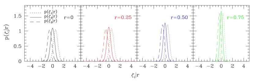
Figure 1: Individual conditional distributions $p(\zeta_{\rm i}|r)$ of the initial shear field in the peak/dip picture (Equations 3, 3 and 3), for different values of the reduced correlation parameter $r$ – as indicated in the panels.

A direct application of the main formulae derived in Section 2.2 is to compute the individual distributions of eigenvalues (along with some other related conditional probabilities), given the peak/dip constraint. Starting from Equation (2.2), with some extra complications due to the inclusion of correlation terms, it is possible to extend the work of Lee & Shandarin (1998) to account for those regions where the source of the displacement is positive (negative) – see the Appendix A for a compact summary of their results. Introducing the following notation:

$$l = {1125\over 64\sqrt{5}\pi}$$ (51)

$$l^{\prime} = l\cdot(1-r^{2})^{-5/2}$$

$$n = \sqrt{3\pi}/12$$

$$L^{\prime}(x,y|r) = \sqrt{1-r^{2}}~{}(x-y)(3x-y)\cdot{\rm exp}\Big{[}-{3\over(1-r^{2})}\Big{(}x^{2}-xy+{3\over 2}y^{2}\Big{)}\Big{]}$$

$$N^{\prime}(x,y|r) = (x-y)[8(1-r^{2})+3(3x-y)(3y-x)]\cdot{\rm exp}\Big{[}-{15\over 16(1-r^{2})}\Big{(}3x^{2}-2xy+3y^{2}\Big{)}\Big{]}\cdot{\rm erfc}\Big{[}{\sqrt{3}\over 4}{1\over\sqrt{1-r^{2}}}(x-3y)\Big{]}$$

and dropping the understood $\sim$ symbol (but note that the eigenvalues are still “reduced variables”), the two-point probability distributions of the constrained eigenvalues of the shear field are given by:

$$p(\zeta_{1},\zeta_{2}|r) = l^{\prime}\Big{[}L^{\prime}(\zeta_{1},\zeta_{2}|r)+n\cdot N^{\prime}(\zeta_{1},\zeta_{2}|r)\Big{]}$$ (52)

$$p(\zeta_{2},\zeta_{3}|r) = l^{\prime}\Big{[}L^{\prime}(\zeta_{3},\zeta_{2}|r)+n\cdot N^{\prime}(\zeta_{3},\zeta_{2}|r)\Big{]}$$

$$p(\zeta_{1},\zeta_{3}|r) = l^{\prime}\Big{\{}L^{\prime}(\zeta_{1},\zeta_{3}|r)+L^{\prime}(\zeta_{3},\zeta_{1}|r)+n\cdot\Big{[}N^{\prime}(\zeta_{1},\zeta_{3}|r)+N^{\prime}(\zeta_{3},\zeta_{1}|r)\Big{]}\Big{\}}.$$

Performing the various partial integrations, it is straightforward to obtain:

$$p(\zeta_{1}|r) = l^{\prime}\Big{\{}\int_{-\infty}^{\zeta_{1}}L^{\prime}(\zeta_{1},\zeta_{2}|r){\rm d}\zeta_{2}+n\int_{-\infty}^{\zeta_{1}}N^{\prime}(\zeta_{1},\zeta_{2}|r){\rm d}\zeta_{2}\Big{\}}$$

$$= {\sqrt{5}\over 12\pi}\Big{[}{20\over(1-r^{2})}\zeta_{1}~{}{\rm exp}\Big{(}-{9\zeta_{1}^{2}\over 2(1-r^{2})}\Big{)}-{\sqrt{2\pi}\over(1-r^{2})^{3/2}}~{}{\rm exp}\Big{(}-{5\zeta_{1}^{2}\over 2(1-r^{2})}\Big{)}\cdot{\rm erfc}\Big{(}-{\sqrt{2}\zeta_{1}\over\sqrt{1-r^{2}}}\Big{)}[(1-r^{2})-20\zeta_{1}^{2}]$$

$$+{3\sqrt{3\pi}\over\sqrt{1-r^{2}}}~{}{\rm exp}\Big{(}-{15\zeta_{1}^{2}\over 4(1-r^{2})}\Big{)}{\rm erfc}\Big{(}-{\sqrt{3}\zeta_{1}\over 2\sqrt{1-r^{2}}}\Big{)}\Big{]}$$

$$p(\zeta_{2}|r) = l^{\prime}\Big{\{}\int_{\zeta_{2}}^{+\infty}L^{\prime}(\zeta_{1},\zeta_{2}|r){\rm d}\zeta_{1}+n\int_{\zeta_{2}}^{+\infty}N^{\prime}(\zeta_{1},\zeta_{2}|r){\rm d}\zeta_{1}\Big{\}}$$

$$= {\sqrt{15}\over 2\sqrt{\pi}}{1\over\sqrt{1-r^{2}}}{\rm exp}\Big{[}-{15\over 4}{\zeta_{2}^{2}\over(1-r^{2})}\Big{]}$$

$$p(\zeta_{3}|r) = l^{\prime}\Big{\{}\int_{\zeta_{3}}^{\zeta_{1}}L^{\prime}(\zeta_{3},\zeta_{2}|r){\rm d}\zeta_{2}+n\int_{\zeta_{3}}^{\zeta_{1}}N^{\prime}(\zeta_{3},\zeta_{2}|r){\rm d}\zeta_{2}\Big{\}}$$

$$= -{\sqrt{5}\over 12\pi}\Big{[}{20\over(1-r^{2})}\zeta_{3}~{}{\rm exp}\Big{(}-{9\zeta_{3}^{2}\over 2(1-r^{2})}\Big{)}+{\sqrt{2\pi}\over(1-r^{2})^{3/2}}~{}{\rm exp}\Big{(}-{5\zeta_{3}^{2}\over 2(1-r^{2})}\Big{)}\cdot{\rm erfc}\Big{(}{\sqrt{2}\zeta_{3}\over\sqrt{1-r^{2}}}\Big{)}[(1-r^{2})-20\zeta_{3}^{2}]$$

$$-{3\sqrt{3\pi}\over\sqrt{1-r^{2}}}~{}{\rm exp}\Big{(}-{15\zeta_{3}^{2}\over 4(1-r^{2})}\Big{)}{\rm erfc}\Big{(}{\sqrt{3}\zeta_{3}\over 2\sqrt{1-r^{2}}}\Big{)}\Big{]}.$$

Plots of these distributions are shown in Figure 1, for different values of the reduced correlation $r$. Note the symmetry between $p(\zeta_{1}|r)$ and $p(\zeta_{3}|r)$, evident from (3) and (3). In particular, $p(\zeta_{2}|r)$ is simply a Gaussian with variance $2(1-r^{2})/15$, and so the conditional distribution $p(\lambda_{2}|r,\xi_{2})$ is a Gaussian with the same variance and shifted mean $r\xi_{2}$ (recall that $\zeta_{2}=\lambda_{2}-r\xi_{2}$). In addition, it is easy to show that, with $\Delta=\zeta_{1}+\zeta_{2}+\zeta_{3}\equiv K_{1}$, one obtains

$$p(\Delta,\zeta_{3}|r) = {3\sqrt{5}\over 16\pi}{1\over(1-r^{2})^{2}}\Big{[}15\Delta^{2}-90\Delta\zeta_{3}+135\zeta_{3}^{2}-8(1-r^{2})\Big{]}\cdot{\rm exp}\Big{[}-{3\over 8(1-r^{2})}(3\Delta^{2}-10\Delta\zeta_{3}+15\zeta_{3}^{2})\Big{]}$$ (56)

$$+{3\sqrt{5}\over 2\pi}{1\over(1-r^{2})}{\rm exp}\Big{[}-{3\over(1-r^{2})}\Big{(}\Delta^{2}-5\Delta\zeta_{3}+{15\over 2}\zeta_{3}^{2}\Big{)}\Big{]}.$$

By integrating the previous equation over $\zeta_{3}$, it is direct to verify that $p(\Delta|r)\equiv p(K_{1}|r)$ is a Gaussian with zero mean and variance $(1-r^{2})$, namely:

$$p(\Delta|r)={1\over\sqrt{2\pi(1-r^{2})}}\cdot{\rm exp}\Big{[}-{\Delta^{2}\over 2(1-r^{2})}\Big{]}\equiv p(K_{1}|r).$$ (57)

Since $K_{1}=k_{1}-rh_{1}$ (i.e. Eq. 31), the previous expression implies that $p(k_{1}|r,h_{1})$ is therefore a Gaussian with mean $rh_{1}$ and variance $(1-r^{2})$. In addition:

$$p(\zeta_{1}>0|r) = {23\over 25},~{}~{}~{}\langle\zeta_{1}|r\rangle={3\over\sqrt{10\pi}}\sqrt{1-r^{2}},~{}~{}~{}~{}\sigma^{2}_{\rm\zeta_{1}|r}={13\pi-27\over 30\pi}(1-r^{2})$$ (58)

$$p(\zeta_{2}>0|r) = {1\over 2},~{}~{}~{}~{}~{}\langle\zeta_{2}|r\rangle=0,~{}~{}~{}~{}~{}~{}~{}~{}~{}~{}\sigma^{2}_{\rm\zeta_{2}|r}={2\over 15}(1-r^{2})$$ (59)

$$p(\zeta_{3}>0|r) = {2\over 25},~{}~{}~{}\langle\zeta_{3}|r\rangle=-{3\over\sqrt{10\pi}}\sqrt{1-r^{2}},~{}~{}\sigma^{2}_{\rm\zeta_{3}|r}={13\pi-27\over 30\pi}(1-r^{2}).$$ (60)

Moreover, the probability distribution of $\Delta$ confined in the regions with $\zeta_{3}>0$ is:

$$p(\Delta|r,\zeta_{3}>0) = {p(\Delta,\zeta_{3}>0|r)\over p(\zeta_{3}>0)}={\int_{0}^{\rm\Delta/3}p(\Delta,\zeta_{3}|r){\rm d}\zeta_{3}\over p(\zeta_{3}>0)}$$

$$= -{75\sqrt{5}\over 8\pi}{\Delta\over(1-r^{2})}~{}{\rm exp}\Big{(}-{9\over 8}{\Delta^{2}\over(1-r^{2})}\Big{)}+$$

$$+ {25\over 4\sqrt{2\pi}}{1\over\sqrt{1-r^{2}}}~{}{\rm exp}\Big{(}-{\Delta^{2}\over 2(1-r^{2})}\Big{)}\Big{[}{\rm erf}\Big{(}{\sqrt{10}\Delta\over 4\sqrt{1-r^{2}}}\Big{)}+{\rm erf}\Big{(}{\sqrt{10}\Delta\over 2\sqrt{1-r^{2}}}\Big{)}\Big{]}.$$

Using the previous formula, it is direct to prove that

$$\langle\Delta|r,\zeta_{3}>0\rangle={25\sqrt{10}\over 144\sqrt{\pi}}(3\sqrt{6}-2)~{}\sqrt{1-r^{2}}\simeq 1.6566~{}\sqrt{1-r^{2}}.$$ (62)

Figure 2 shows the conditional probability distribution $p(K_{1}|r,\zeta_{3}>0)\equiv p(\Delta|r,\zeta_{3}>0)$ (i.e. Equation 3), for different values of $r$. The dotted vertical lines display the average values of those functions, as given in (62), while the vertical solid lines indicate their maximum values. In fact, it is easy to see that the maximum of $p(\Delta|r,\zeta_{3}>0)$ is reached when $\Delta\simeq 1.5~{}\sqrt{1-r^{2}}$. This result is readily obtained by computing the derivative of $p(\Delta|r,\zeta_{3}>0)$, and by finding the corresponding zeroes. An example of this calculation is shown in Figure 3, where an arbitrary value of $r=0.5$ is considered.

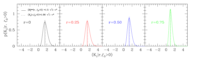
Figure 2: Conditional probability distribution $p(K_{1}|r,\zeta_{3}>0)\equiv p(\Delta|r,\zeta_{3}>0)$ given by Equation (3), for different values of $r$, as indicated in the panels. Solid vertical lines show the maximum of each distribution ($K_{1}^{\rm max}\simeq 1.5~{}\sqrt{1-r^{2}}$), dotted lines represent their corresponding average values as given by Equation (62).

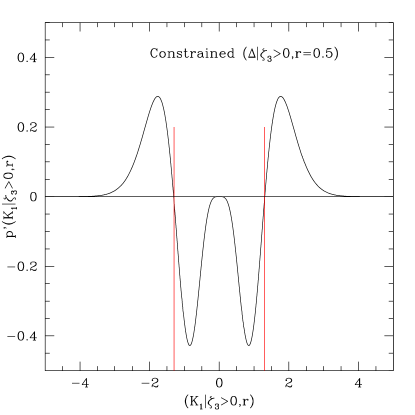
Figure 3: Determination of the maxima of (3). The derivative $p^{\prime}(K_{1}|\zeta_{3}>0,r)$ is shown, for an arbitrary value of the reduced correlation $r$, i.e. $r=0.5$. The maxima correspond to those points where $K_{1}^{\rm max}\simeq 1.5~{}\sqrt{1-r^{2}}$, indicated with solid vertical lines in the figure.

Finally, the probability that a given region with density $\Delta$ will have all positive eigenvalues $\zeta$’s is:

$$p(\zeta_{3}>0|\Delta,r)={p(\Delta,\zeta_{3}>0|r)\over p(\Delta|r)}=-{3\sqrt{10}\over 4\sqrt{\pi}}{\Delta\over\sqrt{1-r^{2}}}~{}{\rm exp}\Big{(}-{5\over 8}{\Delta^{2}\over(1-r^{2})}\Big{)}+{1\over 2}\Big{[}{\rm erf}\Big{(}{\sqrt{10}\Delta\over 4\sqrt{1-r^{2}}}\Big{)}+{\rm erf}\Big{(}{\sqrt{10}\Delta\over 2\sqrt{1-r^{2}}}\Big{)}\Big{]}.$$

Note that, in absence of correlations between the potential and density fields (i.e. when $r=0$), all the previous expressions reduce consistently to the unconditional limit of Lee & Shandarin (1998) – see again Appendix A. Several other results on probability distributions along these lines were also already derived by van de Weygaert & Bertschinger (1996): here we confirm their findings that the inclusion of the condition for a peak or dip in the Gaussian density field involves a $1/\sqrt{1-r^{2}}$ factor, and that the conditional distributions have shifted mean and reduced variance (see again their Section 4).

4 CONCLUSION

Since the initial shear field associated with Gaussian statistics plays a major role in the formation of large scale structures, considerable analytic work has been based on the joint distribution of its eigenvalues – i.e. Doroshkevich’s formulae (Equation 20). However, Doroshkevich’s equations neglect the fact that halos (voids) may correspond to maxima (minima) of the density field. The main goal of this work was to provide new analytic expressions, in the context of the peak/dip picture (Bardeen et al. 1986; Bond et al. 1991), which include the fact that the eigenvalues of the linear shear field are related to regions where the source of the displacement is positive (negative). These new conditional probabilities, derived in Section 2, are Equations (27), (2.2), (45) and (2.3): they represent the main results of this paper. Written in Doroshkevich-like format, they naturally reduce to Doroshkevich’s (1970) unconditional relations in the limit of no correlation between the potential and the density fields (i.e. when $r=0$). As a first direct application of (2.2), the individual conditional distributions of eigenvalues were obtained in Section 3; these relations extend some previous work by Lee & Shandarin (1998) – see Appendix A for a compact summary of their results. Much more analytic work can be carried out using these new formulae, especially in connection with the statistics of peaks developed by Bardeen et al. (1986): their calculations can be extended within this framework (see Section 2.3), and results of this extension will be presented in a forthcoming publication – along with more insights on the equations derived in Section 2.2.

To obtain the conditional distribution $p(\tilde{T}|r,\tilde{H}>0)$ (i.e. Equation 18), in principle one needs to sample numerically the probability (19) as done in Lavaux & Wandelt (2010). However, the new analytic results of this paper suggest a simpler generalized excursion set algorithm, which will be also presented in a forthcoming study. The algorithm allows for a fast sampling of (19), and permits to test the new relations derived here (i.e. Sections 2 and 3, and Appendix A) against mock data. In addition, along these lines it is possible to extend the main shape distributions involved in the triaxial formation of nonlinear structures (i.e. ellipticity $e$, prolateness $p$, axis ratios $\nu$ and $\mu$, etc.). Halos and voids are in fact triaxial rather than spherical (i.e. Rossi, Sheth & Tormen 2011), and the initial shear field plays a crucial role in their formation. For example, in the ellipsoidal collapse framework the virialization condition depends on ellipticity and prolateness, which are directly related to the eigenvalues of the external tidal field. Starting from $p(\zeta_{1},\zeta_{2},\zeta_{3}|r)$, it is then straightforward to turn this joint conditional distribution into $p(e,p,\delta|r)$ – to include the peak constrain, – and then to characterize $p(e|r)$, $p(p|r)$, $p(\mu|r)$, $p(\nu|r)$ and so forth. Applications to halos and voids will be also presented next, including implications for the skeleton of the cosmic web. The extension to non-Gaussian fields, along the lines of Lam et al. (2009), is a natural follow-up of this work and will be presented in a forthcoming publication as well. In the context of cosmic voids, other interesting uses of the new formulae (27), (2.2), (45) and (2.3) involve the Monge-Ampère-Kantorovitch reconstruction procedure – see for example Lavaux & Wandelt (2010).

The analytic framework described here can be also useful in several observationally-oriented applications, and in particular for developing algorithms to find and classify structures in the cosmic web. For example, Bond, Strauss & Cen (2010) presented an algorithm that uses the eigenvectors of the Hessian matrix of the smoothed galaxy distribution to identify individual filamentary structures. They used the distribution of the Hessian eigenvalues of the smoothed density field on a grid to study clumps, filaments and walls. Other possibilities include a web classification based on the multiscale analysis of the Hessian matrix of the density field (Aragon-Calvo et al. 2007), the skeleton analysis (Novikov et al. 2006), as well as a morphological (Zeldovich-based) classification (for instance Klypin & Shandarin 1983; Forero-Romero et al. 2009). More generally, the fact that the eigenvalues of the Hessian matrix can be used to discriminate different types of structure in a particle distribution is fundamental to a number of structure-finding algorithms (Forero-Romero et al. 2009), shape-finders algorithms (Sahni et al. 1998), and structure reconstruction on the basis of tessellations (Schaap & van de Weygaert 2000; Romano-Diaz & van de Weygaert 2007), etc. In addition, the classification of different environments should provide a framework for studying the environmental dependence of galaxy formation (see for example Blanton et al. 2005). To this end, recently Park, Kim and Park (2010) extended the concept of galaxy environment to the gravitational potential and its functions – as the shear tensor. They studied how to accurately estimate the gravitational potential from an observational sample finite in volume, biased due to galaxy biasing, and subject to redshift space distortions, by inspecting the dependence of dark matter halo properties on environmental parameters (i.e. local density, gravitational potential, ellipticity and prolateness of the shear tensor). It would be interesting to interpret their results with the theoretical formalism developed here, and ultimately to study the gravitational potential directly from a real dataset such as the SDSS Main Galaxy sample within this framework.

The formalism presented in this paper is restricted to one scale (i.e. peaks and dips in the density field, as in Bardeen et al. 1986), but the extension to a multiscale peak-patch approach along the lines of Bond & Myers (1996) is duable and subject of ongoing work. This will allow to account for the role of the peculiar gravity field itself, an important aspect not considered here but discussed for example in van de Weygaert & Bertschinger (1996). In fact, these authors introduced the peak constraints to describe the density field in the immediate surroundings of a peak, and then addressed the constraints on the gravitational potential perturbations; in particular, they constrained the peculiar gravitational acceleration at the position of the peak itself, in addition to characterizing the tidal field around the peak. Including all these effects in our formalism is ongoing effort. Finally, the interesting and more complex question of the local expected density field alignment/orientation distribution as a function of the local field value (or the other way around – see Bond 1987; Lee & Pen 2002; Porciani et al. 2002; Lee 2011) can be addressed within this framework, and is left to future studies.

5 ACKNOWLEDGMENTS

I would like to thank Ravi K. Sheth especially for bringing to my attention the work of Lee & Shandarin (1998), and Changbom Park for his always wise advices – along with numerous discussions. I would also like to thank the referee, Rien van de Weygaert, for his insightful report and useful suggestions – which have been all included in the paper. Part of this work was carried out in June 2011 during the “APCTP-IEU Focus Program on Cosmology and Fundamental Physics” at Postech in Pohang (Korea), and completed during the “Cosmic Web Morphology and Topology” meeting at the Nicolaus Copernicus Astronomical Center in Warsaw (Poland), on July 12-17, 2011 – where I had stimulating conversations with Bernard Jones and Sergei Shandarin. I would like to thank all the organizers of these workshops, and in particular Changrim Ahn for the former and Wojciech A. Hellwing, Rien van de Weygaert and Changbom Park for the latter.

Appendix A Individual unconditional distributions and probabilities

Starting from Doroshkevich’s formulae for the unconditional distribution of the ordered eigenvalues $\lambda_{1}\geq\lambda_{2}\geq\lambda_{3}$ (Eq. 38), Lee & Shandarin (1998) derived a set of useful probability functions. Their expressions can be considerably simplified by using various symmetries, and by introducing the following notation:

$$l = {1125\over 64\sqrt{5}\pi}$$ (63)

$$n = \sqrt{3\pi}/12$$

$$L(x,y) = (x-y)(3x-y)\cdot{\rm exp}\Big{[}-3\Big{(}x^{2}-xy+{3\over 2}y^{2}\Big{)}\Big{]}$$

$$N(x,y) = (x-y)[8+3(3x-y)(3y-x)]\cdot{\rm exp}\Big{[}-{15\over 16}\Big{(}3x^{2}-2xy+3y^{2}\Big{)}\Big{]}\cdot{\rm erfc}\Big{[}{\sqrt{3}\over 4}(x-3y)\Big{]}.$$

Dropping the understood $\sim$ symbols for the eigenvalues (although all the quantities are still “reduced”, i.e. the $\sigma$ dependence is not shown), the two-point probability distributions are:

$$p(\lambda_{1},\lambda_{2}) = l\Big{[}L(\lambda_{1},\lambda_{2})+n\cdot N(\lambda_{1},\lambda_{2})\Big{]}$$ (64)

$$p(\lambda_{2},\lambda_{3}) = l\Big{[}L(\lambda_{3},\lambda_{2})+n\cdot N(\lambda_{3},\lambda_{2})\Big{]}$$ (65)

$$p(\lambda_{1},\lambda_{3}) = l\Big{\{}L(\lambda_{1},\lambda_{3})+L(\lambda_{3},\lambda_{1})+n\cdot\Big{[}N(\lambda_{1},\lambda_{3})+N(\lambda_{3},\lambda_{1})\Big{]}\Big{\}}.$$ (66)

Performing the various integrations:

$$p(\lambda_{1}) = l\Big{\{}\int_{-\infty}^{\lambda_{1}}L(\lambda_{1},\lambda_{2}){\rm d}\lambda_{2}+n\int_{-\infty}^{\lambda_{1}}N(\lambda_{1},\lambda_{2}){\rm d}\lambda_{2}\Big{\}}$$

$$= {\sqrt{5}\over 12\pi}\Big{[}20\lambda_{1}~{}{\rm exp}\Big{(}-{9\over 2}\lambda_{1}^{2}\Big{)}-\sqrt{2\pi}~{}{\rm exp}\Big{(}-{5\over 2}\lambda_{1}^{2}\Big{)}{\rm erfc}(-\sqrt{2}\lambda_{1})(1-20\lambda_{1}^{2})+3\sqrt{3\pi}~{}{\rm exp}\Big{(}-{15\over 4}\lambda_{1}^{2}\Big{)}{\rm erfc}\Big{(}-{\sqrt{3}\over 2}\lambda_{1}\Big{)}\Big{]}$$

$$p(\lambda_{2}) = l\Big{\{}\int_{\lambda_{2}}^{+\infty}L(\lambda_{1},\lambda_{2}){\rm d}\lambda_{1}+n\int_{\lambda_{2}}^{+\infty}N(\lambda_{1},\lambda_{2}){\rm d}\lambda_{1}\Big{\}}$$

$$= {\sqrt{15}\over 2\sqrt{\pi}}{\rm exp}\Big{[}-{15\over 4}\lambda_{2}^{2}\Big{]}$$

$$p(\lambda_{3}) = l\Big{\{}\int_{\lambda_{3}}^{\lambda_{1}}L(\lambda_{3},\lambda_{2}){\rm d}\lambda_{2}+n\int_{\lambda_{3}}^{\lambda_{1}}N(\lambda_{3},\lambda_{2}){\rm d}\lambda_{2}\Big{\}}$$

$$= -{\sqrt{5}\over 12\pi}\Big{[}20\lambda_{3}~{}{\rm exp}\Big{(}-{9\over 2}\lambda_{3}^{2}\Big{)}+\sqrt{2\pi}~{}{\rm exp}\Big{(}-{5\over 2}\lambda_{3}^{2}\Big{)}{\rm erfc}(\sqrt{2}\lambda_{3})(1-20\lambda_{3}^{2})-3\sqrt{3\pi}~{}{\rm exp}\Big{(}-{15\over 4}\lambda_{3}^{2}\Big{)}{\rm erfc}\Big{(}{\sqrt{3}\over 2}\lambda_{3}\Big{)}\Big{]}.$$

Note the symmetry between $p(\lambda_{1})$ and $p(\lambda_{3})$. In addition, with $\delta=\lambda_{1}+\lambda_{2}+\lambda_{3}\equiv k_{1}$, one gets

$$p(\delta,\lambda_{3})={3\sqrt{5}\over 16\pi}\Big{[}15\delta^{2}-90\delta\lambda_{3}+135\lambda_{3}^{2}-8\Big{]}\cdot{\rm exp}\Big{[}-{3\over 8}(3\delta^{2}-10\delta\lambda_{3}+15\lambda_{3}^{2})\Big{]}+{3\sqrt{5}\over 2\pi}{\rm exp}\Big{[}-3\Big{(}\delta^{2}-5\delta\lambda_{3}+{15\over 2}\lambda_{3}^{2}\Big{)}\Big{]}.$$ (70)

By integrating the previous expression over $\lambda_{3}$, it is direct to verify that $p(\delta)$ is a zero-mean unit-variance Gaussian distribution. In addition:

$$p(\lambda_{1}>0) = {23\over 25},~{}~{}~{}\langle\lambda_{1}\rangle={3\over\sqrt{10\pi}},~{}~{}~{}\sigma^{2}_{\rm\lambda_{1}}={13\pi-27\over 30\pi}$$ (71)

$$p(\lambda_{2}>0) = {1\over 2},~{}~{}~{}~{}\langle\lambda_{2}\rangle=0,~{}~{}~{}~{}~{}~{}~{}~{}~{}~{}\sigma^{2}_{\rm\lambda_{2}}={2\over 15}$$ (72)

$$p(\lambda_{3}>0) = {2\over 25},~{}~{}~{}\langle\lambda_{3}\rangle=-{3\over\sqrt{10\pi}},~{}~{}~{}\sigma^{2}_{\rm\lambda_{3}}={13\pi-27\over 30\pi}.$$ (73)

Moreover, the probability distribution of $\delta$ confined in the regions with $\lambda_{3}>0$ is:

$$p(\delta|\lambda_{3}>0) = {p(\delta,\lambda_{3}>0)\over p(\lambda_{3}>0)}={\int_{0}^{\rm\delta/3}p(\delta,\lambda_{3}){\rm d}\lambda_{3}\over p(\lambda_{3}>0)}$$

$$= -{75\sqrt{5}\over 8\pi}\delta~{}{\rm exp}\Big{(}-{9\over 8}\delta^{2}\Big{)}+{25\over 4\sqrt{2\pi}}~{}{\rm exp}\Big{(}-{\delta^{2}\over 2}\Big{)}\Big{[}{\rm erf}\Big{(}{\sqrt{10}\delta\over 4}\Big{)}+{\rm erf}\Big{(}{\sqrt{10}\delta\over 2}\Big{)}\Big{]}.$$

Using the previous formula, it is direct to show that

$$\langle\delta|\lambda_{3}>0\rangle={25\sqrt{10}\over 144\sqrt{\pi}}(3\sqrt{6}-2)\simeq 1.6566.$$ (75)

It is also easy to see that the maximum of $p(\delta|\lambda_{3}>0)$ is reached when $\delta\simeq 1.5$: this can be readily achieved by computing the derivative of the previous expression and by finding the corresponding zeroes, as done in the main text (see Figure 3). Finally, the probability that a given region with density $\delta$ will have all positive eigenvalues is:

$$p(\lambda_{3}>0|\delta)={p(\delta,\lambda_{3}>0)\over p(\delta)}=-{3\sqrt{10}\over 4\sqrt{\pi}}\delta~{}{\rm exp}\Big{(}-{5\over 8}\delta^{2}\Big{)}+{1\over 2}\Big{[}{\rm erf}\Big{(}{\sqrt{10}\delta\over 4}\Big{)}+{\rm erf}\Big{(}{\sqrt{10}\delta\over 2}\Big{)}\Big{]}.$$

References

- Aragón-Calvo et al. (2010) Aragón-Calvo, M. A., Platen, E., van de Weygaert, R., & Szalay, A. S. 2010, ApJ, 723, 364
- Aragón-Calvo et al. (2010) Aragón-Calvo, M. A., van de Weygaert, R., & Jones, B. J. T. 2010, MNRAS, 408, 2163
- Aragón-Calvo et al. (2007) Aragón-Calvo, M. A., Jones, B. J. T., van de Weygaert, R., & van der Hulst, J. M. 2007, AA, 474, 315
- Bardeen et al. (1986) Bardeen, J. M., Bond, J. R., Kaiser, N., & Szalay, A. S. 1986, ApJ, 304, 15
- Bertschinger (1987) Bertschinger, E. 1987, ApJ, 323, L103
- Blanton et al. (2005) Blanton, M. R., Eisenstein, D., Hogg, D. W., Schlegel, D. J., & Brinkmann, J. 2005, ApJ, 629, 143
- Bond et al. (2010) Bond, N. A., Strauss, M. A., & Cen, R. 2010, MNRAS, 409, 156
- Bond et al. (1996) Bond, J. R., Kofman, L., & Pogosyan, D. 1996, Nature, 380, 603
- Bond & Myers (1996) Bond, J. R., & Myers, S. T. 1996, ApJS, 103, 1
- Bond (1987) Bond, J. R. 1987, Nearly Normal Galaxies. From the Planck Time to the Present, 388-397, ed. S. M. Faber, Springer-Verlag
- Catelan et al. (2001) Catelan, P., Kamionkowski, M., & Blandford, R. D. 2001, MNRAS, 320, L7
- Catelan & Porciani (2001) Catelan, P., & Porciani, C. 2001, MNRAS, 323, 713
- Colberg et al. (2008) Colberg, J. M., et al. 2008, MNRAS, 387, 93
- Desjacques (2008) Desjacques, V. 2008, MNRAS, 388, 638
- Desjacques & Sheth (2010) Desjacques, V., & Sheth, R. K. 2010, Phys. Rev. D, 81, 023526
- Desjacques & Smith (2008) Desjacques, V., & Smith, R. E. 2008, Phys. Rev. D, 78, 023527
- Doroshkevich (1970) Doroshkevich, A. G. 1970, Astrofizika, 6, 581
- Doroshkevich & Zel’Dovich (1964) Doroshkevich, A. G., & Zel’Dovich, Y. B. 1964, Soviet Ast., 7, 615
- Doroshkevich & Shandarin (1978) Doroshkevich, A. G., & Shandarin, S. F. 1978, Soviet Ast., 22, 653
- Forero-Romero et al. (2009) Forero-Romero, J. E., Hoffman, Y., Gottlöber, S., Klypin, A., & Yepes, G. 2009, MNRAS, 396, 1815
- Hoffman & Ribak (1991) Hoffman, Y., & Ribak, E. 1991, ApJ, 380, L5
- Hu & Sugiyama (1995) Hu, W., & Sugiyama, N. 1995, ApJ, 444, 489
- Icke (1973) Icke, V. 1973, AA, 27, 1
- Kaiser (1986) Kaiser, N. 1986, MNRAS, 222, 323
- Klypin & Shandarin (1983) Klypin, A. A., & Shandarin, S. F. 1983, MNRAS, 204, 891
- Lam et al. (2009) Lam, T. Y., Sheth, R. K., & Desjacques, V. 2009, MNRAS, 399, 1482
- Lavaux & Wandelt (2010) Lavaux, G., & Wandelt, B. D. 2010, MNRAS, 403, 1392
- Lee (2011) Lee, J. 2011, ApJ, 732, 99
- Lee & Springel (2010) Lee, J., & Springel, V. 2010, JCAP, 5, 31
- Lee & Park (2006) Lee, J., & Park, D. 2006, ApJ, 652, 1
- Lee & Pen (2002) Lee, J., & Pen, U.-L. 2002, ApJ, 567, L111
- Lee & Shandarin (1998) Lee, J., & Shandarin, S. F. 1998, ApJ, 500, 14
- Novikov et al. (2006) Novikov, D., Colombi, S., & Doré, O. 2006, MNRAS, 366, 1201
- Park et al. (2010) Park, H., Kim, J., & Park, C. 2010, ApJ, 714, 207
- Peebles (1980) Peebles, P. J. E. 1980, Research supported by the National Science Foundation. Princeton, N.J., Princeton University Press, 1980. 435 p.
- Platen et al. (2008) Platen, E., van de Weygaert, R., & Jones, B. J. T. 2008, MNRAS, 387, 128
- Pogosyan et al. (2009) Pogosyan, D., Pichon, C., Gay, C., Prunet, S., Cardoso, J. F., Sousbie, T., & Colombi, S. 2009, MNRAS, 396, 635
- Porciani et al. (2002) Porciani, C., Dekel, A., & Hoffman, Y. 2002, MNRAS, 332, 339
- Romano-Díaz & van de Weygaert (2007) Romano-Díaz, E., & van de Weygaert, R. 2007, MNRAS, 382, 2
- Rossi et al. (2011) Rossi, G., Sheth, R. K., & Tormen, G. 2011, MNRAS, 1032
- Shandarin et al. (2010) Shandarin, S., Habib, S., & Heitmann, K. 2010, Phys. Rev. D, 81, 103006
- Shandarin et al. (2006) Shandarin, S., Feldman, H. A., Heitmann, K., & Habib, S. 2006, MNRAS, 367, 1629
- Sahni et al. (1998) Sahni, V., Sathyaprakash, B. S., & Shandarin, S. F. 1998, ApJ, 495, L5
- Sahni et al. (1994) Sahni, V., Sathyaprakah, B. S., & Shandarin, S. F. 1994, ApJ, 431, 20
- Schaap & van de Weygaert (2000) Schaap, W. E., & van de Weygaert, R. 2000, AA, 363, L29
- Shen et al. (2006) Shen, J., Abel, T., Mo, H. J., & Sheth, R. K. 2006, ApJ, 645, 783
- Sheth & van de Weygaert (2004) Sheth, R. K., & van de Weygaert, R. 2004, MNRAS, 350, 517
- Springel et al. (2005) Springel, V., et al. 2005, Nature, 435, 629
- Sunyaev & Zeldovich (1972) Sunyaev, R. A., & Zeldovich, Y. B. 1972, Comments on Astrophysics and Space Physics, 4, 173
- van de Weygaert & Bond (2008) van de Weygaert, R., & Bond, J. R. 2008, A Pan-Chromatic View of Clusters of Galaxies and the Large-Scale Structure, 740, 335
- van de Weygaert & Bertschinger (1996) van de Weygaert, R., & Bertschinger, E. 1996, MNRAS, 281, 84
- van de Weygaert & Babul (1994) van de Weygaert, R., & Babul, A. 1994, ApJ, 425, L59
- van Haarlem & van de Weygaert (1993) van Haarlem, M., & van de Weygaert, R. 1993, ApJ, 418, 544
- West (1989) West, M. J. 1989, ApJ, 347, 610
- White (1984) White, S. D. M. 1984, ApJ, 286, 38
- Zel’Dovich (1970) Zel’Dovich, Y. B. 1970, AA, 5, 84