Hydrodynamics in full general relativity with conservative AMR

Abstract

There is great interest in numerical relativity simulations involving matter due to the likelihood that binary compact objects involving neutron stars will be detected by gravitational wave observatories in the coming years, as well as to the possibility that binary compact object mergers could explain short-duration gamma-ray bursts. We present a code designed for simulations of hydrodynamics coupled to the Einstein field equations targeted toward such applications. This code has recently been used to study eccentric mergers of black hole-neutron star binaries. We evolve the fluid conservatively using high-resolution shock-capturing methods, while the field equations are solved in the generalized-harmonic formulation with finite differences. In order to resolve the various scales that may arise, we use adaptive mesh refinement (AMR) with grid hierarchies based on truncation error estimates. A noteworthy feature of this code is the implementation of the flux correction algorithm of Berger and Colella to ensure that the conservative nature of fluid advection is respected across AMR boundaries. We present various tests to compare the performance of different limiters and flux calculation methods, as well as to demonstrate the utility of AMR flux corrections.

I Introduction

The interface between strong field gravity and matter dynamics promises to be one of the important frontiers in the coming years. A new generation of gravitational wave detectors (LIGO LIGO , GEO GEO ,TAMA TAMA , and VIRGO VIRGO ) are now operational, and within the next few years are expected to reach sensitivities that will allow observations of the Universe in gravitational radiation for the first time. The prime targets of these observations are compact object (CO) binaries composed of combinations of black holes (BHs) and neutron stars (NSs). Modeling of such sources is a crucial ingredient to realize the promise of gravitational wave astronomy. Even if an event is detected with a high signal-to-noise ratio, reconstructing the dynamics of the system that produced the signal cannot be done directly but instead will require template banks of theoretical waveforms informed by numerical simulations.

Compact object mergers involving NSs are expected to be significant sources of not only gravitational radiation, but also possible progenitors for short-gamma-ray bursts (SGRBs) npp92 ; 2005Natur.437..851G ; 2005ApJ…630L.165L and other electromagnetic and neutrino counterparts Metzger:2011bv . Efforts are already underway to use potential gravitational wave sources as triggers for searches for electromagnetic transients LIGO_EM ; LIGO_EM2 . Observations would help constrain evolutionary models for the progenitor stars and their environments. Perhaps most intriguingly, the observations would give clues to the equation of state (EOS) of matter at nuclear densities (as in NS interiors), which cannot be probed in laboratories on Earth and is not fully understood at the theoretical level (for a broad discussion see for example glendenning ). The reason that the gravitational wave signature could contain information about the matter EOS (and other details about the internal structure of neutron stars) is that the EOS in general has a significant effect on the bulk motion of matter, and it is this bulk motion that is the mechanism by which gravitational waves are produced. Several studies to date have looked into this issue, suggesting the imprint of the EOS on the gravitational waves will be strong enough to detect Kiuchi:2011re ; Pannarale:2011pk ; jocelyn ; Oechslin:2007gn ; Tsui:2006tr ; Kokkotas:2005vr ; Shibata:2005xz ; Shibata:2005ss ; Faber:2004fs ; Bejger:2004zx ; Lai:1996sv ; Xing:1994ak (though, in some cases, the expected frequencies are higher than the range to which the current generation of ground-based detectors are most sensitive, thus limiting the information which can be extracted). While CO binaries containing NSs are a particularly interesting class of sources involving general relativistic (GR) hydrodynamics, they are by no means the only such systems. Examples of additional systems that have already been considered include BH accretion tori montero ; korobkin ; 2011PhRvD..84b4024F ; 2012ApJ…744…45B and NS-white dwarf mergers vasileos .

Thoroughly modeling systems like those described above would require evolution of the spacetime, the photon and neutrino radiation fields, and the magnetized, relativistic fluid. Even a minimalistic treatment, with the Einstein equations coupled to the equations of relativistic hydrodynamics, represents a complex, nonlinear system of partial differential equations. Numerical simulations are thus essential for exploring such strong field, dynamical systems. There is a long history of adapting successful techniques for simulating Newtonian hydrodynamics to relativistic and general relativistic fluids which we will not attempt to summarize (see grhydro_lr for a review of general relativistic hydrodynamics). Instead, we will briefly attempt to place the code described in the present paper in the context of other recent codes developed for fluids on evolving spacetimes.

Several of these codes mhdcode1 ; SACRA ; Giacomazzo:2007ti ; Jena_nsns ; Bode:2009mt solve the field equations in the BSSN formulation sn ; bs . The remainder matt ; Anderson:2006ay use the generalized-harmonic formulation garfinkle ; gh3d which we also employ; unlike our code, however, these groups convert to a fully first-order formulation new_lindblom_et_al . Most groups use finite-difference methods for the metric evolution and a conservative, high-resolution shock-capturing (HRSC) scheme for the hydro evolution; these unigrid algorithms are then interfaced with some sort of adaptive mesh refinement (AMR). A notable exception for the metric evolution is matt , which employs pseudospectral methods for the metric and then interpolates to a finite-volume grid for the fluid.

Some groups have implemented the MHD equations in full GR; since these codes all make use of conservative HRSC methods, they may be principally differentiated by how they meet the challenge of preserving the $\nabla\cdot{\mathbf{B}}=0$ constraint. (A straightforward finite-difference evolution of the magnetic field would generically lead to magnetic monopoles and, hence, unphysical behavior.) WhiskyMHD employs constrained transport Giacomazzo:2007ti for this purpose, which preserves the constraint to machine accuracy, whereas the code of chawla uses hyperbolic divergence cleaning. Constrained transport, however, requires special interpolation at refinement level boundaries in order to preserve the constraint. The Illinois group found that a vector-potential formulation of the MHD equations works well when coupled to AMR illinoisNewMHD . This is because the constraint is preserved by construction with the vector-potential, even with the restriction and prolongation operations of AMR (see also illinoisMHD2 for a thorough examination of the electromagnetic gauge condition). Studies indicate that magnetic fields do not significantly affect the gravitational dynamics of CO mergers (see e.g. chawla ), but they could be critical for understanding EM counterparts including the possible formation of a SGRB engine. A new method to treat the MHD equations was recently presented in lehner_new , where ideal MHD is used in high matter density regions (e.g. inside a NS), while the force-free approximation is used elsewhere (e.g. the magnetosphere of a NS). The authors applied the method to study the collapse of magnetized hypermassive NSs (which could be formed via binary NS mergers) and suggested that intense EM outbursts could accompany such events.

Besides MHD, the other major advances in the physical model for numerical relativity codes have been in the arena of microphysics. While the $\Gamma=2$ EOS was the community standard for quite some time, most codes now allow for a nuclear theory-based EOS matt2 ; shibataBNS and/or use various parametrized, piecewise polytropic EOSs inspired by the range of plausible nuclear EOSs shibataBHNS4 ; illinoisWDNS . These advances in EOS description primarily affect the cold NS structure, but the group developing the SACRA code has also begun to account for neutrino transport via a simplified leakage scheme Kiuchi:2011re ; 2011PhRvL.107e1102S . The same group has also made available a formulation for a more accurate truncated moment scheme with a variable Eddington factor closure truncated_moment , which shows much promise for numerical relativity simulations with neutrino physics beyond the leakage approximation.

Another category of GR hydrodynamics codes employs the conformal-flatness approximation, which is particularly useful when supernova simulations are the target application. An example is CoCoNuT/VERTEX, which incorporates relativistic hydrodynamics, conformally flat gravity, and ray-by-ray neutrino transport coconut . The code of cerda_duran employs a similar scheme for hydrodynamics and gravity but adds a test magnetic field; this code has been used to study the magnetorotational instability in supernovae.

Newtonian (and semi-Newtonian) lee_kluzniak ; magma , conformally flat faber ; oechslin , and fixed-background laguna SPH codes represent an important, orthogonal approach to studying CO interactions. SPH has an advantage over Eulerian schemes when a large range of spatial scales is involved. Such a situation may arise in CO mergers when material is stripped from a star in a tidal interaction and forms an extended tail. On the other hand, Eulerian codes are the standard approach when strong shocks are present, as would arise in binary NS mergers or disk circularization. (Recent progress has been made, however, in applying SPH to situations with relativistic shocks Rosswog_SRHD .) In addition, SPH has not (to our knowledge) yet been coupled to a code which evolves the full Einstein equations. Nonetheless, comparisons between Eulerian and SPH results could prove very useful on a problem-by-problem basis to characterize the errors in both methods.

Though current efforts in GR simulations involving matter tend to focus on increasingly complex physical models, there remain many unanswered questions in the astrophysics of compact objects that can be addressed with a code which solves the Einstein equations coupled to perfect fluid hydrodynamics. We have thus focused our code development on hydrodynamics in full GR, while maintaining a flexible infrastructure to accommodate additional physics modules in the future. We evolve the field equations in the generalized-harmonic formulation using finite differences. The fluid is evolved conservatively using one of several different shock-capturing techniques we test here. We have also implemented the hydrodynamical equations in a manner that is independent of EOS. We make use of AMR by dynamically adapting the mesh refinement hierarchy based on truncation error estimates of a select number of the evolved variables. We also utilize Berger and Colella bc89 style flux corrections (also known as “refluxing”) in order to make the use of AMR compatible with the conservative nature of the hydrodynamic equations. Though AMR flux corrections have been implemented in other astrophysical hydrodynamics codes (such as Athena ATHENA , CASTRO CASTRO , Enzo EnzoMHD , and FLASH FLASH ), to our knowledge this algorithm has not been used previously for hydrodynamics simulations in full general relativity. A further noteworthy feature of our implementation is that we store corrections to the corresponding fluid quantity integrated in the volume of a given cell instead of the flux, allowing for easy implementation within a computational infrastructure that supports cell-centered but not face-centered distributed data structures. The code described here has recently been applied to studying BH-NS mergers with eccentricity as may arise in dense stellar systems such as galactic nuclear clusters and globular clusters ebhns_letter ; ebhns_paper .

In the remainder of this paper we outline our computational methodology for simulating hydrodynamics coupled to the Einstein field equations and describe tests of this methodology. In Sec. II we review the generalized-harmonic approach to solving the field equations and present our methods for conservatively evolving a perfect fluid coupled to gravity, including our method for inverting the conserved quantities to obtain the primitive fluid variables and the implementation of flux corrections to enforce the conservation of fluid quantities across AMR boundaries. In Sec. III we present simulation results which test these methods, highlight the strengths and weaknesses of various shock -capturing techniques, and demonstrate the utility of the flux correction algorithm.

II Computational methodology

In this section we begin by explaining the basic equations and variables we use to numerically evolve the Einstein equations in Sec. II.1 and then discuss the conservative formulation of the hydrodynamics equations that we use in Sec. II.2. The evolution of conserved fluid variables necessitates an algorithm for inverting these quantities to obtain the primitive fluid variables which we present in Sec. II.3. Finally in Sec. II.4 we present the details of our algorithm for AMR with flux corrections.

II.1 Solution of the Einstein equations

We solve the field equations in the generalized-harmonic formulation garfinkle ; gh3d where we fix the coordinate degrees of freedom by specifying the evolution of the source functions $H^{a}:=\Box x^{a}$. In this form the evolution equation for the metric, $g_{ab}$, becomes manifestly hyperbolic:

$$g^{cd}\partial_{c}\partial_{d}g_{ab}+\partial_{b}g^{cd}\partial_{c}g_{ad}+\partial_{a}g^{cd}\partial_{c}g_{bd}$$

$$+2H_{(a,b)}-2H_{d}\Gamma^{d}_{ab}+2\Gamma^{c}_{db}\Gamma^{d}_{ca}$$

$$=-8\pi(2T_{ab}-g_{ab}T)$$ (1)

where $\Gamma^{a}_{bc}$ is the Christoffel symbol, $T_{ab}$ is the stress-energy tensor, and $T$ is its trace. We evolve the metric, the source functions, and their respective time derivatives using fourth-order Runge-Kutta where the spatial derivatives are calculated using fourth-order accurate finite-difference techniques. In other words, we have reduced the evolution equations to first order in time so that there are 28 “fundamental” variables $\{g_{ab},H_{a},\partial_{t}g_{ab},\partial_{t}H_{a}\}$, but we directly discretize all first and second spatial gradients without the introduction of additional auxiliary variables.

Analytically one can show Friedrich that if one begins with initial data that satisfies the Hamiltonian and momentum constraints, initially set $H^{a}=\Box x^{a}$, and then evolve the metric according to (1) and the source functions according to some specified differential equations, then the constraint equation $H^{a}-\Box x^{a}=0$ will be satisfied for all time. Numerically this statement will only be true to within truncation error, which can grow exponentially in black hole space times; to prevent this we add constraint damping terms as in Gundlach:2005eh ; paper2 . In practice, ensuring that $H^{a}-\Box x^{a}$ is converging to zero for a given numerical simulation run at different resolutions provides an excellent check that the numerical solution is indeed converging to a solution of the field equations.

As described in gh3d , the computational grid we use is compactified so as to include spatial infinity. This way we can impose boundary conditions on the metric simply by requiring that it be Minkowski. However we evolve the metric of the uncompactified coordinates since the compactified metric is singular at spatial infinity.

II.2 Conservative Hydrodynamics

Coupled to gravity we consider a perfect fluid with stress-energy tensor

$$T^{ab}=\rho hu^{a}u^{b}+g^{ab}P\ ,$$ (2)

where $h:=1+P/\rho+\epsilon$ is the specific enthalpy and $u^{a}$ is the four-velocity of the fluid element. The intrinsic fluid quantities $\rho$, the rest-mass density; $P$, the pressure; and $\epsilon$, the specific energy are defined in the comoving frame of the fluid element. The equations of hydrodynamics are then written in conservative form as follows PhysRevD.61.044011 :

$$\partial_{t}D+\partial_{i}(Dv^{i}) = 0$$ (3)

$$\partial_{t}S_{a}+\partial_{i}\left(\sqrt{-g}T^{i}{}_{a}\right) = \frac{1}{2}\sqrt{-g}T^{bc}\partial_{a}g_{bc}$$ (4)

where $v^{i}$ is the coordinate velocity, $g$ is the determinant of the metric, and the index $i$ runs over spatial coordinates only. Note that (4) explicitly contains the time derivative of the metric for index $a=t$. The conserved variables $D$ and $S_{a}$ are defined as follows:

$$D := \sqrt{-g}\rho u^{t}$$ (5)

$$S_{a} := \sqrt{-g}T^{t}{}_{a}$$ (6)

where $D$ is simply the time component of the matter 4-current.

In some situations we wish to perform axisymmetric simulations where we use the symmetry to reduce the computational domain to two dimensions. We do this using a modification of the Cartoon method Alcubierre:1999ab as described in gh3d , where we take the $x$-axis as the axis of symmetry, and only evolve the $z=0$ slice of the spacetime. For the hydrodynamics this means that effectively each fluid cell becomes a cylindrical shell, and we use the fact that the Lie derivative of the fluid fields with respect to the axisymmetric killing vector are zero to rewrite the coordinate divergences in the above equations as

$$\partial_{i}(Dv^{i})=\partial_{x}(Dv^{x})+2\partial_{y^{2}}(yDv^{y})$$ (7)

and similarly for $\partial_{i}(\sqrt{-g}T^{i}{}_{a})$ for the $t$ and $x$ components. For the $y$ component there is an additional source term

$$\partial_{i}(\sqrt{-g}T^{i}{}_{y})=\partial_{x}(\sqrt{-g}T^{x}{}_{y})+2\partial_{y^{2}}(y\sqrt{-g}T^{y}_{y})-$$

$$(S_{z}v^{z}+\sqrt{-g}P/y).$$ (8)

By writing the $y$ flux contribution in terms of $\partial_{y^{2}}$ we ensure that when we discretize our evolution will be conservative with respect to the cylindrical shell volume element. We choose a special form for the equation for $S_{z}$:

$$\partial_{t}S_{z}+\partial_{x}(\sqrt{-g}T^{x}{}_{z})+\frac{2}{y}\partial_{y^{2}}(y^{2}\sqrt{-g}T^{y}_{z})=0,$$ (9)

since in axisymmetry the quantity $yS_{z}$ is exactly conserved (that is, it has no source term).

The conservative evolution system is solved numerically using HRSC schemes. We briefly summarize the different methods we have implemented and test in this paper, though the references should be consulted for more complete details. For calculating intercell fluxes we have implemented HLL hll , the Roe solver eulderink , and the Marquina flux marquinaFlux method. The HLL method is straightforward to implement since it does not require the spectral decomposition of the flux Jacobian and is based on estimates for the largest and smallest signal velocities. The Roe solver works by solving the linearized Riemann problem obtained using the flux Jacobian at each cell interface (using the so-called Roe average of the left and right states). The Marquina flux method is an extension of this idea that avoids the artificial intermediate state and switches to a more viscous local Lax-Friedrich-type method from Shu198932 when the characteristic speeds change sign across the interface. Since the latter two methods require the spectral decomposition of the flux Jacobian, we give it for our particular choice of conserved variables in the Appendix. For reconstructing fluid primitive variables at cell faces we have implemented MC and minmod toro , PPM ppm , and WENO5 Jiang1996202 , all of which may be used interchangeably with any flux method. MC and minmod are both slope limiter methods that reduce to linear reconstruction for smooth flows. Minmod is the more diffusive of the two. In comparison, PPM and WENO5 are higher-order reconstruction methods. PPM is based on parabolic reconstruction with modifications to handle contact discontinuities, avoid spurious oscillations from shocks by reducing order, and impose monotonicity. WENO5 combines three different three-point stencils with weights that are determined by a measure of the smoothness of the quantity being reconstructed. The specific fluid quantities that we reconstruct on the cell faces are $\rho$, $u$, and $WU^{i}$, where $u:=\rho\epsilon$, $W$ is the Lorentz factor between the local fluid element and an observer normal to the constant $t$ hypersurfaces, and $U^{i}$ is the Eulerian velocity (the explicit form of which is given in the following section). We choose to reconstruct $WU^{i}$ instead of simply $U^{i}$ since any finite value of this quantity corresponds to a subluminal velocity.

The fluid is evolved in time using second-order Runge-Kutta. Since the fluid is evolved in tandem with the metric, the first and second substeps of the fluid Runge-Kutta time step are chosen to coincide with the first and third substeps of the metric time step. Since the spatial discretization of the fluid equations that we use is only second-order we choose to use second-order time stepping for the hydrodynamics and we have not yet experimented with higher-order methods. We still use fourth-order Runge-Kutta for nonvacuum metric evolution (even though for evolutions with matter the overall convergence rate will be no greater than second-order) both for convenience and because in vacuum dominated regions we may expect some improvement in accuracy. For general relativistic hydrodynamics we evolve the fluid on a finite subset (though the majority) of the total grid (which as mentioned extends to spatial infinity through our use of compactified coordinates), and at the outer boundary for the fluid we impose an outflow condition.

Finally, as is common practice for this method of simulating hydrodynamics, we require that the fluid density never drop below a certain threshold, adding a so-called numerical atmosphere. We give this numerical atmosphere a spatial dependence that makes it less dense approaching the boundaries and choose a maximum value that makes it dynamically negligible (typically at least 10 orders of magnitude below the maximum density). The atmosphere is initialized using a cold equation of state (e.g. a polytropic equation of state).

II.3 Primitive Inversion

The set of hydrodynamical equations is closed by an EOS of the form $P=P(\rho,\epsilon)$. While the conserved variables $S_{a}$ and $D$ are simply expressed in terms of fluid primitive variables ($\rho$, $P$, $\epsilon$, and $v^{i}$) and the metric, the reverse is not true. This necessitates a numerical inversion to obtain the primitive variables following each update of the conserved variables. The method we use is similar to the one used in Noble for spherical symmetry. First, we decompose the 4-dimensional metric into the usual ADM space plus time form

$$ds^{2} = g_{ab}dx^{a}dx^{b}$$ (10)

$$= -\alpha^{2}dt^{2}+\gamma_{ij}(dx^{i}+\beta^{i}dt)(dx^{j}+\beta^{j}dt)$$

where $\gamma_{ij}$ is the spatial metric, $\alpha$ the lapse function and $\beta^{i}$ the shift vector. Then, from the metric and conserved variables we construct two quantities,

$$S^{2} := \gamma^{ij}S_{i}S_{j}=\gamma H^{2}W^{2}(W^{2}-1)$$ (11)

$$E := \beta^{i}S_{i}-S_{t}=\sqrt{-g}(HW^{2}-P)\ ,$$ (12)

where $H:=\rho h$ and $\gamma$ is the determinant of the spatial metric. We reduce the problem of calculating the primitive fluid variables from the metric and conserved variables to a one-dimensional root problem, where we begin with a guess for $H$ and iteratively converge to the correct value such that $f(H)=0$ for some function. From (12) we can choose

$$f(H)=E/\sqrt{-g}-HW^{2}+P.$$ (13)

Note that given the metric and conserved variables, $f(H)$ is only a function of $H$, and can be computed as follows. First, calculate $W^{2}=(1+\sqrt{1+4\Lambda})/2$ where

$$\Lambda:=\frac{S^{2}}{\gamma H^{2}}=W^{2}(W^{2}-1)\ .$$ (14)

Then compute $\rho$ and $\epsilon$ from

$$\rho=D/(\sqrt{\gamma}W),$$ (15)

and

$$\epsilon=-H(W^{2}-1)/\rho+WE/(D\alpha)-1\ ,$$ (16)

respectively. Once $\rho$ and $\epsilon$ are known, $P$ can be obtained from the equation of state, and then $f(H)$ above. An iterative procedure for solving $f(H)=0$, where $f(H)$ is calculated as just described, thus gives the primitive variables $\rho$, $P$, and $\epsilon$. The three-velocity can then be computed from

$$U^{i}=\frac{\gamma^{ij}S_{j}}{\sqrt{\gamma}HW^{2}}\ ,$$ (17)

where the Eulerian velocity $U^{i}$ is related to the grid three-velocity through $U^{i}=(v^{i}+\beta^{i})/\alpha$. This inversion scheme is implemented so as to allow any EOS of the form $P=P(\rho,\epsilon)$; thus, $\Gamma$-law, piecewise polytrope, and tabular equations of state such as the finite-temperature EOS of Shen et al. shen1 ; shen2 (for a given electron fraction $Y_{e}$) are all supported.

In practice we solve for $f(H)=0$ numerically using Brent’s method brent , which does not require knowledge of derivatives and is guaranteed to converge for any continuous equation of state as long as one begins with a bracket around the correct solution. This can be useful when dealing with equations of state interpolated from tabulated values. One can avoid losing accuracy in the ultrarelativistic and nonrelativistic limit by Taylor expanding the above inversion formulas (see Noble ), for example, in $1/\Lambda$ and $\Lambda$, respectively. We have implemented such expansions in our primitive inversion algorithm, though we have not yet made any significant study of the inversion calculation in these regimes.

In some cases the conserved variables will, due to numerical inaccuracies, evolve to a state that does not correspond to any physical values for the primitive variables. This causes the inversion procedure to fail. This can happen in very low density regions that are not dynamically important but still must be addressed. We handle such situations using a method similar to that of PhysRevD.61.044011 by ignoring the value of $S_{t}$ and instead requiring the fluid to satisfy a cold equation of state.

II.4 AMR with flux corrections

Many of the problems we are interested in applying this code to involve a range of length scales, and in many cases we expect the small length scale features not to be volume filling, for example the individual compact objects in binary mergers. Such scenarios can be efficiently resolved with Berger and Oliger style adaptive mesh refinement bo84 . A description of the variant of the algorithm we use can be found in 2006JCoPh.218..246P ; here we mention some particulars to this implementation, and give a detailed description of the extension to ensure conservation across refinement boundaries.

The computational domain is decomposed into a hierarchy of uniform meshes, where finer (child) meshes are entirely contained within coarser (parent) meshes. The hierarchy is constructed using (primarily) truncation error (TE) estimates, which are computed within the Berger and Oliger time subcycling procedure by comparing the solution obtained on adjacent levels of refinement before the coarser levels are overwritten with the solution from the finer level. Typically we only use the TE of the metric variables, since fluid variables in general develop discontinuities as well as turbulent features that do not follow strict convergence. The layout of the AMR hierarchy is then periodically adjusted in order to keep the TE below some global threshold. In some situations we also require that a region where the fluid density is above a certain threshold always be covered by a minimum amount of resolution. This can be used to ensure, for example, that the resolution around a NS does not temporarily drop below some level even if the TE of the metric variables in the neighborhood of the star becomes small.

When setting the values of the metric variables on the AMR boundary of a given child level we interpolate from the parent level using third-order interpolation in time and fourth-order in space. For the cell-centered variables, the outer two cells in each spatial direction (for a refinement ratio of 2) on a child level are initially set using second order interpolation in time and space from the parent level. Following the evolution of the child level and flux correction applied to the parent level when they are in sync as described below, but before the cell-centered values on the child level are injected into the parent level, the values in the child boundary cells are reset using first-order conservative (spatial) interpolation from the parent level (i.e. the value in the child cell is set to be the same as that of the parent cell in which the child cell is contained). This ensures that the boundary cells on the child level are consistent with the corresponding flux-corrected cells on the parent level but does not affect the order of convergence of the scheme since these values are not used in the evolution step. During a regrid when adding cells to the domain of a refined level we also use first-order conservative interpolation from the overlapping parent level to initialize the values of the fluid variables at new cells (fourth-order interpolation is used for the metric variables). Note that the actual domain that is refined is larger than the volume where the TE estimate is above threshold by a given buffer in any direction. The buffer size and regridding interval are chosen so that if change in the region of high TE is associated with bulk motion of the solution (e.g. the NS moving through the domain), this region will never move by more that the size of the buffer between regrids. This ensures that new cells (for this kind of flow) are always interpolated from regions of the parent that are below the maximum TE threshold. Thus, though the interpolation operation to initialize new cells is first-order, we find the error it introduces is negligible (i.e., below the maximum desired TE).

AMR boundaries require special treatment in conservative hydrodynamics codes however, since the fluxes across the boundary of a fine-grid region will not exactly match the corresponding flux calculated on the coarse-grid due to differing truncation errors. To enforce conservation, we correct the adjacent coarse grid cells using the fine-grid fluxes according to the method of Berger and Colella bc89 . In the remainder of this section we review the algorithm and outline our specific implementation.

Figure 1: A visualization of a refinement level boundary and its treatment in the flux correction algorithm. The top shows cells in the $x$ direction on refinement level $L$ while the bottom shows equivalent cells for the $L+1$ refinement level (here the refinement ratio is 2). Fluxes are symbolized by arrows. On the bottom level the blue cells (“type B” in the discussion in the text) and those to the left on level $L+1$ are boundary cells and will have their values set by interpolation from level $L$ following an evolution step on level $L$. Because of truncation error, subsequent evolution on level $L+1$ will give a flux differing from that computed on the parent level $L$. Consequently, when the new fine grid solution is injected back to the parent level (in cells to the right of the red/dotted pattern cell), the solution about the boundary will no longer be consistent with the flux previously computed there. The correct this, the fluid quantity in the red/dotted pattern cell is adjusted to exactly compensate for the difference in flux computed between the coarse and fine levels.

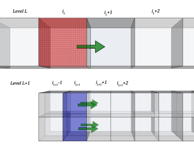
We will concentrate on the evolution of $D$ on a 3-dimensional spatial grid, though the remaining conserved fluid quantities are treated the same way, and modification to different numbers of spatial dimensions is trivial. Equation (3) is evolved numerically at a given resolution as

$$D^{n+1}_{i,j,k}=D^{n}_{i,j,k} -$$

$$\Delta t[(F^{x}_{i+1/2,j,k} - F^{x}_{i-1/2,j,k})/\Delta x$$

$$+(F^{y}_{i,j+1/2,k} - F^{y}_{i,j-1/2,k})/\Delta y$$

$$+(F^{z}_{i,j,k+1/2} - F^{z}_{i,j,k-1/2})/\Delta z]$$ (18)

where $D^{n}_{i,j,k}$ is the volume average of $D$ over the $(i,j,k)$ cell at time $t=n\Delta t$; $F^{x}_{i+1/2,j,k}$ is the flux $F^{x}=Dv^{x}$ through the $(i+1/2,j,k)$ cell face; $\Delta x$ is the $x$ length of each cell and so on for the $y$ and $z$ direction. In practice the flux values will be calculated with some HRSC technique combined with Runge-Kutta, but the specifics are not relevant here. Now consider a situation with two sequential levels of refinement, $L$ and $L+1$, where level $L+1$ has a higher resolution with spatial refinement ratio of $r$ in each direction, and its domain is a subset of level $L$. (In practice, we always take $r=2$.) Here we focus the discussion on a left boundary in the $x$ direction, as illustrated in Fig. 1; boundaries along the right face and other coordinate directions are treated in a like manner.

When evolving according to the Berger-Oliger algorithm, after each time step of length $\Delta t$ is taken on level $L$, $r$ steps of length $\Delta t/r$ are taken on level $L+1$. Then the results obtained on $L+1$ are injected into level $L$ where the levels overlap i.e., the restriction operation is performed conservatively by setting the value in the parent cell to the (coordinate) volume-weighted average of the child cells that make up the parent cell. Now on level $L$, the change in $D$ due to flux going through the cell face $(i_{L}+1/2,j_{L},k_{L})$ on a timestep will be

$$\delta D_{L}=-\frac{\Delta t}{\Delta x}F^{x}_{i_{L}+1/2,j_{L},k_{L}}(t_{n}).$$ (19)

On level $L+1$, the change in $D$ in one fine-level time step due to flux passing through one of the $r^{2}$ cell faces that make up this same interface is

$$\delta D_{L+1,j,k,m}=-\frac{\Delta t/r}{\Delta x/r}\times$$

$$F^{x}_{i_{L+1}+1/2,j_{L+1}+j,k_{L+1}+k}(t_{n}+m\Delta t/r).$$ (20)

for $j$, $k$, and $m\in\{0,1,\dots,r-1\}$. Now because of truncation error, in general the change in the net “mass” $\delta M_{L}:=\delta D_{L}V_{L}$ within the coarse-level cell at $(i_{L},j_{L},k_{L})$ computed with the coarse-level fluxes will not equal the corresponding quantity $\delta M_{L+1}:=\sum_{j,k,m}\delta D_{L+1,j,k,m}V_{L+1,j,k,m}$ computed with the fine-level fluxes, where $V_{L}$ is the coordinate volume of the cell $(i_{L},j_{L},k_{L})$ and $V_{L+1,j,k,m}$ is the coordinate volume of the cell $(i_{L+1},j_{L+1}+j,k_{L+1}+k)$. Thus, after the values of $D$ on level $L+1$ are injected into level $L$ (in cells $(i_{L}+1,j_{L},k_{L})$ and to the right in this example), the solution on level $L$ will suffer a violation of mass conservation proportional to $\delta M_{L}-\delta M_{L+1}$. To restore the conservative nature of the algorithm, the idea, described in detail below, is to adjust the conservative variable $D$ in the cell $(i_{L},j_{L},k_{L})$ post-injection by an amount to exactly compensate for this truncation error induced difference.

The scheme originally proposed in bc89 is to define an array that keeps track of a correction to the fluxes through cell faces on level $L$ that make up the boundary of the evolved cells on level $L+1$. Consider the case where $(i_{L}+1/2,j_{L},k_{L})$ is such a face. This face-centered flux correction array, $\delta F$, is initialized with the inverse of the flux in (19), $\delta F=-F^{x}_{i_{L}+1/2,j_{L}+j,k_{L}+k}$, and then during the course of taking the $r$ time steps on level $L+1$ receives corrections from the terms in (20)

$$\delta F\to\delta F+\frac{1}{r^{3}}\sum_{j,k,m}F^{x}_{i_{L+1}+1/2,j_{L+1}+j,k_{L+1}+k}(t_{n}+m\Delta t/r).$$ (21)

After the cell values on level $L$ are overwritten by the injected values on level $L+1$ where they overlap, the cells on level $L$ that abut level $L+1$ though are not themselves covered by level $L+1$ cells are corrected with the flux stored in $\delta F$.

The way we implement the flux correction algorithm is slightly different from this. In particular we wish to avoid the added computational complexity of implementing face-centered grid functions, and therefore we keep track of a cell-centered correction. The correction is thus also more naturally represented as a correction to the fluid quantity integrated within the volume of the cell (e.g. for $D$ the rest-mass) rather than a flux. Again referring to Fig. 1, we define the first few cells at the boundary of level $L+1$ as buffer cells since the calculation of flux requires knowledge of the state on both sides of the interface. These cells will have their values set by interpolation from those in level $L$. The innermost buffer cells for the boundary on level $L+1$ we call type B cells (blue cells in the lower half of the figure). These are the cells where the level $L+1$ contribution to the mass correction will be stored. The cell on level $L$ which contains the type B cell we will refer to as a type A cell (red, dotted-pattern cell). Type A cells are the ones that receive mass corrections in this algorithm. For each cell on each refinement level we use a bitmask grid function that indicates whether the cell is one of the above types (A or B), and if so which of the six possible faces ($+x$, $-x$, $+y$, $-y$, $+z$, $-z$) abut the boundary. For simplicity in the implementation we do not allow grid hierarchies where a cell would be both type A and type B.

In the following we outline the additional tasks relative to the basic Berger-Oliger algorithm that need to be performed with our implementation of Berger-Colella. Following the spirit of these algorithms, we break down the tasks into those the AMR “driver” code implements, which do not require knowledge of the specific equations being evolved or what physical quantities the variables represent, and conversely the “application” steps that would need to be implemented by a unigrid application code plugging into the driver to become AMR-capable. The driver tasks include the following:

1. For the conserved fluid density $D$, allocate a storage grid function to keep track of the associated mass correction $\delta M$, i.e. the total correction to $D$ within the volume of a given cell.

2. Upon initialization set all correction arrays $\delta M$ to zero, and compute the bitmask for the current refinement hierarchy.

3. After any regrid, recompute the bitmask array for the new hierarchy.

4. During the stage when buffer cells are set for variable $D$ at interior boundaries on level $L+1$ via interpolation from level $L$, also interpolate the correction variable $\delta M$, where the latter’s interpolation operator simply sets $\delta M$ in a child cell to be $1/r^{3}$ that of the parent cell (for a three-dimensional spatial grid).

5. Following injection of arrays $D$ and $\delta M$ from level $L+1$ to level $L$, where the injection operator for $\delta M$ is an algebraic sum over child cells (a) zero all type B cells in $\delta M$ on level $L+1$, (b) call the application routine (first item in the next list) to apply the mass corrections to $D$ stored in the injected $\delta M$ to type A cells on level $L$, (c) zero all type A cells in $\delta M$ on level $L$.

The following are new tasks that the unigrid application code needs to implement:

1. A routine that will add the mass corrections stored in $\delta M$ to $D$ for all type A cells on a given grid (i.e., set $D_{L}\rightarrow D_{L}+\delta M/V_{L}$).

2. When taking a single time step on a grid, for any cell marked type A, set $\delta M$ to minus the change in mass of the cell from fluxes through cell faces indicated by the bitmask. For example, with the case illustrated in Fig.1 and discussed above around Eqs. (19) and (20), set $\delta M_{L}=-V_{L}\delta D_{L}$.

3. When taking a single time step on a grid, for any cell marked type B, add to $\delta M$ the change in mass of the cell from fluxes through cell faces indicated by the bitmask. For example, with the same example above, set $\delta M_{L+1,j,k}\rightarrow\delta M_{L+1,j,k}+V_{L+1,j,k,m}\delta D_{L+1,j,k,m}$.

For the GR-hydro equations we have five conserved fluid variables, $D$ and $S_{a}$. Though the latter do have nonzero source terms — since gravity can be a source (or sink) of energy-momentum — the above algorithm ensures there will be no artificial loss/gain in the presence of AMR boundaries due to truncation error from the advection terms.

III Tests

In this section we present a number of tests of the methods presented above. We begin by demonstrating the fourth-order convergence of the evolution of the Einstein equations for vacuum spacetimes before moving on to a number of flat space, relativistic hydrodynamics tests that probe the treatment of fluid discontinuities. We conclude with several tests of hydrodynamics in curved spacetimes.

III.1 Vacuum evolution

In gh3d ; Pretorius:2006tp several tests of convergence of an earlier version of the code (without hydrodynamics) were presented. However, since then we have updated the evolution of the Einstein equations to fourth-order spatial differencing and fourth-order Runge-Kutta time differencing, so we first show two vacuum tests: a Brill wave evolution Brill ; Sorkin and a boosted BH evolution.

III.1.1 Brill wave

For the Brill wave test we begin with initial data where the spatial line element is given by

$$ds^{2}=\psi^{4}\Big{(}e^{B}dx^{2}+\frac{e^{B}y^{2}+z^{2}}{r^{2}}dy^{2}+$$

$$\frac{(e^{B}-1)yz}{r^{2}}(dydz+dzdy)+\frac{e^{B}z^{2}+y^{2}}{r^{2}}dz^{2}\Big{)}$$ (22)

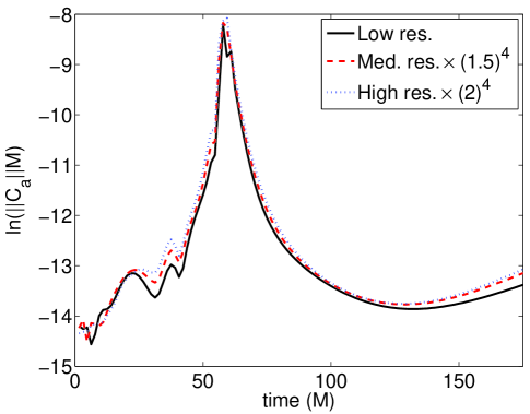
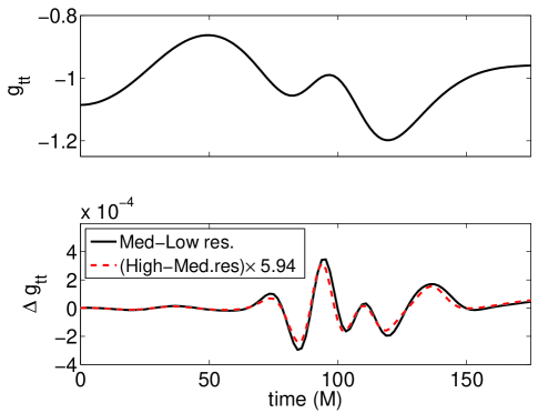
where $r=\sqrt{y^{2}+z^{2}}$, $B=2Ar^{2}\exp(-(r/\sigma_{r})^{2}-(x/\sigma_{x})^{2})$, and the value of the conformal factor $\Psi$ is determined by solving the Hamiltonian constraint. We choose $A=40$, $\sigma_{r}=0.16$, and $\sigma_{x}=0.12$. The initial data is chosen to be time symmetric ($\dot{\gamma}_{ij}=0$) and maximally sliced ($K=0$) with the conformal lapse $\tilde{\alpha}:=\Psi^{-6}\alpha=1$. The remaining metric components are chosen to satisfy the harmonic gauge ($\Box x^{a}=0$). This describes a gravitational wave that initially collapses inward before dispersing. In Fig. 2 we show results from convergence tests in axisymmetry at three resolutions where the medium and high runs had, respectively, 1.5 and 2 times the resolution of the low run. The constraint equations ($H_{a}-\Box x_{a}=0$) as well as the metric components show the expected fourth-order convergence.

Figure 2: Top: The natural log of the $L^{2}$ norm of the constraint violation, $C_{a}:=H_{a}-\Box x_{a}$, for a Brill wave evolution (i.e. natural log of $\sqrt{\int|C_{a}|^{2}d^{2}x/\int d^{2}x}$). The three resolutions shown are scaled assuming fourth-order convergence. Time is shown in units of $M$, the total ADM mass of the spacetime, and the constraints are multiplied by $M$ to make them dimensionless. The lowest resolution has a grid spacing of $h=1.56M$. Middle/Bottom: The value of the metric component $g_{tt}$ evaluated at $(x,y,z)=(0,50M,0)$ (middle) and the difference in this quantity between low and medium resolution, and medium and high resolution (bottom), the latter scaled so that the two curves should coincide for fourth-order convergence.

III.1.2 Boosted BH evolution

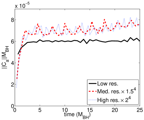
As an additional vacuum spacetime test we evolved a boosted BH in three dimensions. We began with initial data describing a BH in harmonic coordinates HarmonicBH with boost parameter $v=0.25$. As described in gh3d , during the evolution we avoid the BH singularity by searching for an apparent horizon and excising a region within. To demonstrate convergence we performed this simulation at three resolutions, the lowest of which has approximately 30 points covering the diameter of the BH. The medium (high) resolution has 1.5 (2.0) times the number of points in each dimension, respectively. For all resolutions we used the same AMR hierarchy, determined based on truncation error estimates at the lowest resolution, with six levels of 2:1 refinement. In Fig. 3 we demonstrate that the constraint equations are converging to zero at fourth-order. When hydrodynamics is included the theoretical limiting convergence rate of our code will drop to second-order (in the absence of shocks). However in vacuum dominated regions, for example the gravitational wave zone, one can expect that for the finite resolutions we can practically achieve the convergence will be somewhere between second- and fourth-order.

Figure 3: The $L^{2}$-norm of the constraint violation ($C_{a}:=H_{a}-\Box x_{a}$) in the equatorial plane for a boosted BH simulation with $v=0.25$. The three resolutions shown are scaled assuming fourth order convergence. Time is shown in units of $M_{\rm BH}$, the ADM mass of the BH in its rest frame, and the norm of the constraints is multiplied by $M_{\rm BH}$ so as to make it dimensionless.

III.2 Relativistic hydrodynamic tests in flat spacetime

We have performed a number of standard tests for relativistic, inviscid hydrodynamics that probe how well a given numerical scheme handles the various discontinuities that arise. The best combination of reconstruction and flux calculation methods depends on the problem under consideration. We have thus implemented several options and maintained a modular code infrastructure so that they are readily interchangeable and upgradable. While strong shocks such as the ones considered here are not expected to play an important dynamical role in binary BH-NS mergers, they might be important in other potential applications of interest (such as NS-NS grazing impacts, or understanding EM emission from collisions). Thus, the ability to tailor the reconstruction and flux methods to the problem at hand may prove important in the future. In this section, we closely follow the sequence of tests used in the development of the RAM code of Zhang and MacFadyen ramcode , so that our results may be compared with theirs. Though they focus on more sophisticated flux-reconstruction algorithms, their simpler methods (labeled U-PPM and U-PLM, denoting reconstruction of the unknowns with piecewise parabolic and linear reconstruction, respectively) are comparable to the ones we employ.

III.2.1 1D Riemann problems

Test	$\Gamma$a	$P_{L}$	$\rho_{L}$	$v_{L}$	$P_{R}$	$\rho_{R}$	$v_{R}$
RT1	5/3	13.33	10.0	0.0	$10^{-8}$	1.0	0.0
RT2	5/3	1000.0	1.0	0.0	$10^{-2}$	1.0	0.0
RT3	4/3	1.0	1.0	0.9	10.0	1.0	0.0
TVT	5/3	1000.0	1.0	0.0	1.0	1.0	$(0.0,0.99)$b

Table 1: The initial left and right states for the 1D Riemann problems.
^a Adiabatic index of EOS
^b In this case $v_{x}$=0 but the transverse velocity $v_{y}=0.99$ is nonzero.

Reconstruction	Flux method	RT1		RT2		RT3		TVT
		Errora	Convergenceb	Error	Convergence	Error	Convergence	Error	Convergence
MC	HLL	0.034	0.82	0.110	0.59	0.062	0.77	0.238	0.72
	Roe	0.032	0.82	0.110	0.60	0.052	0.80	0.233	0.72
	Marquina	0.036	0.82	0.127	0.59	0.056	0.79	0.227	0.76
Minmod	HLL	0.061	0.86	0.169	0.42	0.054	0.71	0.395	0.76
WENO5	HLL	0.033	0.84	0.093	0.76	0.039	0.61	0.191	0.83
	Roe	0.032	0.85	0.096	0.79	0.039	0.60	0.198	0.81
	Marquina	0.036	0.85	0.093	0.76	0.038	0.66	0.183	0.82
PPM	HLL	0.041	0.88	0.133	0.67	0.024	1.01	0.248	0.78

Table 2: 1D Riemann test results.
^aThe L1 norm of the error for resolution $N=400$.
^bThe average convergence rate between runs with $N=200,$ 400, 800, and 1600. The ideal rate is unity for problems such as these containing discontinuities.

We first present a series of four relativistic, one-dimensional (1D) Riemann problem tests for which the exact solution is known (see Sections 4.1-4.4 of ramcode ). In all cases, the domain is $x\in[0,1]$ and there are initially two fluid states, a left and a right, initially separated by an imaginary partition at $x=0.5$. At $t=0$, the partition is removed and the fluid evolves to some new state. A $\Gamma$-law EOS is used for all the tests. In Table 1 we summarize the initial states and adiabatic indices used for the four tests, which we label as RT1 (Riemann Test 1), RT2, RT3, and TVT (Transverse Velocity Test). We compare the performance of the various combinations of reconstruction schemes and flux methods to the exact solution and summarize the errors and convergence rates in Table 2. Exact solutions to these four tests were generated using a solver provided by B. Giacomazzo, which is described in bruno_code . Taking HLL as our basic flux method, we performed this series of Riemann problem tests with four reconstruction methods: MC, minmod, WENO5, and PPM. For MC and WENO5, we also explored the effect of the flux method by running the tests with the Roe solver and Marquina’s method. Most cases have a Courant-Friedrichs-Lewy (CFL) factor of 0.5. However, the Roe solver, when combined with WENO5, does not seem to work well for problems with very strong shocks, such as RT2 and TVT. For a CFL factor of 0.5, we obtain acceptable results with Roe only by using a more diffusive limiter (like MC). For RT2 and TVT, we thus use Roe combined with WENO5 with a CFL factor of 0.1.

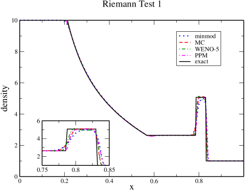
All of the methods we considered perform well on RT1, which is a fairly easy test. The lowest overall error occurs for WENO5 reconstruction (though the density profile between the shock and the contact discontinuity seems not to be as flat as in the other cases). The overall success of WENO5 may be due to the fact that the shock is relatively mild and there is an extended rarefaction that benefits from the high-order reconstruction. In Fig. 4 we compare the density profile obtained using HLL and various reconstruction methods to the exact solution. We note that the tests which used the Roe or Marquina flux calculation with WENO5 do not have the oscillation visible in the plot around $x=0.8$ in the HLL-WENO5 case.

Figure 4: Density at $t=0.4$ for Riemann Test 1 (RT1) with different reconstruction methods and the HLL flux scheme at resolution $N=400$. The inset shows the shock and contact discontinuity. The exact solution was generated using the code of bruno .

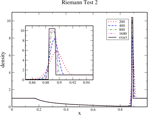
The second Riemann test (RT2) is more difficult than the first, with the blast wave resulting in a very thin shell of material bounded by a shock on the right and a contact discontinuity on the left (see Fig. 5). The average convergence rates for this test show a marked difference between the piecewise-linear and higher-order reconstruction methods. WENO5 seems to perform best, but there is not much difference between HLL and Marquina or the Roe solver (with diminished CFL factor) with WENO5. As in RT1, the reconstruction method seems to be more important to the solution than the flux scheme.

Figure 5: Density at $t=0.4$ for Riemann Test 2 (RT2) at different resolutions for HLL-WENO5. The average convergence rate in this case is 0.76. The thin shell of material between the shock and the contact is particularly difficult to resolve.

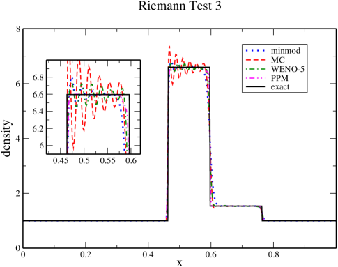
RT3 is a challenging problem in which the fluid on the left collides with the initially stationary fluid on the right, resulting in two shocks separated by a contact discontinuity. Our numerical solutions suffer from significant oscillations (particularly in the reverse shock) for all reconstruction schemes except PPM, which was specifically designed to suppress such post-shock oscillations (see Fig. 6). PPM also has the best convergence properties (0.85-1.16), with an average rate close to the expected value of unity. (Finite-volume hydrodynamic schemes such as this should converge at first order to a weak solution of the equations when discontinuities are present.)

Figure 6: Density at $t=0.4$ for Riemann Test 3 (RT3), a collision problem, for different reconstruction methods with HLL at resolution $N=400$. The post-shock oscillations are largest in the MC case and smallest for PPM.

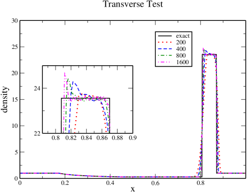
For the transverse velocity test, the initial data are set up as in RT2, except that there is a transverse velocity $v^{y}=0.99$ on the right side of the partition. The strong shock propagates into the boosted fluid, and the structure of the shock is altered, since the velocities in all directions are coupled through the Lorentz factor PhysRevLett.89.114501 . Again, the reconstruction technique influences the result more than the flux calculation. For WENO5 reconstruction, the errors for HLL, Roe, and Marquina are all very close in magnitude. WENO5 and PPM yield the best results overall. In Fig. 7 we show the density profile at different resolutions for HLL combined with WENO5.

Figure 7: Density at $t=0.4$ for the transverse test (TVT) at different resolutions for HLL-WENO5. The average convergence rate in this case is 0.83.

III.2.2 1D Shock-heating problem

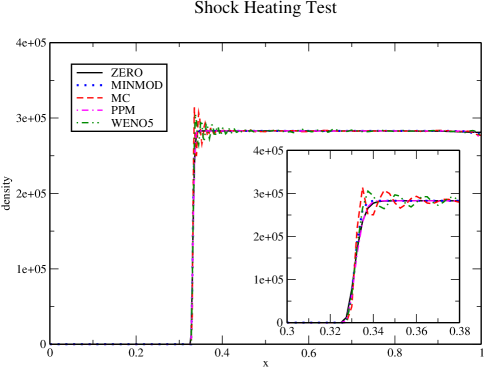
We next consider a one-dimensional shock-heating problem as in ramcode , which tests a code’s conservation of energy as well as the ability to handle strong shocks. For this problem, the computational domain is $x\in[0,1]$ with a reflecting boundary at $x=1$. The fluid moves toward this boundary with an ultrarelativistic initial velocity of $v=1-10^{-10}$. The fluid has an initial density of $\rho=1.0$ and a very small amount of specific internal energy, $\epsilon=0.003$. The EOS is a gamma-law with $\Gamma=4/3$. When the relativistic fluid slams into the wall, its kinetic energy is converted into internal energy behind a shock which propagates to the left. Because the fluid is initially cold, essentially all of the heat is generated through this conversion. As explained in ramcode , the shock speed and the compression ratio of the shock (or equivalently, the post-shock density) is known analytically. We evaluate our errors by calculating the L1 norm of the density errors on the entire computational domain. The average rate of convergence is also calculated using this measure of error.

We performed this test using HLL with five different reconstruction methods at four different resolutions (200, 400, 800, and 1600 zones). Results are shown in Table 3. We find that, due to the extremely strong shock, there is a tendency for post-shock oscillations to form with less diffusive reconstruction schemes (see Fig. 8). The WENO5 solution is afflicted with severe post-shock oscillations and exhibits poor convergence to the exact compression ratio. Very diffusive reconstruction schemes (zero slope and minmod) are comparatively quite successful and converge rapidly to the exact compression ratio. PPM, with its flattening step, gives the best convergence rate overall.

Reconstruction	Errora	Convergenceb
ZERO	950	0.94
Minmod	801	0.92
MC	1500	0.85
PPM	824	0.96
WENO5	1670	0.53

Table 3: Shock -heating test results. For this test we also compare to zero slope reconstruction, labeled “ZERO.”
^a The L1 norm of the error for resolution $N=400$.
^b The average convergence rate between runs with $N=200,$ 400, 800, and 1600.

Figure 8: Density at $t=2.0$ for the shock-heating test with different reconstruction methods and the HLL flux scheme. The inset focuses on the shock front.

III.2.3 Emery step problem

Next we consider the two-dimensional (2D) Emery step problem Emery ; ppm , with the setup as in ramcode . In this scenario, a fluid flows through a wind tunnel at relativistic speed and hits a step, which is represented by a reflecting boundary condition. The computational domain is $(x,y)\in[0,3]\times[0,1]-[0.6,3]\times[0,0.2]$ where the subtracted region represents the step. At the left boundary, inflow conditions are enforced (as in the initial data), while at the right, outflow conditions are enforced. All remaining boundaries are reflecting. The fluid is initialized with density $\rho=1.4$, velocity $v_{x}=0.999$, and a $\Gamma=1.4$ EOS. The pressure is set to 0.1534, giving a Newtonian Mach number of 3.0.

Higher-order reconstruction methods seem to be essential for this test problem. We find that the MC limiter performs poorly, regardless of the flux method. Although the MC simulation is stable, the bow shock formed as the fluid reflects off the step is distorted by large amplitude post-shock oscillations. These propagate downstream, rolling up the boundaries between the different solution regions. The higher resolution runs with MC also have these features, but at shorter wavelengths and lower amplitude. PPM and WENO5 reconstruction performs much better, and these results are shown at two resolutions in Fig. 9. (This figure can be compared to those of LucasSerrano:2004aq ; ramcode .) The PPM results appear slightly better than WENO5 at a given resolution, likely because of the deliberate oscillation suppression in the PPM algorithm.

Figure 9: Density contours (30 equally spaced in the logarithm) for the Emery step problem. The upper (lower) two plots show results for resolution $240\times 80$ ($480\times 160$). For each resolution, the upper plot shows results for WENO5 reconstruction, and the lower for PPM. The respective minimum and maximum densities, $(\rho_{\rm min},\rho_{\rm max})$, are $(1.0,1.0\times 10^{2})$, $(0.55,1.1\times 10^{2})$, $(0.82,1.1\times 10^{2})$, and $(6.8\times 10^{-2},1.1\times 10^{2})$.

III.2.4 2D shock tube problem

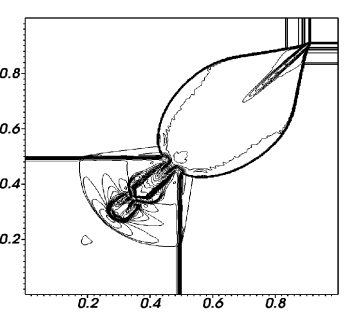
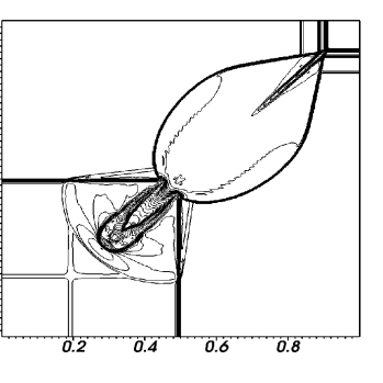
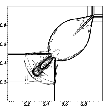
As an additional test of these algorithms’ ability to propagate strong, multidimensional shocks we consider a 2D shock tube test. The computational domain $(x,y)\in[0,1]\times[0,1]$ is divided into four equal quadrants. The initial fluid states in the lower/upper, left/right quadrants are

$$(\rho,P,v_{x},v_{y})^{LL} = (0.5,1,0,0)$$

$$(\rho,P,v_{x},v_{y})^{LR} = (0.1,1,0,0.99)$$

$$(\rho,P,v_{x},v_{y})^{UL} = (0.1,1,0.99,0)$$

$$(\rho,P,v_{x},v_{y})^{UR} = (0.1,0.01,0,0).$$

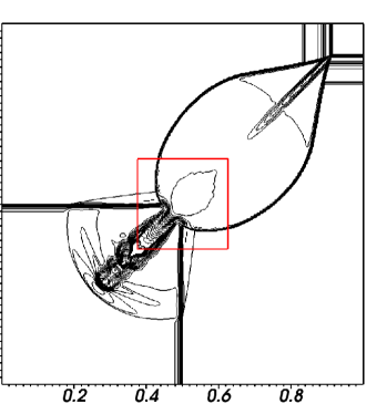
In this simulation the lower-right and upper-left quadrants converge on the upper-right quadrant creating a pair of curved shocks. We use a $\Gamma=5/3$ EOS. In Fig. 10 we show results from simulations using HLL or the Marquina flux method combined with WENO5 or the MC limiter. The first three panels are from runs with resolution of $400\times 400$ and a CFL factor of 0.5 and are comparable to ramcode and the references therein. Though the main shock features are captured by all of the methods we considered, oscillations arising from the curved shock fronts are evident in varying degrees. The fourth panel is similar to the first but contains a refined mesh in the center that has the same resolution as the other three panels, while the remainder of the domain has half the resolution. Though the majority of the flow is thus effectively derefined, the principal features remain the same. This is despite the fact that the shocks must travel through or along refinement boundaries, and the numerical shock speeds differ slightly on either side of such boundaries due to the different truncation errors.

Figure 10: Density contours (30 equally spaced in the logarithm) for the 2D Riemann problem with, from left to right, top to bottom: HLL and MC, HLL and WENO5, Marquina and MC, and HLL and MC with mesh refinement. The respective minimum and maximum densities, $(\rho_{\rm min},\rho_{\rm max})$, are $(1.1\times 10^{-2},7.0)$, $(8.2\times 10^{-3},8.1)$, $(9.1\times 10^{-3},7.1)$, and $(7.6\times 10^{-3},7.0)$. For the first three simulations a resolution of $400\times 400$ was used. For the final simulation, a refinement region (red box) was placed in the middle with equivalent resolution, while the remaining grid has half the resolution (i.e. this simulation has lower resolution overall). A CFL factor of 0.5 was used throughout.

III.3 Hydrodynamic tests in curved spacetime

III.3.1 Bondi accretion

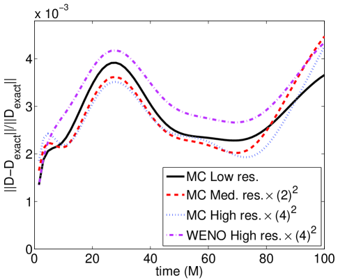
As a first test of our code’s ability to simulate relativistic hydrodynamics in the strong field regime, we consider Bondi flow. We set up our initial conditions with a stationary solution to spherical accretion onto a black hole ShapiroTeuk . We use Kerr-Schild coordinates for the black hole metric. In order to test our code’s ability to converge to the correct solution we measured how the conserved density $D$ differed from the exact solution as a function of time for three resolutions. The lowest resolution has a grid spacing of $h=0.078M_{BH}$, while the medium and high resolutions have twice and 4 times the resolution respectively. As shown in Fig. 11, $||D-D_{\rm exact}||$ converges to zero at second-order. For this test we tried both the MC and WENO5 limiters (with HLL for the flux calculation). Though both had similar levels of error and showed the expected convergence, WENO5 had larger errors at low and medium resolutions. This is probably because, at lower resolutions, the larger WENO5 stencil extends farther inside the black hole horizon where there is larger truncation error.

Figure 11: The $L^{2}$ norm of the difference between the numerical and exact value of the fluid quantity $D$ (divided by the norm of the exact solution) for Bondi accretion with MC and WENO5. The low resolution was run with a grid spacing of $h=0.078M_{BH}$ while the medium and high has twice and 4 times the resolution respectively. The results are scaled for second-order convergence.

III.3.2 Boosted NS

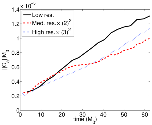
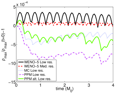
As an additional test of our evolution algorithm, we considered a single TOV star with a boost of $v=0.5$, with astrophysically relevant EOS (the HB EOS of jocelyn ) and mass (1.35 $M_{\odot}$). We performed a convergence study at three resolutions, the lowest of which has approximately 50 points covering the diameter of the star. The medium (high) resolution has two (three) times the number of points in each dimension, respectively. The AMR hierarchy is identical in all cases, with 7 levels of 2:1 refinement, and was determined using truncation error estimates from the low resolution run. Figure 12 shows that the constraint violations show the expected second-order convergence to zero. We also compared the performance of different reconstruction methods (though using the HLL flux method throughout). In Fig. 13, we show the maximum density of the NS as a function of time for various reconstruction methods. Though the drifts and oscillations in density converge away for all methods, we find that WENO5 gives the least density drift compared to MC and PPM at a given resolution. The drift in maximum density with PPM has to do with the way this particular implementation enforces monotonicity at extrema, which results in a loss of accuracy (see for example new_ppm ). Modifying the way the algorithm handles smooth extrema can reduce this effect. We implemented one such modification (Eqs. 20-23 from new_ppm ), the results of which are labeled ‘PPM alt.’ in Fig. 13.

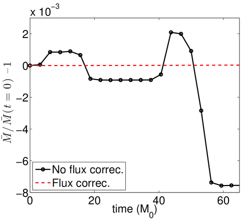
III.3.3 Boosted NS flux correction test

As a demonstration of the flux correction algorithm (outlined in Sec. II.4) to enforce conservation across AMR boundaries, we perform an additional boosted NS test. We use the same conditions as the low resolution simulation outlined above in Sec. III.3.2 but with a different AMR hierarchy. In particular, we keep the hierarchy fixed so that the boosted NS will move to areas of successively lower refinement. In Fig. 14, one sees that without flux corrections there is a $\approx 0.1\%$ loss in fluid rest-mass as the NS moves off the highest refinement level, and a $\approx 0.8\%$ loss as the NS moves off the next to highest refinement level. This change in the conserved fluid rest-mass comes from the fact that there is a slight mismatch in fluxes at the mesh refinement boundaries due to truncation error. With the flux correction routine activated, this error is eliminated, and the only change in the total rest-mass is due to the density floor criterion (i.e., the numerical atmosphere). As an indication of how the use of flux corrections affects energy and momentum we can also compare the integrated matter energy and momentum as seen by a set of Eulerian observers. The matter energy density is given by $T^{ab}n_{a}n_{b}$ and the momentum density is given by $p_{i}=-T^{a}_{i}n_{a}$ where $n_{a}$ is the timelike unit normal to the constant $t$ slices. These quantities involve combinations of the conserved fluid variables and the metric and are subject to truncation error, especially since in this simulation the NS is allowed to move to lower resolution. In addition, these quantities can vary with time due to gauge effects (though in this case, the variation due to gauge effects is subdominant to the variation mentioned below), so we use them as an indication of the effect of flux corrections by comparing them for the simulations with and without flux corrections to a similar simulation where the AMR tracks the NS and there is therefore essentially no flux across AMR boundaries. At the end of the simulation the run without flux corrections has $0.91\%$ less energy compared to a similar simulation where the AMR tracks the NS, while the run with flux corrections has only $0.13\%$ less energy. The run without flux corrections has $4.0\%$ less momentum (in the boost direction) while with flux corrections the comparative loss is $2.5\%$.

This test is somewhat artificial since we have deliberately prevented the AMR algorithm from tracking the NS. As long as the AMR algorithm can keep the boundaries away from areas of non-negligible flux (as it does when following the boosted NS in the test described in Sec. III.3.2) the effect of the flux correction algorithm is small, at the level of the numerical atmosphere that gets pulled along with the star. However, in astrophysical applications, situations may generically arise in which fluid crosses AMR boundaries. For example, the tidal tails formed by the disruption of a NS by a BH will cross refinement boundaries, and likewise for the subsequent accretion disk that forms, since it would be much too costly to keep these entire structures on the finest mesh. Of course, the hydrodynamic solution is still subject to truncation error, which could in principle affect aspects of the dynamics at the same order of magnitude as putative nonconservative effects. Though for certain problems, such as calculating the amount of unbound material following a BH-NS merger, or studying the late time accretion, it could be quite advantageous to ensure conservation within the hydrodynamic sector. It would be an interesting computational science problem to systematically study the efficacy of AMR boundary flux conservation in such scenarios.

Figure 12: The $L^{2}$-norm of the constraint violation ($C_{a}:=H_{a}-\Box x_{a}$) in the equatorial plane for a boosted NS simulation with $v=0.5$ (using HLL flux calculation and WENO5 limiter). The three resolutions shown are scaled assuming second-order convergence. Time is shown in units of $M_{0}$, the ADM mass of the NS in its rest frame, and the norm of the constraints is multiplied by $M_{0}$ so as to make it dimensionless.

Figure 13: The relative variation of the maximum central density from its initial value ($\rho_{\rm max}/\rho_{\rm max}(t=0)-1$) during a boosted NS simulation with $v=0.5$ for various reconstruction methods and for two different resolutions in the case of WENO5.

Figure 14: The relative variation of the fluid rest-mass ($\bar{M}/\bar{M}(t=0)-1$) for a boosted NS test with (dotted, red line) and without (solid black line) flux corrections at mesh refinement boundaries. For this test, the mesh hierarchy is fixed so that at $t\approx$ 20 $M_{0}$ the NS has moved from being contained entirely on the finest resolution to being contained entirely on the second finest resolution. At $t\approx$ 60 $M_{0}$ the NS has moved from the second to the third finest resolution.

Finally, we note that additional convergence test results from this code were presented in ebhns_paper for the particular BH-NS merger simulations discussed there.

IV Conclusions

Numerous scenarios that fall within the purview of general relativistic hydrodynamics are still mostly unexplored—especially CO mergers involving neutron stars. There is a rich parameter space, of which large areas remain uncharted due to uncertainty or potential variability in BH and NS masses, BH spin and alignment, the NS EOS, and other aspects. Beyond the pure hydrodynamics problem, the roles of magnetic fields and neutrino physics are just beginning to be explored by various groups, and we expect to add support for such physics to our code in the future. The potential applications of robust and flexible numerical algorithms for evolving hydrodynamics together with the Einstein field equations are manifold. With this in mind, we have implemented methods for conservatively evolving arbitrary EOSs, in particular for converting from conserved to primitive variables without knowledge of derivatives; and we have implemented numerous reconstruction and flux calculation methods that can be used interchangeably to meet problem specific requirements. Though accurate treatment of shocks may not be crucial for BH-NS mergers (where shocks are not expected to be dynamically important), the same is not true of NS-NS binaries, especially eccentric ones where the stars may come into contact during nonmerger close encounters Roman . We have also taken care to implement a flux correction algorithm that preserves the conservative nature of hydrodynamical advection across AMR boundaries. Though strict conservation is not, strictly speaking, essential (since any nonconservation would be at the level of truncation error), it is an especially appealing property when studying, for example, CO mergers as potential SGRB progenitors. After merger, material that did not fall into the black hole — typically on the order of a few percent of the original NS mass — will fill a large volume making up an accretion disk and potentially unbound material. Though accurately tracking this material is not important for the gravitational dynamics, it is critical for characterizing potential EM counterparts to the merger.

Appendix A Spectral decomposition of the flux Jacobian

Our conservative formulation of the hydrodynamical equations (3,4) can be written in vector notation as $\partial_{t}\mathbf{q}+\partial_{i}(\mathbf{F}^{i})=\mathbf{S}$ where $\mathbf{q}$ is a five dimensional vector of the conserved (in the absence of sources $\mathbf{S}$) fluid variables $\mathbf{q}=(D,S_{t},S_{x},S_{y},S_{z})^{T}$ and the flux $\mathbf{F}^{i}=(Dv^{i},(S_{t}-\sqrt{-g}P)v^{i},S_{j}v^{i}+\delta_{j}^{i}\sqrt{-g}P)^{T}$, where the index $j$ in the flux is shorthand for the 3 components $(x,y,z)$. Some flux calculation methods such as the Roe solver eulderink and the Marquina flux marquinaFlux require the spectral decomposition of the Jacobian $\frac{\partial\mathbf{F}^{i}}{\partial\mathbf{q}}$ which we give here. (See flux_spec for the spectral decomposition for a similar formulation with slightly different conserved variables.) The eigenvalues are

$$\lambda_{\pm}=\alpha q(a\pm b)-\beta^{i}$$ (23)

and

$$\lambda_{3}=\alpha U^{i}-\beta^{i}$$ (24)

(with multiplicity 3), where $a=(1-c_{s}^{2})U^{i}$, $b=c_{s}\sqrt{(1-U^{2})[\gamma^{ii}(1-U^{2}c_{s}^{2})-aU^{i}]}$, $q=(1-U^{2}c_{s}^{2})^{-1}$, $c_{s}$ is the sound speed, and $\alpha,\beta^{i},\gamma^{ij}$ are metric components as in (10). Here and throughout we use $i\in\{x,y,z\}$ to refer to the direction of the flux in the Jacobian with which we are concerned, $\frac{\partial\mathbf{F}^{i}}{\partial\mathbf{q}}$. In the following equations we use the index $j$ as a shorthand for the three spatial components of the eigenvectors (that is, the components associated with $S_{x}$, $S_{y}$, and $S_{z}$). The indices $l$ and $m$ are fixed by $i$ and the indices $n$ and $p$ are fixed by $j$ as indicated below. The index $k$ is the only index that is summed over. A set of linearly independent right eigenvectors is given by

$$\mathbf{r}_{\pm}=\Big{(}1,hW[U^{k}\beta_{k}-\{\alpha(\gamma^{ii}-U^{i}U^{i})+A\beta^{i}\}/B],hW(U_{j}-\delta^{i}_{j}A/B)\Big{)}^{T},$$ (25)

where $A=[U^{i}c_{s}^{2}(1-U^{2})\mp b]q$ and $B=\gamma^{ii}-U^{i}(a\pm b)q$,

$$\mathbf{r}_{3}=\Big{(}\kappa/(HW(\kappa/\rho-c_{s}^{2})),U_{k}\beta^{k}-\alpha,U_{j}\Big{)}^{T},$$ (26)

where $\kappa=\frac{\partial P}{\partial\epsilon}$, and,

$$\mathbf{r}_{4}=\Big{(}WU_{l},2hW^{2}(U_{k}\beta^{k}-\alpha)U_{l}+h\beta_{l},h(\gamma_{jl}+2W^{2}U_{j}U_{l})\Big{)}^{T}$$ (27)

where for $\mathbf{r}_{4}$, $l=y,z,x$ for $i=x,y,z$ respectively. The expression for $\mathbf{r}_{5}$ can be obtained simply by replacing $l$ with $m$, where $m=z,x,y$ for $i=x,y,z$ respectively, in the above expression for $\mathbf{r}_{4}$. $H$ and $W$ are as defined following (12).

We also give the corresponding left eigenvectors. Component-wise, for $\mathbf{l}_{\pm}=(l^{D}_{\pm},l^{t}_{\pm},l^{j}_{\pm})$,

$$l^{D}_{\pm} = \mp fhWV_{\mp}\xi$$

$$l^{t}_{\pm} = \mp f\Big{[}(K-1)\{-\gamma U^{i}+V_{\mp}(W^{2}\xi-\Gamma_{lm})\}+KW^{2}V_{\mp}\xi\Big{]}/\alpha$$

$$l^{j}_{\pm} = \mp f\Big{[}(\gamma_{ln}\gamma_{mp}-\gamma_{lp}\gamma_{mn})\{1-KA^{i}-(2K-1)V_{\mp}U^{i}\}+(2K-1)V_{\mp}\xi W^{2}U^{j}\Big{]}-\beta^{j}l^{t}_{\pm}$$ (28)

where $l=y,z,x$ and $m=z,x,y$ for $i=x,y,z$ respectively, and $n=y,z,x$ and $p=z,x,y$ for $j=x,y,z$ respectively and $\Gamma_{lm}=\gamma_{ll}\gamma_{mm}-\gamma_{lm}\gamma_{lm}$, $\xi=\Gamma_{lm}-\gamma U^{i}U^{i}$, $K=(1-c_{s}^{2}\rho/\kappa)^{-1}$, $\Lambda_{\pm}=(a\pm b)q$, $V_{\pm}=(U^{i}-\Lambda_{\pm})/(\gamma^{ii}-U^{i}\Lambda_{\pm})$, $A^{i}=(\gamma^{ii}-U^{i}U^{i})/(\gamma^{ii}-U^{i}\Lambda_{\mp})$, and

$$f^{-1} = 2hWbq\xi(K-1)(\gamma^{ii}-U^{i}U^{i})\times$$

$$[(\gamma^{ii}-U^{i}\Lambda_{+})(\gamma^{ii}-U^{i}\Lambda_{-})]^{-1}.$$

Furthermore,

$$\mathbf{l}_{3}=\frac{W}{c_{s}^{2}\rho}(\kappa-c_{s}^{2}\rho)\Big{(}h,W/\alpha,W(U^{j}-\beta^{j}/\alpha)\Big{)},$$ (29)

and the components of $\mathbf{l}_{4}$ and $\mathbf{l}_{5}$ are

$$l^{D}_{4} = 0$$

$$l^{t}_{4} = G_{lm}(\alpha h\xi)^{-1}$$

$$l^{j}_{4} = \Big{[}\delta_{i}^{j}U^{i}G_{lm}+\delta_{l}^{j}\{\gamma_{mm}(1-U_{i}U^{i})+\gamma_{im}U_{m}U^{i}\}$$

$$-\delta_{m}^{j}\{\gamma_{lm}(1-U_{i}U^{i})+\gamma_{im}U_{l}U^{i}\}\Big{]}(h\xi)^{-1}$$

$$-\beta^{j}l^{t}_{4}$$ (30)

where $G_{lm}=(\gamma_{mm}U_{l}-\gamma_{lm}U_{m})$ and for $\mathbf{l}_{4}$, $l=y,z,x$ and $m=z,x,y$ for $i=x,y,z$ respectively. The expression for $\mathbf{l}_{5}$ can be obtained from the above expression for $\mathbf{l}_{4}$ simply by interchanging $l$ and $m$.

References

- [1] A. Abramovici et al. Ligo: The laser interferometer gravitational wave observatory. Science, 256:325, 1992.
- [2] H. Lück et al. The geo-600 project. Class. and Quant. Grav., 15:1471, 1997.
- [3] M. Ando et al. Stable operation of a 300-m laser interferometer with sufficient sensitivity to detect gravitational-wave events within our galaxy. Phys. Rev. Lett. , 86:3950, 2001. astro-ph/0105473.
- [4] B. Caron et al. The virgo interferometer. Class. and Quant. Grav., 14:1461, 1997.
- [5] Ramesh Narayan, Bohdan Paczynski, and Tsvi Piran. Gamma-ray bursts as the death throes of massive binary stars. Astrophys. J. , 395:L83, 1992. astro-ph/9204001.
- [6] N. Gehrels et al. A short -ray burst apparently associated with an elliptical galaxy at redshift z = 0.225. Nature (London), 437:851–854, October 2005.
- [7] W. H. Lee, E. Ramirez-Ruiz, and J. Granot. A Compact Binary Merger Model for the Short, Hard GRB 050509b. Astrophys. J. Lett., 630:L165–L168, September 2005.
- [8] B. D. Metzger and E. Berger. What is the Most Promising Electromagnetic Counterpart of a Neutron Star Binary Merger? ArXiv e-prints, August 2011.
- [9] M. Branchesi, on behalf of the LIGO Scientific Collaboration, the Virgo Collaboration, A. Klotz, and M. Laas-Bourez. Searching for electromagnetic counterparts of gravitational wave transients. ArXiv e-prints, October 2011.
- [10] The LIGO Scientific Collaboration, Virgo Collaboration: J. Abadie, B. P. Abbott, R. Abbott, T. D. Abbott, M. Abernathy, T. Accadia, F. Acernese, C. Adams, R. Adhikari, and et al. Implementation and testing of the first prompt search for electromagnetic counterparts to gravitational wave transients. ArXiv e-prints, September 2011.
- [11] N.K. Glendenning. Compact Stars: : Nuclear Physics, Particle Physics, and General Relativity. Springer, Berlin, Germany, 2000.
- [12] Y. Sekiguchi, K. Kiuchi, K. Kyutoku, and M. Shibata. Effects of hyperons in binary neutron star mergers. ArXiv e-prints, October 2011.
- [13] F. Pannarale, L. Rezzolla, F. Ohme, and J. S. Read. Will black hole-neutron star binary inspirals tell us about the neutron star equation of state? ArXiv e-prints, March 2011.
- [14] J. S. Read, C. Markakis, M. Shibata, K. Uryū, J. D. E. Creighton, and J. L. Friedman. Measuring the neutron star equation of state with gravitational wave observations. Phys. Rev. D, 79(12):124033, 2009.
- [15] R. Oechslin and H.-T. Janka. Gravitational Waves from Relativistic Neutron-Star Mergers with Microphysical Equations of State. Phys. Rev. Lett. , 99(12):121102, 2007.
- [16] L. K. Tsui, P. T. Leung, and J. Wu. Determination of the internal structure of neutron stars from gravitational wave spectra. Phys. Rev. D, 74(12):124025, 2006.
- [17] K. D. Kokkotas and N. Stergioulas. Gravitational Waves from Compact Sources. In A. M. Mourão, M. Pimenta, R. Potting, & P. M. Sá , editor, New Worlds in Astroparticle Physics: Proceedings of the Fifth International Workshop, page 25, 2006.
- [18] M. Shibata. Constraining Nuclear Equations of State Using Gravitational Waves from Hypermassive Neutron Stars. Phys. Rev. Lett. , 94(20):201101, 2005.
- [19] M. Shibata, K. Taniguchi, and K. Uryū. Merger of binary neutron stars with realistic equations of state in full general relativity. Phys. Rev. D, 71(8):084021, 2005.
- [20] J. Faber, P. Grandclément, and F. Rasio. Relativistic calculations of coalescing binary neutron stars. Pramana, 63:837, 2004.
- [21] M. Bejger, D. Gondek-Rosińska, E. Gourgoulhon, P. Haensel, K. Taniguchi, and J. L. Zdunik. Impact of the nuclear equation of state on the last orbits of binary neutron stars. Astron. and Astrophys., 431:297, 2005.
- [22] D. Lai and A. G. Wiseman. Innermost stable circular orbit of inspiraling neutron-star binaries: Tidal effects, post-Newtonian effects, and the neutron-star equation of state. Phys. Rev. D, 54:3958, 1996.
- [23] X. Zhuge, J. M. Centrella, and S. L. W. McMillan. Gravitational radiation from coalescing binary neutron stars. Phys. Rev. D, 50:6247, 1994.
- [24] P. J. Montero, O. Zanotti, J. A. Font, and L. Rezzolla. Dynamics of magnetized relativistic tori oscillating around black holes. Mon. Not. Roy. Astron. Soc., 378:1101–1110, July 2007.
- [25] O. Korobkin, E. B. Abdikamalov, E. Schnetter, N. Stergioulas, and B. Zink. Stability of general-relativistic accretion disks. Phys. Rev. D, 83(4):043007, February 2011.
- [26] B. D. Farris, Y. T. Liu, and S. L. Shapiro. Binary black hole mergers in gaseous disks: Simulations in general relativity. Phys. Rev. D, 84(2):024024, July 2011.
- [27] T. Bode, T. Bogdanović, R. Haas, J. Healy, P. Laguna, and D. Shoemaker. Mergers of Supermassive Black Holes in Astrophysical Environments. Astrophys. J. , 744:45, January 2012.
- [28] V. Paschalidis, Y. T. Liu, Z. Etienne, and S. L. Shapiro. Merger of binary white dwarf–neutron stars: Simulations in full general relativity. Phys. Rev. D, 84(10):104032, November 2011.
- [29] Jos A. Font. Numerical hydrodynamics and magnetohydrodynamics in general relativity. Living Reviews in Relativity, 11(7), 2008.
- [30] B. Zink, E. Schnetter, and M. Tiglio. Multipatch methods in general relativistic astrophysics: Hydrodynamical flows on fixed backgrounds. Phys. Rev. D, 77(10):103015, May 2008.
- [31] B. Zink. HORIZON: Accelerated General Relativistic Magnetohydrodynamics. ArXiv e-prints, February 2011.
- [32] M. D. Duez, Y. T. Liu, S. L. Shapiro, and B. C. Stephens. Relativistic magnetohydrodynamics in dynamical spacetimes: Numerical methods and tests. Phys. Rev. D, 72(2):024028, 2005.
- [33] Tetsuro Yamamoto, Masaru Shibata, and Keisuke Taniguchi. Simulating coalescing compact binaries by a new code (sacra). Phys. Rev. D, 78:064054, Sep 2008.
- [34] B. Giacomazzo and L. Rezzolla. WhiskyMHD: a new numerical code for general relativistic magnetohydrodynamics. Class. and Quant. Grav., 24:235, 2007.
- [35] M. Thierfelder, S. Bernuzzi, and B. Brügmann. Numerical relativity simulations of binary neutron stars. Phys. Rev. D, 84(4):044012, August 2011.
- [36] Tanja Bode, Roland Haas, Tamara Bogdanovic, Pablo Laguna, and Deirdre Shoemaker. Relativistic Mergers of Supermassive Black Holes and their Electromagnetic Signatures. Astrophys.J., 715:1117–1131, 2010.
- [37] M. Shibata and T. Nakamura. Evolution of three-dimensional gravitational waves: Harmonic slicing case. Phys. Rev. D, 52:5428, 1995.
- [38] T. W. Baumgarte and S. L. Shapiro. Numerical integration of Einstein’s field equations. Phys. Rev. D, 59(2):024007, 1999.
- [39] M. D. Duez, F. Foucart, L. E. Kidder, H. P. Pfeiffer, M. A. Scheel, and S. A. Teukolsky. Evolving black hole-neutron star binaries in general relativity using pseudospectral and finite difference methods. Phys. Rev. D, 78(10):104015, 2008.
- [40] M. Anderson, E. W. Hirschmann, S. L. Liebling, and D. Neilsen. Relativistic MHD with adaptive mesh refinement. Class. and Quant. Grav., 23:6503, 2006.
- [41] D. Garfinkle. Harmonic coordinate method for simulating generic singularities. Phys. Rev. D, 65(4):044029, 2002.
- [42] F. Pretorius. Numerical relativity using a generalized harmonic decomposition. Class. and Quant. Grav., 22:425, 2005.
- [43] L. Lindblom, M. A. Scheel, L. E. Kidder, R. Owen, and O. Rinne. A new generalized harmonic evolution system. Class. and Quant. Grav., 23:447, 2006.
- [44] S. Chawla, M. Anderson, M. Besselman, L. Lehner, S. L. Liebling, P. M. Motl, and D. Neilsen. Mergers of Magnetized Neutron Stars with Spinning Black Holes: Disruption, Accretion, and Fallback. Phys. Rev. Lett. , 105(11):111101–+, September 2010.
- [45] Z. B. Etienne, Y. T. Liu, and S. L. Shapiro. Relativistic magnetohydrodynamics in dynamical spacetimes: A new adaptive mesh refinement implementation. Phys. Rev. D, 82(8):084031, October 2010.
- [46] Z. B. Etienne, V. Paschalidis, Y. T. Liu, and S. L. Shapiro. Relativistic MHD in dynamical spacetimes: Improved EM gauge condition for AMR grids. ArXiv e-prints, October 2011.
- [47] Luis Lehner, Carlos Palenzuela, Steven L. Liebling, Christopher Thompson, and Chad Hanna. Intense Electromagnetic Outbursts from Collapsing Hypermassive Neutron Stars. 2011.
- [48] M. D. Duez, F. Foucart, L. E. Kidder, C. D. Ott, and S. A. Teukolsky. Equation of state effects in black hole-neutron star mergers. Classical and Quantum Gravity, 27(11):114106–+, June 2010.
- [49] K. Kiuchi, Y. Sekiguchi, M. Shibata, and K. Taniguchi. Exploring Binary-Neutron-Star-Merger Scenario of Short-Gamma-Ray Bursts by Gravitational-Wave Observation. Phys. Rev. Lett. , 104(14):141101, April 2010.
- [50] K. Kyutoku, H. Okawa, M. Shibata, and K. Taniguchi. Gravitational waves from spinning black hole-neutron star binaries: dependence on black hole spins and on neutron star equations of state. Phys. Rev. D, 84(6):064018, September 2011.
- [51] V. Paschalidis, Z. Etienne, Y. T. Liu, and S. L. Shapiro. Head-on collisions of binary white dwarf-neutron stars: Simulations in full general relativity. Phys. Rev. D, 83(6):064002, March 2011.
- [52] Y. Sekiguchi, K. Kiuchi, K. Kyutoku, and M. Shibata. Gravitational Waves and Neutrino Emission from the Merger of Binary Neutron Stars. Phys. Rev. Lett. , 107(5):051102, July 2011.
- [53] M. Shibata, K. Kiuchi, Y. Sekiguchi, and Y. Suwa. Truncated Moment Formalism for Radiation Hydrodynamics in Numerical Relativity. Prog. Theor. Phys., 125:1255–1287, June 2011.
- [54] B. Müller, H.-T. Janka, and H. Dimmelmeier. A New Multi-dimensional General Relativistic Neutrino Hydrodynamic Code for Core-collapse Supernovae. I. Method and Code Tests in Spherical Symmetry. Astrophys. J. Supp., 189:104–133, July 2010.
- [55] P. Cerdá-Durán, J. A. Font, L. Antón, and E. Müller. A new general relativistic magnetohydrodynamics code for dynamical spacetimes. Astron. and Astrophys., 492:937–953, December 2008.
- [56] W. H. Lee and W. Kluźniak. Newtonian Hydrodynamics of the Coalescence of Black Holes with Neutron Stars. I. Tidally Locked Binaries with a Stiff Equation of State. Astrophys. J. , 526:178–199, November 1999.
- [57] S. Rosswog and D. Price. MAGMA: a three-dimensional, Lagrangian magnetohydrodynamics code for merger applications. Mon. Not. Roy. Astron. Soc., 379:915–931, August 2007.
- [58] J. A. Faber, P. Grandclément, and F. A. Rasio. Mergers of irrotational neutron star binaries in conformally flat gravity. Phys. Rev. D, 69(12):124036, June 2004.
- [59] R. Oechslin, H.-T. Janka, and A. Marek. Relativistic neutron star merger simulations with non-zero temperature equations of state. I. Variation of binary parameters and equation of state. Astron. and Astrophys., 467:395–409, May 2007.
- [60] P. Laguna, W. A. Miller, and W. H. Zurek. Smoothed particle hydrodynamics near a black hole. Astrophys. J. , 404:678–685, February 1993.
- [61] S. Rosswog. Conservative, special-relativistic smoothed particle hydrodynamics. Journal of Computational Physics, 229:8591–8612, November 2010.
- [62] M.J. Berger and P. Colella. Local adaptive mesh refinement for shock hydrodynamics. Journal of Computational Physics, 82(1):64, 1989.
- [63] J. M. Stone, T. A. Gardiner, P. Teuben, J. F. Hawley, and J. B. Simon. Athena: A New Code for Astrophysical MHD. Astrophys. J. Supp., 178:137, 2008.
- [64] A. S. Almgren, V. E. Beckner, J. B. Bell, M. S. Day, L. H. Howell, C. C. Joggerst, M. J. Lijewski, A. Nonaka, M. Singer, and M. Zingale. CASTRO: A New Compressible Astrophysical Solver. I. Hydrodynamics and Self-gravity. Astrophys. J. , 715:1221–1238, June 2010.
- [65] D. C. Collins, H. Xu, M. L. Norman, H. Li, and S. Li. Cosmological Adaptive Mesh Refinement Magnetohydrodynamics with Enzo. Astrophys. J. Supp., 186:308–333, February 2010.
- [66] B. Fryxell, K. Olson, P. Ricker, F. X. Timmes, M. Zingale, D. Q. Lamb, P. MacNeice, R. Rosner, J. W. Truran, and H. Tufo. FLASH: An Adaptive Mesh Hydrodynamics Code for Modeling Astrophysical Thermonuclear Flashes. Astrophys. J. Supp., 131:273–334, November 2000.
- [67] K. Beckwith and J. M. Stone. A Second-order Godunov Method for Multi-dimensional Relativistic Magnetohydrodynamics. Astrophys. J. Supp., 193:6, March 2011.
- [68] Branson C. Stephens, William E. East, and Frans Pretorius. Eccentric Black Hole-Neutron Star Mergers. Astrophys. J. Lett., 737(1):L5, 2011.
- [69] W. E. East, F. Pretorius, and B. C. Stephens. Eccentric black hole-neutron star mergers: effects of black hole spin and equation of state. ArXiv e-prints, November 2011.
- [70] Helmut Friedrich. On the hyperbolicity of einstein’s and other gauge field equations. Communications in Mathematical Physics, 100:525–543, 1985. 10.1007/BF01217728.
- [71] Carsten Gundlach, Jose M. Martin-Garcia, Gioel Calabrese, and Ian Hinder. Constraint damping in the Z4 formulation and harmonic gauge. Class. Quant. Grav., 22:3767–3774, 2005.
- [72] F. Pretorius. Evolution of Binary Black-Hole Spacetimes. Phys. Rev. Lett. , 95(12):121101, 2005.
- [73] José A. Font, Mark Miller, Wai-Mo Suen, and Malcolm Tobias. Three-dimensional numerical general relativistic hydrodynamics: Formulations, methods, and code tests. Phys. Rev. D, 61:044011, Jan 2000.
- [74] C. F. Gammie, J. C. McKinney, and G. Tóth. HARM: A Numerical Scheme for General Relativistic Magnetohydrodynamics. Astrophys. J. , 589:444–457, May 2003.
- [75] Miguel Alcubierre, Steven Brandt, Bernd Bruegmann, Daniel Holz, Edward Seidel, et al. Symmetry without symmetry: Numerical simulation of axisymmetric systems using Cartesian grids. Int.J.Mod.Phys., D10:273–290, 2001.
- [76] A. Harten, P.D. Lax, and B.J. van Leer. SIAM Rev., 25:35, 1983.
- [77] F. Eulderink and G. Mellema. General relativistic hydrodynamics with a ROE solver. Astron. and Astrophys. Supp., 110:587, 1995.
- [78] R. Donat and A. Marquina. Capturing shock reflections: An improved flux formula. J. Comput. Phys., 125:42–58, 1996.
- [79] Chi-Wang Shu and Stanley Osher. Efficient implementation of essentially non-oscillatory shock-capturing schemes, ii. Journal of Computational Physics, 83(1):32 – 78, 1989.
- [80] E.F. Toro. Riemann Solvers and Numerical Methods for Fluid Dynamics. Springer, Berlin, Germany, 1997.
- [81] P. Colella and P. R. Woodward. The Piecewise Parabolic Method (PPM) for Gas-Dynamical Simulations. Journal of Computational Physics, 54:174, 1984.
- [82] José Ma Martí and Ewald Müller. Extension of the piecewise parabolic method to one-dimensional relativistic hydrodynamics. Journal of Computational Physics, 123(1):1 – 14, 1996.
- [83] Guang-Shan Jiang and Chi-Wang Shu. Efficient implementation of weighted eno schemes. Journal of Computational Physics, 126(1):202 – 228, 1996.
- [84] A. Tchekhovskoy, J. C. McKinney, and R. Narayan. WHAM: a WENO-based general relativistic numerical scheme - I. Hydrodynamics. Mon. Not. Roy. Astron. Soc., 379:469, 2007.
- [85] Scott C. Noble and Matthew W. Choptuik. Type ii critical phenomena of neutron star collapse. Phys. Rev. D, 78:064059, Sep 2008.
- [86] H. Shen, H. Toki, K. Oyamatsu, and K. Sumiyoshi. Relativistic equation of state of nuclear matter for supernova and neutron star. Nuclear Physics A, 637:435, 1998.
- [87] H. Shen, H. Toki, K. Oyamatsu, and K. Sumiyoshi. Relativistic Equation of State of Nuclear Matter for Supernova Explosion. Progress of Theoretical Physics, 100:1013, 1998.
- [88] R.P. Brent. Algorithms for minimization without derivatives. Prentice-Hall, Englewood Cliffs, N.J., 1972.
- [89] Marsha J Berger and Joseph Oliger. Adaptive mesh refinement for hyperbolic partial differential equations. Journal of Computational Physics, 53(3):484, 1984.
- [90] F. Pretorius and M. W. Choptuik. Adaptive mesh refinement for coupled elliptic-hyperbolic systems. Journal of Computational Physics, 218:246–274, October 2006.
- [91] Frans Pretorius. Simulation of binary black hole spacetimes with a harmonic evolution scheme. Class.Quant.Grav., 23:S529–S552, 2006.
- [92] Dieter R. Brill. On the positive definite mass of the bondi-weber-wheeler time-symmetric gravitational waves. Annals of Physics, 7(4):466 – 483, 1959.
- [93] Evgeny Sorkin. On critical collapse of gravitational waves. Classical and Quantum Gravity, 28(2):025011, 2011.
- [94] Gregory B. Cook and Mark A. Scheel. Well-behaved harmonic time slices of a charged, rotating, boosted black hole. Phys. Rev. D, 56:4775–4781, Oct 1997.
- [95] W. Zhang and A. I. MacFadyen. RAM: A Relativistic Adaptive Mesh Refinement Hydrodynamics Code. Astrophys. J. Supp., 164:255, 2006.
- [96] B. Giacomazzo and L. Rezzolla. The exact solution of the Riemann problem in relativistic magnetohydrodynamics. Journal of Fluid Mechanics, 562:223–259, September 2006.
- [97] B. Giacomazzo, L. Rezzolla, and L. Baiotti. Can magnetic fields be detected during the inspiral of binary neutron stars? Mon. Not. Roy. Astron. Soc., 399:L164, 2009.
- [98] Luciano Rezzolla and Olindo Zanotti. New relativistic effects in the dynamics of nonlinear hydrodynamical waves. Phys. Rev. Lett., 89:114501, Aug 2002.
- [99] Ashley F. Emery. An evaluation of several differencing methods for inviscid fluid flow problems. Journal of Computational Physics, 2(3):306 – 331, 1968.
- [100] Arturo Lucas-Serrano, Jose A. Font, Jose M. Ibanez, and Jose M. Marti. Assessment of a high-resolution central scheme for the solution of the relativistic hydrodynamics equations. Astron. Astrophys., 428:703–715, 2004.
- [101] Stuart L. Shapiro and Saul A. Teukolsky. Black holes, white dwarfs, and neutron stars : the physics of compact objects. Wiley, New York, 1983.
- [102] Phillip Colella and Michael D. Sekora. A limiter for ppm that preserves accuracy at smooth extrema. Journal of Computational Physics, 227(15):7069 – 7076, 2008.
- [103] R. Gold, S. Bernuzzi, M. Thierfelder, B. Bruegmann, and F. Pretorius. Eccentric binary neutron star mergers. ArXiv e-prints, September 2011.
- [104] J. M. Ibanez, M. A. Aloy, J. A. Font, J. M. Marti, J. A. Miralles, and J. A. Pons. Riemann Solvers in General Relativistic Hydrodynamics. ArXiv Astrophysics e-prints, November 1999.