Observational evidence of quasar feedback quenching star formation at high redshift ††thanks: Based on data obtained at the VLT through the ESO program 077.B-0218(A).
Most galaxy evolutionary models require quasar feedback to regulate star formation in their host galaxies. In particular, at high redshift, models expect that feedback associated with quasar-driven outflows is so efficient that the gas in the host galaxy is largely swept away or heated up, hence suppressing star formation in massive galaxies. We observationally investigate this phenomenon by using VLT-SINFONI integral field spectroscopy of the luminous quasar 2QZJ002830.4-281706 at z=2.4. The spectra sample the optical emission lines redshifted into the near-IR. The [OIII]5007 emission-line kinematics map reveals a massive outflow on scales of several kpc. The detection of narrow H emission reveals star formation in the quasar host galaxy, with . However, the star formation is not distributed uniformly, but is strongly suppressed in the region with the highest outflow velocity and highest velocity dispersion. This result indicates that star formation in this region is strongly quenched by the quasar outflow, which is cleaning the galaxy disk of its molecular gas. This is one of the first direct observational proofs of quasar feedback quenching the star formation at high redshift.
Key Words.:
Galaxies: formation – Galaxies: high-redshift – Galaxies: evolution – quasars: emission lines1 Introduction
Most of the recent galaxy formation models invoke energetic outflows as a way to regulate the evolution of galaxies throughout the cosmic epochs (Silk & Rees, 1998; Bower et al., 2006; Springel et al., 2005). In particular, quasars are expected to drive powerful outflows that eventually expel most of the gas in their host galaxies, thereby quenching both star formation and further black hole accretion (Granato et al., 2004; Di Matteo et al., 2005; Menci et al., 2005; Bower et al., 2006; Hopkins et al., 2008; King, 2010, e.g. ). According to those models, these quasar driven outflows are required to prevent massive galaxies from overgrowing, hence explaining the shortage of very massive galaxies in the local universe, and are responsible for the red color and gas poor properties of local elliptical galaxies.
Massive, large-scale outflows have been detected in the hosts of local quasars (e.g. Feruglio et al., 2010; Fischer et al., 2010; Sturm et al., 2011; Rupke & Veilleux, 2011). However, models expect that most of the quasar feedback action occurs at high redshift, when quasars reach their peak activity (z2) and when star formation in the most massive galaxies is observed to decline. Evidence of outflows in luminous quasars has been detected up to very high redshift (e.g. Allen et al., 2011; Maiolino et al., 2004; Alexander et al., 2010). Indications that the strength of these AGN driven outflows anticorrelates with the starburst contribution to the infrared luminosity has been obtained in reddened quasars by Farrah et al. (2011). However, direct observational evidence that high-z quasar driven outflows quench star formation in their host galaxies is still missing.
Here we present VLT-SINFONI near-IR integral field spectra of the quasar 2QZJ002830.4-281706 (hereafter 2QZ0028-28). This object, at , was taken from the sample of strong [OIII]5007 emitters discovered by Shemmer et al. (2004), and it is one of the most luminous quasars known. In this letter we show that the spatially resolved kinematics of the [OIII]5007 line clearly reveals a prominent outflow on scales of several kpc. Even more interesting, the star formation traced by narrow H emission is suppressed in the region characterized by the strongest outflow. We suggest that this is the first observational evidence of feedback associated with a quasar-driven outflow that quenches star formation at high redshift, or one of the first.
2 Observations and data reduction
We used the near-IR integral field spectrometer SINFONI at the VLT to observe 2QZ0028-28 in the H and K bands, where H+[OIII]4959,5007 and H+[NII]6548,6584 are redshifted, respectively, with the high-resolution gratings (delivering R=3000 and R=4000, respectively). On-source exposure times were 1200s in the H band and 2400s in the K band (interleaved with sky observations). The observations were taken under excellent seeing conditions: 0.4′′ (measured from the broad lines, as discussed in the following). To properly sample this excellent seeing, we used the camera that delivers a pixel scale of , providing a field of view of .
Data was reduced with the ESO-SINFONI pipeline. The pipeline subtracts the background, performs the flat-fielding, spectrally calibrates each individual slice, and then reconstructs the cube. The pipeline delivers cubes where the spatial pixels are resampled to .
3 Data analysis and results
The final H and K band data cubes were analyzed by fitting each spatial spectrum separately in the field of view. Details of the fitting procedure for the spectra are given in Appendix A.
3.1 [OIII]+H analysis: evidence for a powerful outflow
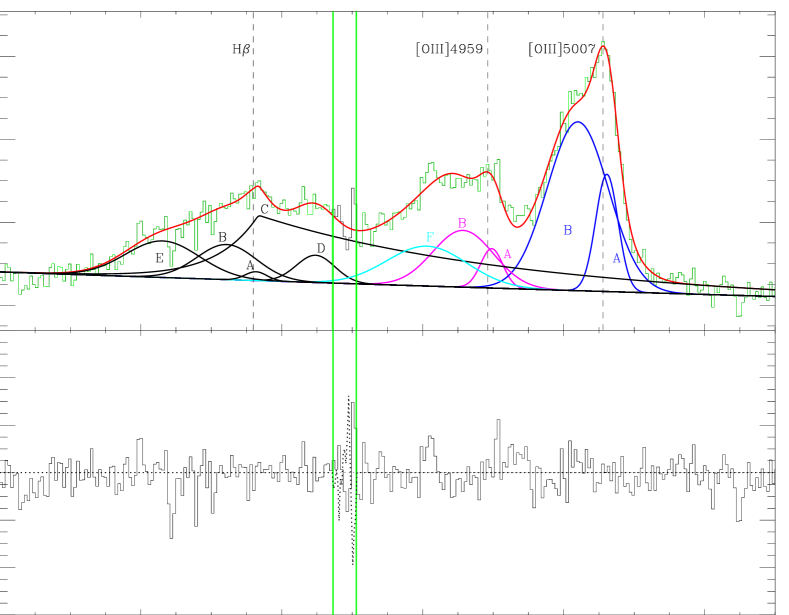
The H-band spectrum (Fig. 1) shows a clear broad H, associated with the broad line region (BLR), and a prominent [OIII] doublet, primarily associated with the quasar narrow line region (NLR). The [OIII]5007 line shows a clear asymmetric profile with a prominent blueshifted wing. This is generally a signature of outflows. Indeed, the lack of a corresponding redshifted wing is generally due to dust (in the host galaxy) absorbing the wind component on the opposite side of the galaxy disk, relative to our line of sight.
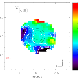
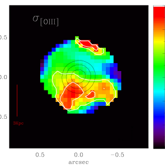
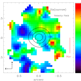
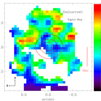
The [OIII] line is well fitted with two Gaussians as seen in Fig. 1. However, since the two [OIII] components are heavily blended, their fits are not independent. To avoid the possible ambiguities associated with the two components possibly being correlated, we investigate the [OIII] line kinematics by mapping the first and second moments of the global [OIII] profile (i.e. average velocity shift and dispersion). These two maps are shown in Fig. 2. Regions with S/N3 were masked out. As a zero velocity reference we have taken the peak of the [OIII] line in the central region (Fig. 1). The black contours indicate the location of the continuum. As shown by Fig. 2(left), the average velocity is strongly blueshifted with respect to the line peak, by a few hundred km/s, as a consequence of the strong blue asymmetry of the line. The velocity is strongly negative over the whole region where [OIII] is detected, suggesting that, if the prominent blue wing is due to a wind, then the outflowing ionized gas is distributed over all of the central 7 kpc. However, the most interesting features are the strongly blueshifted regions to the south and to the east of the nucleus, together making a bow-like morphology, suggestive of the envelope of a strong conical outflow. However, the observed velocity gradient may also be associated with rotation of the host galaxy disk (although the velocity field is certainly not a typical rotation curve). Outflow and galaxy rotation can be distinguished through the velocity dispersion: outflows are always associated with high velocity dispersion compared with regular motions in galaxy disks (e.g. Müller-Sánchez et al., 2011). The velocity dispersion map (Fig. 2) shows a large velocity dispersion over the whole region where [OIII] is clearly detected, suggesting that the whole central region is characterized by outflows. However, the velocity dispersion increases significantly in the SE region, where the strongly blueshifted gas is detected. This correspondence between blueshift and velocity dispersion strongly suggests that the blueshift observed in this region is due to an outflow excess and not to galaxy rotation.
While there is a general correspondence between velocity blueshift and dispersion, both with the highest values in the SE quadrant, a detailed analysis reveals interesting differences. The peak of the velocity dispersion is located between the two peaks of velocity blueshift. A possible interpretation is that those areas with highest velocity dispersion are associated with regions where the outflow is strongly interacting with the gas in the host galaxy disk, which also lowers the velocity locally.
The outflow may even be intrinsically symmetric, but the opposite (receding) outflow is likely to be obscured by dust in the host galaxy disk (as observed in local AGNs, Müller-Sánchez et al., 2011). It is interesting to note that the velocity dispersion map shows a strong excess in a tiny region on the NW (opposite to the main [OIII] outflow), this may be tracing the opposite outflow coming out of the galactic dusty disk.
The [OIII] line is primarily tracing gas in the NLR ionized by the QSO. Therefore, the most likely explanation is that the outflow is driven by the QSO radiation pressure. A quasar origin of the wind is also supported by the fact that the outflowing gas reaches velocities in excess of 1000 km/s (in the [OIII] blue wing), which cannot be explained by models of supernovae-driven outflows (Thacker et al., 2006). The mass of ionized outflowing gas is simply given by (see Appendix B)
| (1) |
where is the luminosity of the [OIII]5007 line tracing the outflow, in units of , is the electron density in the outflowing gas, in units of , typical of the NLR, and is the oxygen abundance is Solar units. If we assume that the outflow is traced by the broad component of [OIII], then , implying that the mass of ionized gas involved in the outflow is .
By assuming a simplified conical (or biconical) outflow distributed out to a radius (in units of kpc), then the outflow rate of ionized gas is given by (see Appendix B)
| (2) |
where is the outflow velocity in units of . The maximum outflow velocity inferred from the [OIII] profile is about 2000 km/s, which is probably representative of the average outflow velocity, while the lower velocities observed in the [OIII] line profile are very likely projection effects. By using , we infer an ionized gas outflow rate of about . This is a lower limit of the total outflow rate, since the ionized component is probably a minor fraction of the global outflowing gas mass. If we scale by the same neutral-to-ionized fraction as in Mrk231 (Rupke, priv. comm.), the total outflow rate can be up to an order of magnitude higher.
The inferred kinetic power of the ionized component of the outflow is about (Eq.11), or about times the bolometric luminosity of the AGNs (, from the continuum luminosity at 5100Å, and by assuming a bolometric correction factor of 7). However, if the ionized outflow is accompaneid by a neutral/molecular outflow an order of magnitude more massive, as discussed above, then the kinetic power is also likely to be an order of magnitude higher, i.e. about 1% of the bolometric luminosity, close to the expectation of quasar feedback models (Lapi et al., 2005).
3.2 H+[NII] analysis: evidence for quenched star formation
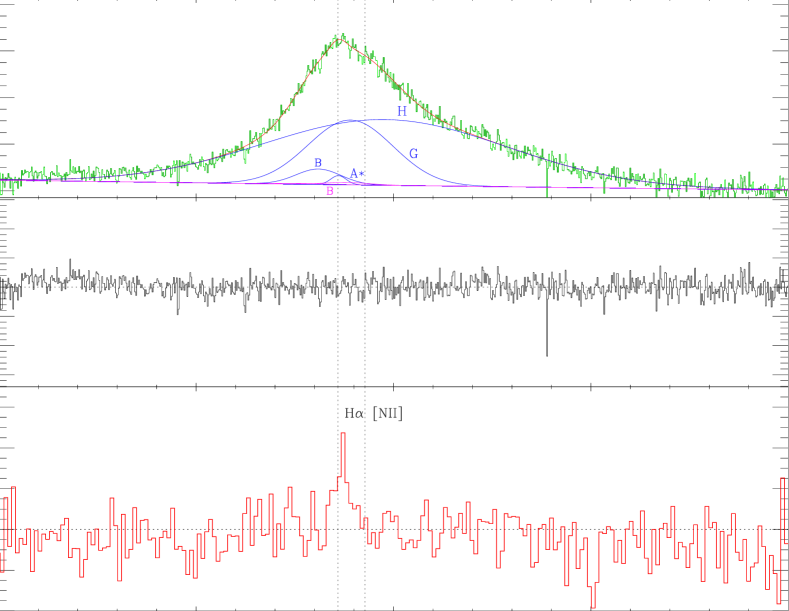
The has a very broad profile (from the BLR), and its overall profile has been fitted mostly with two broad Gaussians (see Appendix A for details). Interestingly, the fit also requires the presence of a weak, but significant narrow component of H (A*, FWHM). The absence of [NII] indicates that this narrow H emission is mostly due to star formation.
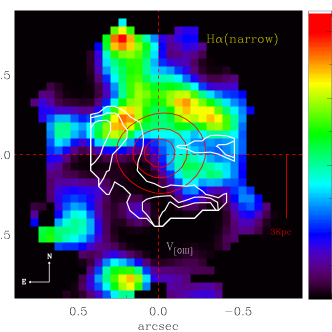
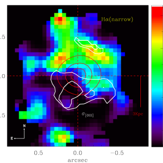
The map of the narrow H emission is shown in Fig.4, which reveals star formation extending over a few kpc from the nucleus. However, the star formation is not distributed symmetrically around the nucleus, but primarily towards the N and W. In particular, the region within a few kpc SE of the nucleus is nearly free of any narrow H tracing star formation. To show that the detection of narrow H and that the asymmetric distribution are not artifacts of the fitting procedure, we extracted a spectrum by integrating over the NW region putatively containing star formation, according to the H map, and another spectrum in the SE region devoid of star formation. After scaling the two spectra so that the intensity of the broad H wings (associated with the BLR) are the same, we have obtained the difference of the two spectra, which is shown in the bottom panel of Fig. 3. The differential spectrum clearly shows the presence of the narrow H. The line broadened profile (also making the detection noisier than expected ) is because we are integrating over different regions of the velocity field. The differential spectrum also confirms that no [NII] is detected in association with the narrow H, confirming that the latter is tracing star formation and not the quasar NLR.
We mention that the map of the [OIII] narrow component (shown in the appendix) is also characterized by a similar asymmetry towards the NE, suggesting that some of the [OIII] narrow line is associated with star formation. However, the asymmetry is less clean than observed for the H narrow component, likely because of NLR contribution to [OIII] and because of the blending with the “broad” [OIII] component.
The integrated emission of the narrow H yields a total star formation rate in the host galaxy of about (by using the conversion factor given in Kennicutt, 1998), which is not unusual in high-z quasars (e.g. Lutz et al., 2008). However, the most interesting result is that the star formation is heavily suppressed in the SE region, which is characterized by the excess of outflow with high-velocity dispersion. In Fig. 4(left) the white contours identify the strongest gas outflow traced by the highly blueshifted [OIII] line, as in Fig. 2-left, while in Fig. 4-right the white contours identify the highest velocity dispersion region, as in Fig. 2-right, which is likely the region where the strong outflow interacts with the host galaxy disk. We suggest that the heavy suppression of star formation in the region of strongest quasar-driven outflow among the first direct observational proofs of quasar feedback onto the host galaxy quenching star formation at high redshift, as predicted by models.
4 Conclusions
By using near-IR integral field spectroscopic observations we have revealed a powerful outflow in the host galaxy of the quasar 2QZ0028-28 at z=2.4. The outflow was revealed by the velocity field traced by the [OIII]5007 line, redshifted into the H-band. We estimated that the outflow rate of ionized gas is about , which is, however, a lower limit of the total gas outflow rate. Both the high outflow velocity () and the fact that the wind is mostly traced by the [OIII] line (produced primarily in the NLR) strongly suggest that the outflow is mostly driven by the quasar. The outflow is not symmetric, the highest velocities and highest velocity dispersion are found in the region SE of the nucleus.
In the K-band, our data clearly reveal the presence of narrow H emission tracing star formation in the host galaxy, on scales of several kpc and with a rate of about . However, star formation is not distributed uniformly in the host galaxy, but is mostly found in the regions not directly invested by the strong outflow. Instead, star formation is heavily suppressed in the SE region where the strongest outflow is detected. This observational result supports models invoking quasar feedback to quench star formation in massive galaxies at high redshift.
Acknowledgements.
We are grateful to the referee for his/her very useful comments. MCD is supported by the Marie Curie Initial Training Network ELIXIR under the contract PITN-GA-2008-214227 from the European Commission.References
- Alexander et al. (2010) Alexander, D. M., Swinbank, A. M., Smail, I., McDermid, R., & Nesvadba, N. P. H. 2010, MNRAS, 402, 2211
- Allen et al. (2011) Allen, J. T., Hewett, P. C., Maddox, N., Richards, G. T., & Belokurov, V. 2011, MNRAS, 410, 860
- Bower et al. (2006) Bower, R. G., Benson, A. J., Malbon, R., Helly, J. C., Frenk, C. S., Baugh, C. M., Cole, S., & Lacey, C. G. 2006, MNRAS, 370, 645
- Carilli & Wang (2006) Carilli, C. L., & Wang, R. 2006, AJ, 131, 2763
- Di Matteo et al. (2005) Di Matteo, T., Springel, V., & Hernquist, L. 2005, Nature, 433, 604
- Farrah et al. (2011) Farrah, D., Urrutia, T., Lacy, M., et al. 2011, arXiv:1112.1092
- Feruglio et al. (2010) Feruglio, C., Maiolino, R., Piconcelli, E., Menci, N., Aussel, H., Lamastra, A., & Fiore, F. 2010, A&A, 518, L155
- Fischer et al. (2010) Fischer, J., Sturm, E., González-Alfonso, E., et al. 2010, A&A, 518, L41
- Granato et al. (2004) Granato, G. L., Silva, L., de Zotti, G., Bressan, A., & Danese, L. 2004, Astrophysics and Space Science Library, 301, 129
- Hopkins et al. (2008) Hopkins, P. F., Cox, T. J., Kereš, D., & Hernquist, L. 2008, ApJS, 175, 390
- Kennicutt (1998) Kennicutt, R. C., Jr. 1998, ARA&A, 36, 189
- Lutz et al. (2008) Lutz, D., et al. 2008, ApJ, 684, 853
- King (2010) King, A. R. 2010, MNRAS, 402, 1516
- Lapi et al. (2005) Lapi, A., Cavaliere, A., & Menci, N. 2005, ApJ, 619, 60
- Maiolino et al. (2004) Maiolino, R., Oliva, E., Ghinassi, F., Pedani, M., Mannucci, F., Mujica, R., & Juarez, Y. 2004, A&A, 420, 889
- Menci et al. (2005) Menci, N., Fontana, A., Giallongo, E., & Salimbeni, S. 2005, ApJ, 632, 49
- Müller-Sánchez et al. (2011) Müller-Sánchez, F., Prieto, M. A., Hicks, E. K. S., et al. 2011, ApJ, 739, 69
- Nagao et al. (2006) Nagao, T., Marconi, A., & Maiolino, R. 2006, A&A, 447, 157
- Netzer et al. (2004) Netzer, H., Shemmer, O., Netzer, H., Maiolino, R., Oliva, E., Croom, S., Corbett, E., & di Fabrizio, L. 2004, ApJ, 614, 558
- Rupke & Veilleux (2011) Rupke, D. S. N., & Veilleux, S. 2011, ApJ, 729, L27
- Shemmer et al. (2004) Shemmer, O., Netzer, H., Maiolino, R., Oliva, E., Croom, S., Corbett, E., & di Fabrizio, L. 2004, ApJ, 614, 547
- Silk & Rees (1998) Silk, J., & Rees, M. J. 1998, A&A, 331, L1
- Sturm et al. (2011) Sturm, E., et al. 2011, ApJ, 733, L16
- Springel et al. (2005) Springel, V., Di Matteo, T., & Hernquist, L. 2005, MNRAS, 361, 776
- Thacker et al. (2006) Thacker, R. J., Scannapieco, E., & Couchman, H. M. P. 2006, ApJ, 653, 86
Appendix A Details of the spectral fitting
The initial spectral fit is performed on a spectrum extracted from a central aperture of ten pixels (i.e. 0.5 arcsec) in the H band and 20 pixels (i.e. 1.0 arcsec) in the K band, which guarantee high S/N.
The emission lines are fitted with multiple Gaussians and, in the case of the broad lines, by also using power-law profiles, as in Nagao et al. (2006). The continuum is fitted with a single power law, which represents the emission of the QSO accretion disk (plus possibly some minor contribution from the host galaxy stellar continuum). Starting from this initial fit in the central region, we fitted the spectra individually at all spatial pixels by leaving most of the parameters free, except for the velocity, dispersion, and relative intensity of the components describing the broad lines (H and H). Indeed, since the BLR is unresolved, the shape and shift of the broad line profile (components C+D+E in the case of H) must be constant over the field of view, and there the global intensity variation only reflects the seeing PSF. We tried to also include an Fe II template in the spectral fitting (as in Netzer et al., 2004); however, this is always set to zero by the fitting procedure, confirming the lack of significant FeII emission inferred by the visual inspection of the spectrum. This result contrasts with the measurement of Netzer et al. (2004), who obtain a flux of the Fe II emission that is about 0.37 times the H emission, and we ascribe the discrepancy to the much lower signal-to-noise in the latter spectrum.
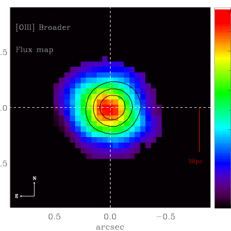
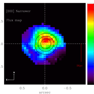
Figure 1 shows the various components used to fit the H-band spectrum of the central region and, in the bottom panel, the fit residuals. The region included within the two green lines is affected by strong sky residuals and was not considered in the fit. In this figure we can see that the [OIII] profile can be nicely fitted with two Gaussians, one relatively narrow (A, FWHM600 km/s) and a second one (B) blueshifted by about 700 km/s and with FWHM1700 km/s (much broader than typically found in the NLR of lower luminosity AGNs). The [OIII]4959 line is fitted with the same components, linked to have an intensity equal to one third of the [OIII]5007 line. Figure 5 shows the flux distribution of the broad and narrow components of [OIII]. The peak of the [OIII] broad component is shifted towards the SE, i.e. in the same direction as the strong outflow, confirming that this is the region where the NLR develops and where the quasar radiation pressure is driving the outflow. The narrow component of [OIII] is instead distributed towards the N and towards the W, i.e. similar to the H narrow component, suggesting that the narrow component of [OIII] receives a significant contribution from star formation. However, the imperfect correspondence between the two maps suggests that a fraction of the narrow [OIII] is also contributed by the NLR.
The [OIII]4959 line is heavily blended with another line at , which is also seen in the spectra of other quasars, sometimes tentatively identified with FeII emission; however, in the quasar discussed here (as well as in a few others showing the same feature), the iron emission that typically encompasses the H+[OIII] group is particularly weak, therefore suggesting a different origin of this line. In the residuals we observe a narrow component that is likely associated to the same unidentified line. The fit of the broad H requires three Gaussians and a powerlaw profile (as in Nagao et al. 2006). We also included the H contribution associated with the two [OIII] components. However, one should bear in mind that the intensity of these weaker H components is difficult to evaluate, since these are blended within the broad, complex H profile. In Table 1 we list the parameters inferred for all of the components used in the fitting of the SINFONI spectra.
The H profile (dominated by the broad component, tracing the BLR) is clearly different from the H profile, which is a property that is common to many other quasars and AGNs and that is ascribed to complex radiative transfer within the dense gas of the BLR. The bulk of the H profile was fitted by using two very broad Gaussians (H and G in Fig. 3), which give the seeing in the K-band, which is roughly consistent with the seeing measured in the H-band observation. As for the broad H, the relative intensity, shift, and width of these two lines are kept fixed over the field of view, and their overall intensity variation reflects the seeing PSF.
We forced the inclusion of component B in the H profile, by using the same velocity shift and width as the corresponding [OIII] component, while the intensity was left free to vary. This component of H is certainly associated with the NLR. However, since this component is relatively broad, its intensity is poorly constrained (see uncertainty in the flux of this component in Table 1), and degenerate with the other two broad H Gaussian components (as is the case for the corresponding component in H). The [NII] doublet associated with component B is also forced to have the same shift and width as the corresponding [OIII] component. The relative intensity of the two [NII]6548,6584 lines are forced to be in the ratio of 1:3. The intensity of these [NII] lines is even less constrained than the corresponding H B component, since the wavelength of [NII]6548 nearly overlaps the intense component G of H. The resulting [NII]/H ratio of component B is low, but highly uncertain (), but still consistent with the values observed in AGNs.
The narrow component “A” is much narrower than the other components and, therefore, easier to disentangle from the broad H profile. However, in principle, we should include two narrow () H components, one associated with the quasar NLR and another one associated with any putative star formation in the host galaxy. However, the quality of our data does not really allow us to fit two separate narrow components, because these would be totally degenerate. We therefore fit a single narrow component not tied to have the same velocity and width of component “A” of [OIII]. We label this narrow H component with “A*” (meaning that it may be partly associated with component A of [OIII], but not necessarily). We investigate the relation of the H component “A*” with the [OIII] component “A” a posteriori. We note that it is not possible to follow a similar approach on H (i.e. introduce a component “A*”, not linked to the [OIII] components, since, besides the problem of the blending with other components, the signal-to-noise on H is much lower).
The parameters resulting from the best fit in the K-band are given in Table 1. We note that there is no room for narrow A* [NII] emission, at a level of . The lack of an [NII] narrow component is confirmed by the “differential” spectrum presented in Sect. 3.2 and in Fig. 3, which is totally independent of any fitting procedure. As discussed in the body of the paper, the lack of [NII] at a level below one fourth of H indicates that this narrow H emission is mostly tracing star formation, and not the NLR.
Figure 6 shows the velocity field and the velocity dispersion of the narrow component of H. Both maps are very noisy, owing to the weakness of the line. The velocity field does not clearly indicate a rotation pattern, which would be expected by gas in a galactic disk, except possibly for an NW-SE gradient, but the latter may be associated with some contribution to H narrow from the outflow in the SE region. However, only a fraction of the disk is actually traced by the H narrow, and this, together with the noisy velocity map, may prevent identification of a clear rotation pattern. Moreover, it is well known that host galaxy disks of optically selected quasars tend to be face on, as a consequence of selection effects (Carilli & Wang, 2006), so it is not expected that quasar host galaxies have prominent rotational patterns. The velocity dispersion map is very noisy, but it is consistent with being uniform over the area where H narrow is detected.
We finally note that the best-fit velocity and FWHM of component A* of H are similar to component A of [OIII]. This further suggests that the latter component of [OIII] is partly contributed by the ionized gas in the star-forming regions traced by the narrow H. The inferred , at the verge of the range typically observed in star-forming galaxies, indicates that the flux of component A of [OIII] is not incompatible with being partly originated by star formation, but probably a contribution by the AGN NLR is required. As mentioned above, the similarity of the map and the map also supports the scenario where part of component A of [OIII] is associated with star formation.
| Line | Component | Fitting Function | FWHM | Flux | Velocity1 | |
| (m) | (km/s) | () | (km/s) | |||
| [OIII]5007 | A | Gaussian | 1.7061 | 652 | 10.90.56 | 92 |
| B | Gaussian | 1.7020 | 1797 | 43.62.3 | -663 | |
| H | A | Gaussian | 1.6564 | 652 | 0.790.66 | 92 |
| B | Gaussian | 1.6522 | 1797 | 8.83.6 | -663 | |
| C | Broken Power Law | 1.6567 | 5508 | 57.94.6 | 156 | |
| D | Gaussian | 1.6648 | 1150 | 4.42.9 | 1622 | |
| E | Gaussian | 1.6431 | 2243 | 11.30.26 | -2306.6 | |
| No ID | F | Gaussian | 1.6806 | 2378 | 13.182.3 | — |
| H | A* | Gaussian | 2.2361 | 616 | 1.90.3 | 20 |
| B | Gaussian | 2.2310 | 1797 | 9.33.5 | -663 | |
| G | Gaussian | 2.2391 | 3386 | 73.75.5 | 422 | |
| H | Gaussian | 2.2478 | 9717 | 220.810.4 | 1588 | |
| [NII]6584 | A* | Gaussian | 2.24331 | 6161 | 0.4 | 72 |
| B | Gaussian | 2.2382 | 1797 | 1.71.5 | -663 |
The names of the components correspond to those shown in Figs. 1 and 3. Notes: 1 The velocities of the components are obtained by assuming the peak of [OIII]5007 as a rest frame reference. 2 For this [NII] line, the width and velocity were forced, to estimate the upper limit to the values found for the corresponding A* component in H.
Appendix B A simple model of the ionized outflow
In this section we discuss how the physical properties of the ionized outflow can be constrained through the observational parameters of the [OIII] line, by adopting a simple model for the ionized wind. The [OIII]5007 line luminosity associated with the outflow is simply given by
| (3) |
where is the volume occupied by the outflowing ionized gas, the filling factor of the [OIII] emitting clouds in the outflow, and the [OIII]5007 emissivity that, at the temperature typical of the NLR (), has a weak dependence on the temperature (). It can be expressed by
| (4) |
where is the energy of the [OIII]5007 photons (in units of ), and are the volume densities of the ions and of electrons, respectively (in units of ). Under the reasonable assumption that most of the oxygen in the ionized outflow is in the form, then
| (5) |
where gives the oxygen abundance in solar units.
The mass of outflowing ionized gas is given by
| (6) |
where is the mass of the hydrogen atom, and where we have neglected the mass contributed by species heavier than helium.
By combining Eqs. 3 and 6 we obtain
| (7) |
where is the luminosity of the [OIII]5007 line emitted by the outflow, in units of , () is the average electron density in the ionized gas clouds, in units of , and is a “condensation factor”, where . We can assume under the simplifying hypothesis that all ionizing gas clouds have the same density. Also, under these assumptions, the mass of outflowing ionized gas is independent of the filling factor of the emitting clouds.
If we assume a simplified model of the outflow (justified by the limited information currently available to us) where the wind occurs in a conical region, with opening angle , composed of ionized clouds uniformly distributed and outflowing with velocity , out to a radius , then the mass outflow rate of ionized gas is given by
| (8) |
where is the average mass density in the whole volume occupied by the outflow, which is given by
| (9) |
where the volume occupied by the conical outflow is given by . Unless , generally , since the latter numerical density (defined above) is averaged among the emitting clouds, not over the whole volume.
By replacing Eqs. 7 and 9 into Eq. 8 we obtain that the ionized outflow rate is given by
| (10) |
where , , and () were defined above, is the outflow velocity in units of , and is the radius of the outflowing region, in units of kpc. The outflow rate is independent of both the opening angle of the outflow and of the filling factor of the emitting clouds (under the assumption of clouds with the same density).
The kinetic power (associated with the ionized component) is then given by
| (11) |