P/2010 A2 LINEAR

Comet P/2010~A2 LINEAR is an object on an asteroidal orbit within the inner Main Belt, therefore a good candidate for membership with the Main Belt Comet family. It was observed with several telescopes (ESO New Technology Telescope, La Silla, Chile; Gemini North, Mauna Kea, Hawai‘i; University of Hawai‘i 2.2 m, Mauna Kea, Hawai‘i) from 14 Jan. until 19 Feb. 2010 in order to characterize and monitor it and its very unusual dust tail, which appears almost fully detached from the nucleus; the head of the tail includes two narrow arcs forming a cross. No evolution was observed during the span of the observations. Observations obtained during the Earth orbital plane crossing allowed an examination of the out-of-plane 3D structure of the tail. The immediate surroundings of the nucleus were found dust-free, which allowed an estimate of the nucleus radius of 80–90 m, assuming an albedo $p=0.11$ and a phase correction with $G=0.15$ (values typical for S-type asteroids). A model of the thermal evolution indicates that such a small nucleus could not maintain any ice content for more than a few million years on its current orbit, ruling out ice sublimation dust ejection mechanism. Rotational spin-up and electrostatic dust levitations were also rejected, leaving an impact with a smaller body as the favoured hypothesis. This is further supported by the analysis of the tail structure. Finston-Probstein dynamical dust modelling indicates the tail was produced by a single burst of dust emission. More advanced models (described in detail in a companion paper), independently indicate that this burst populated a hollow cone with a half-opening angle $\alpha\sim 40\degr$ and with an ejection velocity $v_{\rm max}\sim 0.2$ m s^-1, where the small dust grains fill the observed tail, while the arcs are foreshortened sections of the burst cone. The dust grains in the tail are measured to have radii between $a=1$–20 mm, with a differential size distribution proportional to $a^{-3.44\pm 0.08}$. The dust contained in the tail is estimated to at least $8\times 10^{8}$ kg, which would form a sphere of 40 m radius (with a density $\rho=3\,000$ kg m^-3 and an albedo $p=0.11$ typical of S-type asteroids). Analysing these results in the framework of crater physics, we conclude that a gravity-controlled crater would have grown up to $\sim 100$ m radius, i.e. comparable to the size of the body. The non-disruption of the body suggest this was an oblique impact.

1 Introduction

Habitability within our solar system is determined by the distribution of water and volatiles, yet the origin of this distribution is currently a fundamental unresolved planetary science issue (Kasting & Catling 2003). There are three leading scenarios for the origin of terrestrial planetary water, including: ($i$) nebular gas adsorption on micron-sized dust grains inside the snow line (Muralidharan et al. 2008, the distance from the Sun outside of which water the temperature is low enough for water ice to condense), ($ii$) chemical reactions between an early hydrogen envelope and oxides in a magma ocean Genda & Ikoma (2007, 2008), or ($iii$) delivery by volatile-rich planetesimals (asteroids or comets) formed beyond the snow line (Morbidelli et al. 2000). The first two processes probably contributed to, but may be unable to account for all of Earth’s water (Mottl et al. 2007). Within the broader context of icy bodies, main belt comets (MBCs), a newly discovered class of “comets having stable orbits completely confined to the main asteroid belt” (Hsieh & Jewitt 2006), present a subclass of particular significance to the history of terrestrial water and other important volatiles.

In addition to possibly P/2010 A2 (LINEAR), there are currently five known MBCs: 133P/Elst-Pizarro, 176P/LINEAR, 238P/Read, C/2008 R1 (Garradd) and P/2010 R2 (La Sagra). The main belt comets are defined (Hsieh & Jewitt 2006) by ($i$) a semi-major axis that is less than Jupiter’s, ($ii$) Tisserand parameters significantly greater than 3 —meaning they are dynamically decoupled from Jupiter, like ordinary asteroids (Vaghi 1973; Kresak 1980)— and ($iii$) mass loss with a cometary appearance. As comets in near-circular orbits within the asteroid belt, these objects likely still harbor nebular water frozen out from beyond the primordial “snow line” (Encrenaz 2008; Garaud & Lin 2007) of the young solar system. Dynamical simulations suggest they probably formed in-situ (Haghighipour 2009) at a different temperature from either comets or the asteroidal reservoir that has been sampled through our meteorite collections. Thus, understanding their chemistry can provide unique insight into the distribution of volatiles in the early stages of planet formation.

P/2010 A2 (LINEAR) was discovered by the LINEAR project on 7 Jan., 2010 (Birtwhistle et al. 2010a) and was described as “a headless comet with a straight tail, and no central condensation” (Birtwhistle et al. 2010b). On 11–12 Jan., observers at the WYNN 3.5-m and at the 2.5-m Nordic Optical Telescope reported that the object had a asteroidal-like body $\sim$ 150–200m in diameter which was connected to the tail by an unresolved light bridge (Green 2010). Based on the orbital semi-major axis and on the Tisserand parameter, $T_{J}=3.6$, Jewitt (Green 2010) concluded that P/2010 A2 was a new MBC. With the smallest perihelion distance of any of the MBCs ($q=2.29$ AU), these elements suggested a membership in the Flora family. Flora is a large asteroid family of $\sim$500 members which can be broken up into many sub-families or clans and which are broadly compositionally consistent with space-weathered S-type asteroidal spectra (Florczak et al. 1998). Jewitt (Green 2010) and Licandro (Haver et al. 2010) suggested that the location of the nucleus outside the coma might be the consequence of an impact.

Is P/2010 A2 a genuine, sublimating comet (whose activity was possibly triggered by an impact), or is the tail the signature of an impact (or another alternative process), with a dispersion of the dust ejecta but no sublimation? If it can be demonstrated that the object is a comet, it would indicate that at least one object in the inner asteroid belt still contains volatile material. The water snow line in the proto-solar nebula is estimated to have been around 2.5 AU from the Sun (Jones et al. 1990) or possibly even as close as 1.5 AU (Lecar et al. 2006; Machida & Abe 2010; Min et al. 2011). Initially parent bodies beyond the snow line are believed to be mixtures of water ice and silicates, which are then heated due to the radioactive decay of ²⁶Al within 1–2 million years after nebular collapse (Krot et al. 2006). Grimm & McSween (1989) find that once the water is liquid, it is consumed by hydration reactions, preferentially in the interior (Cohen & Coker 2000; Wilson et al. 1999), possibly leaving ice in the outer layers. In the inner asteroid belt, it is likely that most of that water has been converted in hydrated material observed on S-type asteroids (Rivkin et al. 2002). MBCs may be the frozen components of the outer edges of asteroid parent bodies that have survived the age of the solar system.

Four of the MBCs are located in the outer main belt, where asteroids with hydrated material are less common, suggesting water ice could still exist. The orbital elements of the MBCs are listed in Table 1 and displayed in Fig. 1. 133P/Elst-Pizarro, the first MBC discovered, is a member of the Themis family; 176P/LINEAR was found in a survey targeting objects with orbits similar to that of 133P/Elst-Pizarro (Hsieh 2009). 238P/Read, however, was discovered serendipitously (i.e. not within a MBC-dedicated program) on a similar orbit. A fourth MBC, P/2008 R1 Garradd, was discovered serendipitously in the central region of the main belt. The fifth MBC, P/2010 R2 La Sagra, was also discovered serendipitously with a semi-major axis similar to that of 133P/Elst-Pizarro (Marsden et al. 2010). More recently, asteroid (596) Scheila presented a comet-like appearance (Larson 2010). Bodewits et al. (2011) and Jewitt et al. (2011) conclude however that this dust cloud was likely caused by the impact of a small asteroid on Scheila. The survival of an icy body in the inner asteroid belt would therefore give exciting constraints on the evolution of water in the belt. It would also raise fundamental questions on how to shield water ice in that area of the solar system in a rather small body.

Figure 1: (not available on astroPh) The orbital elements of P/2010 A2 (green square to the left), of the 5 known MBCs (circles, 133P and 238P are indistinguishable) and of the numbered main belt asteroids (small dots). When available, the proper elements were used (source: the Asteroid Dynamics Site, http://hamilton.dm.unipi.it/astdys/). The inclination of P/2010 R2 La Sagra is off scale; its $a$ is marked by a triangle on the top of the plot; $i=21.39$ .

a.
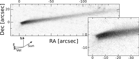
b.
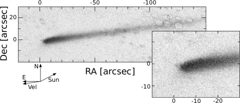
c.
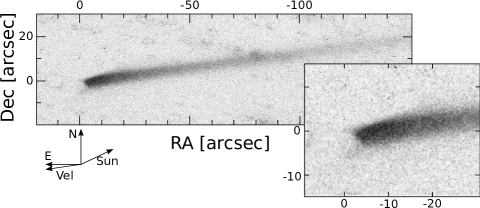
d.
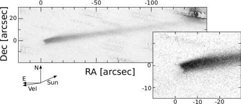
e.

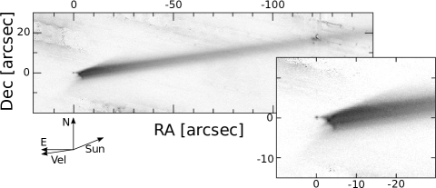
Figure 2: P/2010 A2, images from UT 14.2 (a), 16.2 (b), 17.2 (c), 18.2 (d) Jan. 2010 using the NTT, UT 19.5 Jan. 2010 using GN (e). The linear gray scale covers the range of (0–3) $\times 10^{-8}Af$, a proxy for the amount of dust present (see Section 3.3.3). Each panel includes a 40$\times 30^{\prime\prime}$ zoomed portion to show details of the inner structure. The positions of N and E are indicated, as are the anti-solar direction and the heliocentric velocity vector.

f.
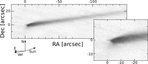
g.
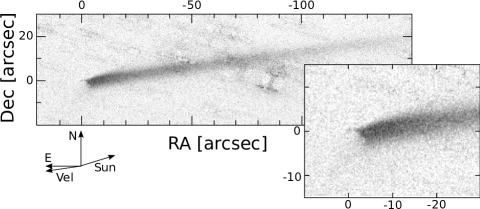
h.
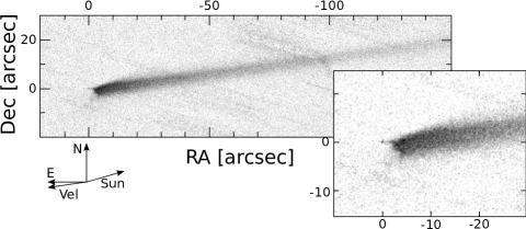
i.
j.

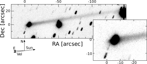
Figure 2: continued. P/2010 A2, images from UT 22.3 (f), 23.4 (g), 25.4 (h) Jan. 2010 using UH 2.2-m, UT 2.3 Feb. 2010 using GN (i), UT 19.5 Feb. 2010 using UH 2.2-m (j).

Moreno et al. (2010) presented observations obtained with the GTC, WHT and NOT on La Palma, which they modeled with an extended period of water-driven cometary activity. Jewitt et al. (2010) acquired a series of HST images; from the orientation and geometry of the tail, they favor the disruption of an asteroid (either by collision or spin up) in Feb.–Mar. 2009. Finally, Snodgrass et al. (2010) secured observation from the Rosetta spacecraft. Thanks to the position of the space probe, they could observe the object with a very different geometry (but with a much more modest resolution), from which they concluded that the observed dust tail was caused by an impact.

In order to investigate the process that generated the observed dust tail, we acquired deep images of P/2010 A2 over various epochs. The observations are presented in Section 2. The analysis and modelling of the nucleus and dust are described in Section 3. In Section 4, we discuss the conclusions and summarize the results. A companion paper (Kleyna et al. 2011) is devoted to the details of the dust models developed for this study, and a second follow-up article (Hermalyn et al. 2011) focuses on the characteristics of the impact process and of the nucleus based on the interpretation of the dust as an impact plume.

2 Observations

The telescopes and instruments used are described below. The epoch, geometric circumstances and a log of the observations are listed in Table 2.

In all cases, the observations were acquired as series of fairly short individual exposures obtained while tracking at the non-sidereal motion rates of the comet, and offsetting the telescope position between exposures.

2.1 Telescopes and Instruments

2.1.1 New Technology Telescope

The observations were performed on the ESO 3.56m New Technology Telescope (NTT) on La Silla, with the ESO Faint Object Spectrograph and Camera (v.2) instrument (EFOSC2) (Buzzoni et al. 1984; Snodgrass et al. 2008), through Bessel $B$, $V$, $R$, and Gunn $i$ filters, using the ESO#40 detector, a 2k$\times$2k thinned, UV-flooded Loral/Lesser CCD, which was read in a 2$\times$2 bin mode resulting in $0\aas@@fstack{\prime\prime}24$ pixels, and a $4\aas@@fstack{\prime}1$ field of view.

2.1.2 Gemini North Telescope

The observations were acquired in queue-mode on the 8.1-m Gemini North (GN) Telescope on Mauna-Kea, using Gemini Multi-Object Spectrograph (GMOS) (Hook et al. 2004), through a SDSS $r^{\prime}$ filter (Fukugita et al. 1996). The detector mosaic is composed of three 2k$\times$4k EEV CCDs arranged in a row, resulting in an un-vignetted field of view of $5^{\prime}$. The detectors were binned $2\times 2$ resulting in a $0\aas@@fstack{\prime\prime}145$ projected pixel size.

2.1.3 Univertity of Hawai‘i

The observations were performed on the University of Hawai‘i (UH) 2.2-m telescope on Mauna-Kea, using the Tektronix 2k$\times$2k CCD camera (Wainscoat 2010). The projected pixel size is $0\aas@@fstack{\prime\prime}22$, and the field of view $7\aas@@fstack{\prime}5$. Kron-Cousin $B$, $V$, $R$, $I$ and SDSS $r^{\prime}$ filters were used.

Table 1: Elements of P/2010 A2 and the five known MBCs

Object	$a$ [AU]	$e$	$i$	$T_{J}$
176P/(118401) LINEAR	3.217	0.150	1.352	3.172
133P/(7968) Elst-Pizarro	3.164	0.154	1.370	3.185
238P/Read (P/2005 U1)	3.165	0.253	1.266	3.153
P/2008 R1 Garradd	2.726	0.342	15.903	3.216
P/2010 R2 La Sagra	3.099	0.154	21.394	3.203
P/2010A2 LINEAR	2.291	0.124	5.255	3.588

Table 2: Observation Log

Obs. date	$r^{1}$	$\Delta^{2}$	$\alpha^{3}$	PsAng4	PsAMV5	PlAng6	Tel-Ins7	Who8	Obs.9		Seeing	Comments
UT 2010	[AU]	[AU]	[deg]	[deg]	[deg]	[deg]					[arcsec]
14.2 Jan.	2.013	1.040	5.6	123.3	280.1	-2.2	NTT	OH	1200	B,	1.6	Poor seeing
							EFOSC2		600	V,
									2400	R,
									800	i
16.2 Jan.	2.014	1.045	6.7	117.7	279.8	-2.0	NTT	HH	900	B,	1.4	Poor seeing
							EFOSC2		600	V
									1500	R,
									600	i
17.2 Jan.	2.014	1.048	7.2	115.5	279.7	-2.0	NTT	HH	600	B,	1.1
							EFOSC2		600	V
									1200	R,
									600	i
18.2 Jan.	2.015	1.051	7.8	113.6	279.6	-1.9	NTT EFOSC2	HH	3600	R	0.9–1.6
19.5 Jan.	2.015	1.055	8.5	111.5	279.4	-1.8	GN GMOS	OH/GT	3000	r′	0.5–0.7	Excellent seeing.
22.3 Jan.	2.016	1.066	10.0	107.9	279.1	-1.5	UH Tek	BY	1800	B	0.5-0.8
							Tek		1750	V
									7250	R,
									1800	I
23.4 Jan.	2.017	1.071	10.6	106.8	279.0	-1.4	UH Tek	BY	3000	R	1.0
25.3 Jan.	2.018	1.080	11.7	105.2	278.8	-1.3	UH Tek	BY	4000	r′	0.7
02.3 Feb.	2.022	1.125	15.6	100.4	278.3	-0.6	GN GMOS	OH/GT	3000	r′	0.5
19.5 Feb.	2.032	1.262	22.3	96.3	278.3	0.7	UH Tek	JP	1500	R	1.2	Star on object

Notes: 1, 2: Helio- and geocentric distances; 3: Solar phase angle; 4: Position angle of the extended Sun-Target radius vector; 5: Position angle of the negative of the target’s heliocentric velocity vector; 6: Angle between observer and target orbital plane, measured from target; 7: Telescope and instrument: NTT= New Technology Telescope, GN= Genini North, UH= UH 2.2-m; 8: Observer initials: OH= O. Hainaut, HH= H. Hsieh, GT= G. Trancho, BY= B. Yang, JP= J. Pittichová 9: Total on-target exposure time [sec], and filter.

2.2 Data Processing

The images were corrected for instrumental signature by subtracting a master bias frame and dividing by a master flat-field frame obtained from twilight sky images. Because of the large angular size of the object, we have not applied second order, “super-flatfield” technique. In the case of the Gemini images, the basic processing was performed using the GMOS tasks from the Gemini IRAF Package (version 1.9) , which also corrects for the geometric distortion and merges the three chips into single images. The frames were flux calibrated using nightly images of Landolt (1992) fields obtained over a range of airmasses.

In order to create deep composite images to assess the extent of the dust, offsets between images were measured and corrected for using series of field stars. The motion of the comet was then compensated for using either the linear ephemeris rates, or a full astrometric solution to compute the offset between expected positions of the comet from JPL’s Horizon ephemerides. The frames were shifted and then combined using either a median combination or an average rejecting the pixels deviating the median value, in order to remove the stars and background objects as well as detector defects and cosmic ray hits. In some cases, individual stars were masked and rejected during the combination. The resulting $R$-band (or equivalent) images for each run are presented in Fig. 2. A zoomed portion of the head of the object is included in each panel in order to show the details of the inner structure.

3 Analysis

3.1 Description

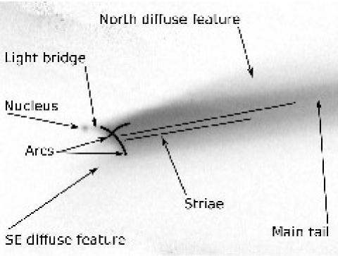
Figure 3: Schematic of the main features of P/2010 A2. The background image is the 19 Jan. GN image from Fig. 2.e. See also Fig. 4 for enhancement of the features.

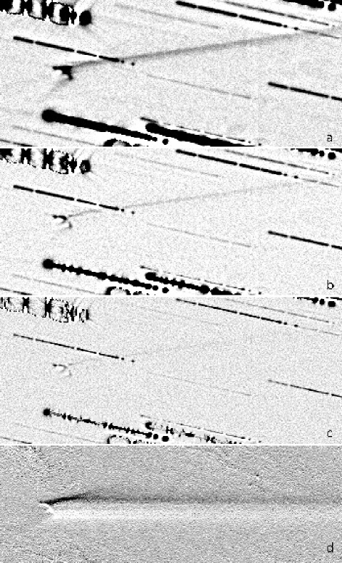
Figure 4: UT 19 Jan. 2010 GN image of P/2010 A2 (Fig. 2.2), enhanced using unsharp masking, with a window of 20 (a), 10 (b) and 5 pixel radius (c). Panel (d) was produced by shifting the image by 1 pixel vertically and subtracting the result from the original, after rotating the image to align the tail along the rows.

Following the nomenclature introduced by Jewitt et al. (2010) in their Fig. 1 describing their Hubble observations, the main features of the comet are a principal nucleus connected via a very faint and narrow light bridge to an arc-shaped dust feature (see Fig. 3). A second arc-shaped feature crosses the first one almost perpendicularly. The main tail extends from these two arcs. Very narrow striae along the main tail are emanating from knots in the arcs. A low surface brightness fin-shaped structure lies above (North) of the main tail. A second low surface brightness more diffuse structure (not reported on the Hubble images) extends to the SE of the arcs.

A variety of unsharp masking techniques were used to enhance the tail structures. A filter consisting of a sliding circular window of radius $n$ pixels was moved through the 19 Jan. GN composite image and the central pixel in the window was replaced by the median of the pixels in the window. The resulting smoothed image was subtracted from the original image to remove the background thus enhance the high frequency components. The results for windows of 20, 10 and 5 pixel radii are shown in Fig. 4. The 20 pixel radius filtering window brings out a broad dust feature at PA $\sim 310\degr$, the “North fin”, which is roughly in the anti-solar direction. The dust modelling described below gives some hints on the origin of that features, which are discussed in Section 3.3.6. Additionally, the shifted individual GN images were median combined, and rotated by 8.3^∘ to place the tail along a row.

The rotated image was then shifted by 1 pixel vertically and subtracted from the composite to enhance structures along the dust tail. This is also shown in Fig. 4, panel [d]. Each of the condensations of material in the arc are shown to be secondary sources of dust.

The available data-set covers a period of 36 days, during which the Earth crossed the object orbital plane (from -2.2$\degr$ to 0.6$\degr$). The morphology of the comet is remarkably constant over that time, implying that the motion of the dust is slow, and that the observed dust features have a significant thickness above the orbital plane. This, in turn, implies the dust was ejected with a non-zero velocity. We searched for evolution in the morphology between the various epochs of observation, but given the observation interval and resolution of the ground-based images, no changes in structure were observed.

3.2 The nucleus

3.2.1 Measurements

The nucleus brightness was measured on the two GN datasets, through a series of apertures of increasing radius. The best compromise between enclosed signal and sky background noise is found for an $0\aas@@fstack{\prime\prime}3$ radius aperture. The nucleus magnitude measured in that aperture is corrected for the missing flux using the star growth profile as a reference. The resulting magnitudes are listed in Table 3.

Table 3: Nucleus photometry

UT (exposure start)		Exp.time	Airmass	Filter	Seeing	Mag	M(1,1,$\alpha$)	M(1,1,0)
		[s]			[′′]	$r$’	$r$’	$r$’
2010-01-19	11:27:03.3	600.	1.16	r	0.58	23.93$\pm$0.04
2010-01-19	11:37:51.3	600.	1.19	r	0.60	23.77$\pm$0.03
2010-01-19	11:48:38.2	600.	1.22	r	0.63	23.96$\pm$0.04
2010-01-19	11:59:25.2	600.	1.26	r	0.70	24.01$\pm$0.03
2010-01-19	12:10:12.1	600.	1.30	r	0.81	24.20$\pm$0.04
2010-01-19	average			r			22.34$\pm$0.04	21.74$\pm$0.04
2010-02-02	06:32:55.1	600.	1.09	r	0.93	*
2010-02-02	06:43:42.9	600.	1.08	r	0.93	*
2010-02-02	06:54:30.9	600.	1.06	r	0.78	24.03$\pm$0.08
2010-02-02	07:05:17.8	600.	1.05	r	0.92	24.38$\pm$0.06
2010-02-02	07:16:04.8	600.	1.03	r	0.75	24.00$\pm$0.06
2010-02-02	average			r			22.35$\pm$0.05	21.55$\pm$0.05

Note: *= the nucleus was contaminated by a field star.

The radial profile of the nucleus was measured between PA $-40$ and 110$\degr$ (i.e. the area not affected by the tail). This was done by converting the $(x,y)$ of each pixel to an angle and a distance, then the flux is averaged between the two position angles for each distance range. The surface brightness profiles are then constructed by iteratively adjusting the asymptotic level of the brightness profile so that it reaches zero. The error bars shown in Fig. 5 therefore reflect a robust estimate of the sky noise. The average profile is compared to that of a field star (measured perpendicularly to the trailing). The profiles corresponding to the image with the best seeing are displayed, normalized to the same peak brightness, in Fig. 5. The P/2010 A2 profile shows no significant excess for radii smaller than 3 pixels ($0\aas@@fstack{\prime\prime}42$), then a (noise) extended contribution barely above the sky level.

In order to obtain a conservative estimate of the quantity of dust directly surrounding the nucleus, the upper limit on flux excess from the nucleus profile with respect to the reference star was integrated out to a radius of $2^{\prime\prime}$. The upper limit on the flux excess in an annulus is defined as the measured surface brightness of the comet minus that of the comparison star, plus a 1-$\sigma$ error bar, multiplied by the area of the annulus. The limit on the flux excess integrated to a radius of $2^{\prime\prime}$ corresponds to a mag $27.7$, or $<3$% of the flux from the nucleus. The nucleus did not present any significant mass-loss at the time of the observations. This is further confirmed by the lack of any dust visible in the lower-left (SE) quadrant below the nucleus, as discussed in Section 3.3.2. This strengthens the conclusion of Jewitt et al. (2010) that there was no cometary activity based on the purely geometric variation of nucleus brightness with heliocentric distances, withing 0.6 mag, from 25 Jan. until 29 May. 2010.

The average measured $r^{\prime}$ magnitudes convert to absolute magnitudes $r^{\prime}(1,1,\alpha)=22.34\pm 0.04$ and $22.35\pm 0.05$ for the two GN runs. We do not have enough data to estimate the solar phase effect. We therefore use the typical S-type asteroid $G=0.15$ to correct for this effect, assuming the object is either a member of the Flora family, or of the most frequent type in that region of the solar system. The phase-corrected absolute magnitudes are $r^{\prime}(1,1,0)=21.74\pm 0.04$ and $21.55\pm 0.05$. The uncertainty is however now dominated by the uncertainty of the phase correction, which could be off by 0.08 mag if the object is asteroidal but not of the S-type (Jedicke et al. 2002), and by 0.10–0.15 if the object is a low albedo comet. The magnitude difference between the two epoch is likely to dominated by the rotational variability; indeed a body this small is likely to have lightcurve amplitude of many tenth of magnitude.

Using the colour equations for the SDSS filters from Fukugita et al. (1996), the solar magnitude in the Sloan filter is $r^{\prime}_{\sun}=-26.95$ (Ivezić et al. 2001). Assuming a typical S-type asteroid albedo of $p=0.11$, the absolute magnitude corresponds then to a radius of 80 and 90 m for the two epochs. The formal uncertainty on this value is completely dominated by the assumption of the albedo and phase correction, and certainly includes a variation caused by the rotation of the nucleus. This is in agreement with the radius of 58–77 m reported by Jewitt et al. (2010) using $p=0.15$ (which would convert to 68–90m with $p=0.11$), and is marginally compatible with the $r=110\pm 20$ m from Moreno et al. (2010).

Assuming the body is spherical, with a density of 3 000 kg m^-3 —the average of 11 Parthenope and 20 Massalia, two S-type asteroids (Britt et al. 2002)— its escape velocity is $v_{e}\sim 0.10$–0.12 m s^-1.

If the object were instead a cometary nucleus (with a linear phase correction of 0.04 mag/deg and an albedo $p=0.04$), then the radius would be 120–140 m. In this case, assuming a density of 1 000 kg m^-3, the escape velocity would be in the range $v_{e}\sim 0.09$–0.11 m s^-1. As discussed later, we favour the asteroidal nature of the object.

Photometric measurements in the other filters have insufficient signal-to-noise ratio to produce meaningful colours.

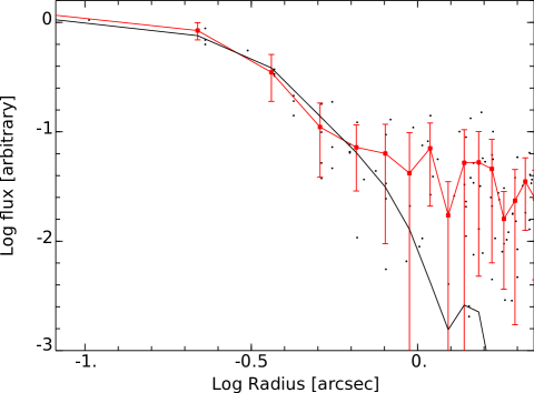
Figure 5: Surface brightness profile of the nucleus between PA $-40$ and 110$\degr$. The individual pixels are represented by small dots. The average brightness (between $-40$ and $110\degr$) in consecutive annuli is marked by connected solid disks. The other line is the scaled profile of a field star.

3.2.2 Thermal model

In order to examine the possibility of ice sublimation being the driver of the observed dust ejection features, we treat the object as a comet nucleus. As such, the question is how long will ice survive in the interior of such a small object at such a small heliocentric distance. For the purpose of modelling the thermal evolution of the nucleus, we assume a similar 1-D model and numerical implementation to that described in detail by Prialnik (1992) and Sarid et al. (2005). Further discussion of the input physics can be found in Prialnik et al. (2004).

A comet nucleus is generally portrayed as a porous aggregate of ices and solids (Weidenschilling 2004). The internal structure can be modeled as an agglomeration of grains made of water ice (and perhaps other minor volatile compounds) and solids (silicates, minerals) at some mixing ratio, with a wide spread in the size distribution of the components. The ice more volatile than water are neglected in our treatment as any such ice becomes depleted during a long term evolution, even down to the core of much larger objects (see Prialnik & Rosenberg 2009). Furthermore, if the object originated in the asteroid belt, it is more likely that H₂O ice would be crystalline and that the initial abundance of more volatile ices would be minute (e.g. Meech & Svoren 2004). We solve the set of coupled, time-dependent equations of mass conservation (dust, ice and vapor components) and heat transfer (see Prialnik et al. 2004, for a detailed description). The boundary conditions for these evolution equations are vanishing heat and mass fluxes at the center, vanishing gas pressures at the surface and a requirement for energy balance at the surface:

$$F(R) = \epsilon\sigma T(R,t)^{4}\,+\,$$ (1)

$$P_{\rm vap}(T)\sqrt{\frac{\mu}{2}\pi R_{g}T}H-(1-A){L_{\odot}\over 4\pi r(t)^{2}}\cos\xi,$$

where $\epsilon$ and $A$ are the emissivity and surface albedo of the nucleus, $L_{\odot}$ is the solar luminosity, $\sigma$ is the Stefan-Boltzmann constant, $R_{g}$ the molar gas constants and $\mu$, $P_{\rm vap}$ and $H$ are the molar mass, vapor pressure and sublimation latent heat for water. This condition on the surface flux, $F(R)$, depends on the Temperature $T$ , heliocentric distance $r$ and local solar zenith angle $\xi$ and is calculated for each time step. The first term corresponds to the re-radiated heat, the second to the sublimation, and the third the absorbed solar radiation. Without any additional information, we assume a fast rotator with the sub-solar point illuminated at perihelion.

We consider two cases for this object: “Case I”, which is similar to an S-type asteroid, and “Case II”, which is taken as a comet nuclei. Using the assumptions and measurements described in the previous section, Case I has a radius, bulk density and albedo of 85 m, 3000 kg m^-3 and 0.11, respectively. Case II has a radius, bulk density and albedo of 130 m, 1000 kg m^-3 and 0.04, respectively. If we assume the solid component (both the nucleus and the dust) to have specific density similar to that found for the dust particles of comet Wild 2, $\sim$ 3400 kg m^-3 (Kearsley et al. 2009), we can constrain the initial ice abundances for the thermal evolution calculations (see Prialnik et al. 2008). These values are taken as 0.05 and 0.5 (with corresponding initial porosities of 0.01 and 0.3) for Case I and Case II, respectively. All other physical parameters are taken to be similar to the Prialnik & Rosenberg (2009).

Our simulations of the nucleus evolution are run until the water ice component is depleted from the interior. For Case I (“asteroid”), there is no more water ice present after $\sim 3\times 10^{5}$ yr, while for Case II (“comet”) water ice becomes negligible and is buried deep under the surface after several $10^{6}$ yr. This is shown in Fig. 6a, where the sub-surface water ice depth is plotted as a function of time. Beyond this point in time, the water ice component is rapidly depleted, as the innermost layers reach a temperature of 200 K and 180 K, for Case I and Case II respectively. This is shown in Fig. 6b, where the evolution of the central temperature is plotted, for both cases, up to $10^{7}$ yr. The penetration of heat into the interior and the rise of the innermost temperature is slower for Case II and the final temperature reached is lower throughout most of the evolution time. Case I heats up faster because it is less porous (bulk density is higher) and has a much larger mass fraction of dust (silicates and minerals), so heat diffusion is less attenuated by sublimation.

In summary, considering a comet-like and an asteroid-like cases for the composition and structure of the nucleus, our thermal modelling efforts indicate that the interior reaches a temperature over 180K in a few $10^{5}$ to a few $10^{6}$ years. The nucleus would therefore be fully depleted of water ice —and any other more volatile ice— in that time scale. The orbit of P/2010 A2 is typical of an inner Main Belt asteroid, possibly member of the Flora family, with no indication that it would have been very recently injected or captured from a location more distant from the Sun. The survival depth of water ice becomes greater than $\sim 10\%$ of the object’s radius in less than a million years, almost independent of the initial choice of model parameters. This model therefore indicates that ice sublimation could not play any role in lifting dust from the surface of the object or dragging any substantial amount of grains from the interior. In what follows, we will therefore assume that the nucleus of P/2010 A2 has the characteristics of a Flora family, S-type asteroid, as detailed in this section and the previous one.

a.
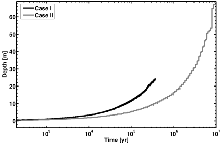
b.

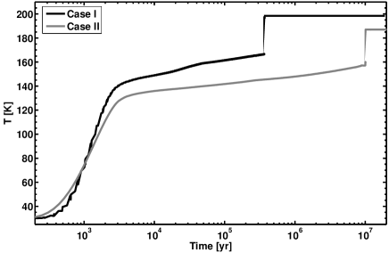
Figure 6: Evolution of the water ice sublimation front and the central temperature for the nucleus of P/2010 A2. The x-axis represents the time [yr] in log scale since the placement of the object in its current orbit, the y-axes represent: a. The sub-surface depth where crystalline ice survives; b. The central temperature. Case I (“asteroid”) is plotted in black, while Case II (“comet”) is plotted in gray.

3.3 Dust and the tail

3.3.1 Dust dynamical modelling

The dust tail was modeled using the Finson-Probstein (FP) dust dynamical method (Finson & Probstein 1968), modified by Farnham (1996).

Dust is extracted from the nucleus, by gas drag in traditional sublimation-driven cometary activity, or via direct ejection in the case of an impact. The dust is decoupled from the gas flow (if any) within a few nuclear radii, and is no longer influenced by the nucleus gravity, which becomes negligible. The motion of a refractory dust grain will then be defined by its initial velocity and affected by the solar gravity and radiation pressure, both acting in opposite radial directions. The net result of the two influences may be thought of as a reduced gravitational force acting upon the dust. The parameter $\beta$ is defined as the ratio of the radiation pressure force to the gravitational force, and is given by

$$\beta=5.740\times 10^{-4}\frac{Q_{\rm pr}}{\rho a}$$ (2)

for grain of radius $a$ [m] and density, $\rho$=3 000 kg m^-3. $Q_{\rm pr}$ is the radiation pressure efficiency (typically 1–2, depending on the material scattering properties).

The FP method involves computing the trajectories of dust grains ejected from the nucleus at velocity $v$ and under the influence of solar gravity and radiation pressure. A collection of particles of different $\beta$ ejected at a particular time follow trajectories called synchrones, while a single particle size ($\beta$) ejected over a range of times follow trajectories called syndynes. The combined set of curves maps out the expected ejected dust distribution. The extent to which the actual dust surface brightness correlates with the syn-curves may be used to infer which grain sizes are present, the onset an duration of activity, and any initial ejection velocity.

In order to investigate the origin of the dust tail, rather than starting with an entirely generic model which would have a large number of loosely constrained free parameters, we proceeded by steps, focusing on some aspects of the tail and making some simplifying hypotheses.

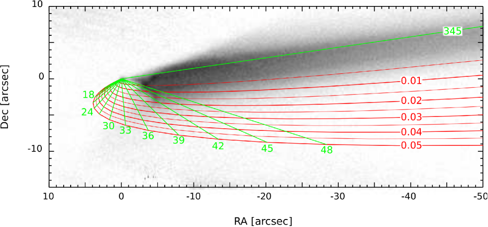
Figure 7: Syndynes (labeled with $\beta=0.01$–$0.05$) and synchrones (labeled in days since emission, 18–345) for dust grains emitted from the nucleus with zero velocity. The background image if from Fig.2.e.

3.3.2 Tail morphology and duration of the activity

Overlaying the syndyne and synchrone curves onto the image of the comet (see Fig. 7), it is clear that the region corresponding to dust emission during the 30 days before the observations is completely empty of dust. Together with the negligible contribution from the dust to the near-nucleus area, this confirms that any cometary activity must have stopped at least several weeks before the observations.

The light bridge connecting the nucleus to the tail matches the position expected for very large dust grains. Jewitt et al. (2010) measured the orientation of the tail on the high-resolution HST images, concluding that there was a short period of dust emission between Feb. and Mar. 2009.

However, while the orientation of the tail corresponds well to the direction of that synchrone, its position is offset from what is expected from a dust emission a zero speed from the nucleus. Also, the position of the northern fin is not matched by any syndyne, and the constant appearance of the tail while the Earth passed through the orbital plane indicates a more complex, 3D geometry and dust emission with non-zero velocities.

We will now further investigate the dust release characteristics. Adding up the scattered light from a distribution of dust particles emitted from the nucleus over a range of times as it moves away from the object, one can build synthetic images of the corresponding tail. Comparing the surface brightness of the synthetic tail to the real data, observational data can be inverted and information about the grain size distribution, ejection velocity and onset and cessation of activity can be obtained.

Various general dust emission models were explored to investigate the overall morphology of the tail. The first model included emission for a long duration of time, about a year from the time of observation to three months before the observation. The second model included only one month of emission beginning a year prior to the observation. Finally, a third model only included a single burst of emission one year before the observation. The emission takes place at the sub-solar point, with a constant dust production during the considered period. The dust size range and distribution and emission velocities were adjusted so that the reconstructed tail reproduces as well as possible the observations. The parameters are adjusted to reproduce the orientation (measured by its position angle) and width (measured perpendicular to the tail) of the tail, and the surface-brightness distribution along the tail. The actual position offset between the tail and the nucleus is not measured at this stage; it is considered as an effect of the global/average emission velocity, and will be dealt with later.

The best parameters for each model are listed in Table 4, the corresponding reconstructed images are shown in Fig. 8 and the surface brightness profiles are displayed in Fig. 9. These profiles were obtained by averaging 52 pixels perpendicularly to the tail on an image rotated by 8$\degr$ so to have the tail along the X direction. The first two models failed to reproduce the overall width, shape and/or brightness profile of the tail, even for the best adjustment of the parameters. While it may not be obvious from Fig. 8, the light distribution along the length of the tail is very different for models 1 and 2 compared to the reference image, as seen in Fig. 9.

The third model, with a single burst of emission, reproduces well these shape, width and profile of the tail with the particle sizes in the $a=1.5$ to 20 mm range, with a size distribution proportional to $a^{-3.5}$. The low end of the range is set by the edge of the image, and the upper end corresponds to particle with a minimal sensitivity to the radiation pressure.

The parameter values for Model 3 are tightly constrained in the adjustment process: power laws shallower (-3.75) or steeper (-3.25) fail to reproduce the profile of the tail. The best range of speeds of the particles was 0.20 to 0.30 m s^-1, with smaller particles having higher velocities. The range of particle speeds that still develop an acceptable model is only 0.10–0.40 m s^-1. The total emission can vary by less than a factor of 2 and still acceptably reproduce the observed surface brightness. The total amount of mass ejected (assuming a density $\rho=$ 3 000 kg m^-3 and albedo $p=0.11$) was about $5\times 10^{8}$ kg, again within a factor of 2.

In summary, reproducing the overall morphology of the tail suggests that the dust was emitted during a single burst about one year before the observations. The dust grain distribution follows a power law in -3.5 in the 1.5–20mm range, emitted with slow velocities in the 0.20–0.30 m s^-1 range.

We also note that, for a water-ice sublimation-driven dust emission, Delsemme (1982) obtains for an object at $r\sim 2$ AU ejection velocities in the 0.3–0.4 km s^-1 range, i.e. over 3 orders of magnitude larger than the velocities obtained in the FP modelling. However, the assumptions made by Delsemme are not necessarily valid here, so we will not use this argument.

Moreno et al. (2010) analyzed a set of images obtained between 14 and 23 Jan. 2010 using a different modelling technique, assuming particles ranging between 0.01 and 10 mm with a density of 1000 kg m^-3 and an albedo of 0.04. Their best fit suggests dust emission lasted over several months, ending just after perihelion (Dec. 2009), with a complex emission function over that period. While their model was richer than ours in terms of the complexity of the emission pattern, our first FP analysis cannot support that there was dust emission that late (see Fig. 7). Our model that is closest to their best fit is Model 1 (although ours uses a constant emission). Our Model 3, with an burst emission, reproduces the tail much better. Jewitt et al. (2010) concluded from the evolution of the tail position angle over 25 Jan.–29 May. 2010 that the dust had been emitted in a brief burst around 2 Mar.2009, plus or minus a few weeks. Snodgrass et al. (2010), taking advantage of the different viewing geometry from the Rosetta spacecraft, concur that the emission was very short, further constraining the emission date to 10 Feb. 2009, plus or minus 5 days.

Model 3 nicely reproduces the overall morphology of the tail, in particular its orientation and width, and the detachment from the nucleus and the overall surface brightness profile. However, it fails to reproduce the sharp edges and features visible in the head. Using the results from this model, we will further investigate the hypothesis of a single burst of emission.

Table 4: Three FP models

Model	1	2	3
Emission period,
starting on 10 Feb. 2009	250 days	30 days	1 day
Particle size range (mm), $a$	0.3–3	1.5–100	1.5–20
Particle size distribution power	-1	-3.9	-3.5
Emission velocities (m/s)	0.20-0.30	0.10-0.20	0.20-0.30
Fidelity of the model	Poor	Very poor	OK

Note: the emission duration is set, the other parameters are adjusted to reproduced the observed tail.

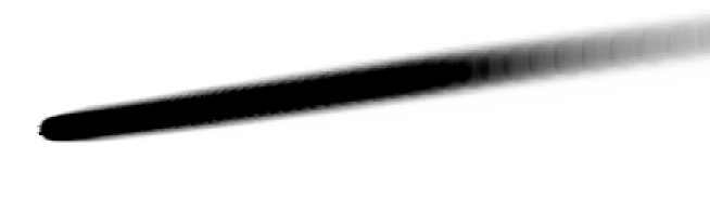
a. b.
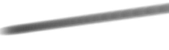
c.
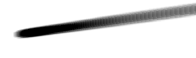
d.

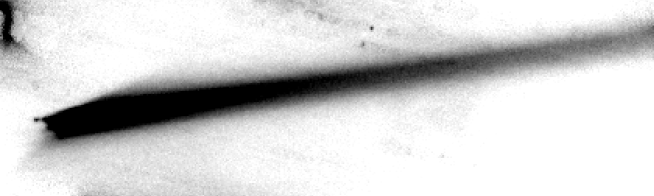
Figure 8:   Synthetic image of P/2010 A2, a. for the best fit with a long period of dust emission (Model 1, in Table 4). b. for the best fit with a month-long period of dust emission (Model 2). c. for the best fit with single burst of dust emission (Model 3). d. Reference image, same scales. This is the same image as Fig. 2.e.

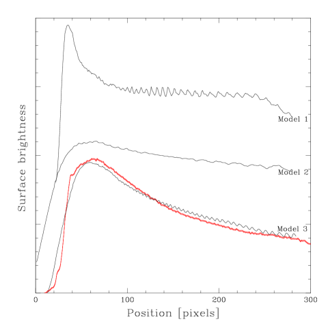
Figure 9: Photometric profile of the reference image (bold line) and the three models. Model 1 was shifted vertically for clarity.

3.3.3 Quantity of dust in the tail

The presence of striae in the tail is usually a sign that secondary dust emission is taking place, for instance from sublimating grains in traditional comets. It is also a warning that basic FP modelling should be applied with extreme care. In the case of P/2010 A2, however, the situation is actually simpler. Considering the bright knots in the arcs as the secondary dust grain source giving birth to the corresponding striae, the straight striae emanating from the knots follow synchrone curves. The range of emission epoch compatible with the observations is measured esitimating (by eye) the range of position angle that fit that of the striae. This range corresponds to emission taking place $340^{+30}_{-20}$ days before the observations, i.e. in agreement with the epoch of the main event. We conclude that each stria corresponds to dust grains with a distribution of $\beta$, ejected from the nucleus at the same time of the main dust release, with the same velocity as the material in the knot leading the stria. The surface brightness distribution as a function of the distance to the arc constitutes therefore a “dust grain radius spectrum” of the material.

We wish to estimate that dust size distribution, as well as the total quantity of dust in the tail, using the sky-subtracted, flux calibrated composite image from 19 Jan. 2010 (the deepest image). For each pixel we want to know which fraction is covered by dust (filling factor $f$), multiplied by the albedo ($A$). $Af$ is a convenient dimension-less equivalent to the surface brightness. Using the formalism of A’Hearn et al. (1984) we convert the measured flux in $Af$, ie.

$$Af=\left(\frac{2\Delta_{\rm km}r_{\rm AU}}{\rho_{\rm km}}\right)^{2}\frac{F_{{\circ\!<\!\!\!\!\!\!\ -\!\!\!\!-}}}{F_{\sun}}\leavevmode\nobreak\ ,$$ (3)

$\Delta_{\rm km}$ is the geocentric distance in km, $r_{\rm AU}$ the heliocentric distance in AU, $\rho_{\rm km}$ the linear size of the aperture at the distance of the comet (in km), $F_{\circ\!<\!\!\!\!\!\!\ -\!\!\!\!-}$ the measured flux of the comet, and $F_{\sun}$ the flux of the Sun at 1AU. Converting Eq. 3 for square pixels ($p$ arcsec), and expressing ${F_{\circ\!<\!\!\!\!\!\!\ -\!\!\!\!-}}/{F_{\sun}}$ in CCD ADUs, it becomes

$$Af=\frac{4\pi r^{2}}{(4.848\times 10^{-6}p)^{2}}10^{-0.4(ZP-k(z-1)-M_{\sun})}\,{\rm ADU}_{\circ\!<\!\!\!\!\!\!\ -\!\!\!\!-},$$ (4)

where $ZP$ is the zero point, $z$ the airmass and $k$ the extinction coefficient (in mag/airmass; Gemini’s ZP is expressed for 1 airmass, $ZP=28.20$ from Section 2.2).

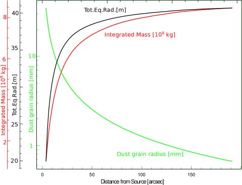
Figure 10: The labeled curves show, as a function of the distance to the arc-shaped features in the head of the tail, the radius of the dust particles [mm], the integrated mass in the tail out to that distance [kg] and the radius of the sphere of equivalent volume [m]. Refer to the text for the assumptions that were used to derive these values.

In order to count the number of dust particles in each pixel, we estimated the size of the particles, assuming that all the dust in the tail was emitted during a single burst that took place on 10 Feb. 2009 (using the date of Snodgrass et al. (2010), see 3.3.2), with a zero velocity from the large chunks of material that ended up located in the arcs. The apparent distance from the arcs to the particle is then a measurement of $\beta$, the conversion factor is estimated running our FP code for particles over a range of values of $\beta$ for an emission date in Feb. 2009. Using the relation between $\beta$ and the characteristics of the particle from Finson & Probstein (1968), we convert $\beta$ in the radius of the particles, $a$, using Equation 2. We use $Q_{\rm pr}=1$, as Moreno (2009), for large absorbing grains (Burns et al. 1979). We assume a density of 3 000 kg m^-3 (see Section 3.2.1). Figure 10 displays the corresponding sizes, ranging from few tenths of millimetres at the edge of the frame to few millimetres close to the arcs. Using the formalism of Agarwal et al. (2007), the dust size distribution inferred from the surface brightness profile along the tail is a power law in the $a=1$–20 mm range, with a number of particles proportional to $a^{n}$ (differential size distribution), with $n={-3.44\pm 0.08}$. This value is in agreement with that modeled in the previous section, and with those reported by Moreno et al. (2010), $n=-3.4\pm 0.3$, Jewitt et al. (2010), $n=-3.3\pm 0.2$ and Snodgrass et al. (2010), $n=-3.5$. A value close to -3.5 is significant because this is in agreement with the empirical value for the distribution of particle sizes resulting from a collision, and for a collisionally relaxed population (Dohnanyi 1969). The value for the dust in the tail of P/2010 A2 is slightly steeper than the size distribution measured with Hayabusa for the boulders larger than 5 m on the surface of (25143) Itokawa, $n=-3.1$ (Michikami et al. 2008).

The total $Af$ is measured in a series of thin rectangular apertures as long as the width of the tail and covering it from the arcs until the edge of the frame. The total $Af$ is converted into a number of particles using the radius $a$ of the particle at that distance from the arcs as computed above.

The total mass and volume of dust is integrated by adding the contribution of each rectangular aperture starting from the arcs. The mass integrated along the tail, as well as the volume of the corresponding sphere are displayed in Fig. 10.While there is still a significant amount of dust in the tail extending beyond the edge of the frame, the asymptotic behaviour of the growth curve indicates that a very large fraction of the mass is present in the visible part of the tail. With these assumptions, we estimate that the tail contains at least $8\times 10^{8}$kg of ejected dust, which could be re-assembled into a sphere of radius $r_{e}\sim 40$ m.

Jewitt et al. (2010) reached similar estimates based on the analysis of their Hubble images: 6–60$\times 10^{7}$ kg, corresponding to a sphere with a radius of at least 17–36 m. The latter corresponds to a distance of 20^′′ from the arcs on Fig. 10, which is about where the S/N starts to degrade on their Hubble images: we consider their larger estimate in agreement with ours. The total ejected mass is likely to be higher, as these values poorly estimate the size and number of large particles in X-shaped arcs.

3.3.4 Envelope of the tail

A dust emission model was developed to investigate the possible cause of the position of the tail behind the X-shaped arcs, and its distinct detached geometry. For this investigation, rather than trying to reproduce the light distribution in detail using a general fit of the dust velocity vector ${\bf v}_{\rm d}$ and $\beta$ distributions, a greatly simplified model was implemented as follows. The details of the model, of its implementation and of its results are beyond the scope of this paper, and constitute a separate, companion paper (Kleyna et al. 2011).

The dust emission is represented by an instantaneous burst on 10 Feb. 2009 (date from Snodgrass et al. 2010, see 3.3.2). The first simplification represents the emission geometry with a cone (defined by its half-opening angle $\alpha_{\rm c}$ and axis orientation), on which dust grains characterized by a distribution of $\beta$ are emitted with a distribution of velocity $v_{d}$. The motion of the dust grains is computed taking into account the Sun’s gravity and the radiation pressure to determine their final positions in the image plane at the time of the observations.

The second simplification is to only consider whether the dust grains fill the envelope of the observed tail, completely neglecting the light distribution within that envelope. The envelope is defined visually on the images of 19 Jan. (Fig.2.e), so as to enclose the main tail. Several different plausible envelopes, estimated by eye, were defined to test the dependency of the result on the choice of the envelope. This allows us to neglect the actual distributions of $\beta$ and $v_{\rm d}$: only the minimum and maximum values are relevant to the model. The natural minimum velocity and minimum dust size are zero; the dust size is assumed to be independent of the velocity (this is supported by experimental studies of impact onto porous, regolith-like material, which are appropriate for gravity- or weak cohesive strength-controlled craters which, as we discuss later, seems to be the case here). Finally,the only difference between a filled emission cone and a hollow one is the presence of a cap at the open end of the cone, we can therefore further simplify the model considering a hollow cone.

This leaves only four free parameters: the two coordinates defining the orientation of the cone axis, the cone half-opening $\alpha$, and the maximum dust velocity $v_{\rm d,max}$. The merit function of a set of parameters is computed by assigning penalty to dust grains ending up outside of the envelope of the tail, and to pixels within the tail that contain no dust grain. Kleyna et al. (2011) describes the exploration of the four parameter space, the method used and the sensitivity to the definition of the envelope. Only a fairly narrow subset of the parameter space can reproduce the observed tail envelope. The best model is a cone (either full or hollow) with a half-opening of $40\degr$, pointing below the orbital plane and on the forward side of the comet, with a maximum dust velocity of 0.2 m s^-1. The direction of the emission is strongly constrained by the position of the tail with respect the nucleus and by the sharp edge of the head.

3.3.5 Arc-shaped features

In order to investigate the origin of the arc-shaped features (see Fig. 3), another model was implemented; it is also described in detail in Kleyna et al. (2011). Each arc appears as a one-dimensional feature; they are not parallel to the synchrones for the date of the dust emission (see Fig. 7, position angle near $278\degr$). They can therefore not be caused by the radiation pressure-driven spread of particles with a range of $\beta$; they must therefore correspond to very large particles very weakly sensitive to radiation pressure (i.e. with $\beta=0$).

A large number of particles were modeled, with an emission date on 10 Feb. 2009 (date from Snodgrass et al. 2010, see 3.3.2), sampling the emission direction and velocity space. The motion of these particles was then computed until the date of the observations, and their position in the image plane computed. Those landing on position of the arcs are marked. Only particles with a ejection velocity $v_{\rm d}>0.20$ m s^-1 can contribute to the X-shaped arcs, but this model cannot set an upper limit. Indeed, dust grains with higher emission velocity can be emitted and end up further away from the nucleus at the time of the observation, but still appearing in the same position in the image due to foreshortening. Test particles from two regions in the (velocity, direction) space end up in the position of the arcs. The arcs could therefore have been produced by dust grains from one of these region, the other, or a combination of both.

However, one of these regions is found to match a section of the surface of the cone modeled to describe the overall tail in the previous section: the direction of emission and velocity are identical. This suggests that the same hollow cone (with its orientation, opening and emission velocity) describes both the overall tail geometry as well as the arcs in the head of the tail. The former corresponding to small dust grains subjected to radiation pressure, the latter corresponding to a fraction of the large dust grains populating the propagated cone. Only a fraction of the large dust grains are visible as arcs, as the geometry at the time of the observations gives a foreshortened side view of a segment of the cone. The other large dust grains appear diluted over the tail.

Observations from another point of view should show other features fortuitously aligned along that other line of sight. Unfortunately, the Rosetta images (Snodgrass et al. 2010) do not have a sufficiently high resolution to reveal them: all the region presenting structure was contained in one single pixel of the Osiris Narrow Angle Camera on Rosetta. In this context, the striae visible in the tail (see Fig. 3 and 4) simply correspond to irregularities of the emission along the cone.

3.3.6 Fin-shaped features

The position of the North fin, above and beyond the asymptotic direction of the synchrone in Fig. 7, suggest an out-of-plane feature, in turn indicating an out-of-plane ejection velocity vector. It can be explained as a consequence of the ejection cone described in the previous section. The cone itself defines the left edge of the fin, the smaller dust being driven back to create the body of the feature. The SE fin could not be reproduced.

3.4 Alternative emission processes

When evaluating the characteristics of the nucleus, in Section 3.2.2, we concluded that no water ice or more volatile species would have survived for more than a few million years in the body on its current orbit. This makes cometary activity a very unlikely cause for the observed dust emission, as it would require a mechanism to inject the object on its current Flora-like orbit in the recent past.

The FP modelling of the tail (Section 3.3.1) and other studies (Jewitt et al. 2010; Snodgrass et al. 2010) firmly indicate the emission duration was very short, in the form of a burst that took place around Feb. 2009. The more detailed dynamical dust models presented in the previous section suggest this emission took place on a cone with an half-opening $\alpha=40\degr$. As we will discuss in the following section, this strongly suggests that the dust emission corresponds to an ejecta cone resulting from an impact with a smaller body. In this section, we shall briefly consider other alternative dust emission processes: rotational spin-up and electrostatic dust levitation.

Rotational spin-up

: Small objects in the main belt can be driven toward rotational instability by radiation torque Rubincam (2000). Radiation torque can spin-up or spin-down the object depending on its shape and the nature of the object, and the numerous small asteroids that are either fast and slow rotators suggest this effect is indeed acting widely (Pravec & Harris 2000). However, simulations indicate that the ejection of material from a spun-up object occurs along the equatorial disk (Walsh et al. 2008), i.e. with a geometry that is very different from what is observed here. These numerical simulations were done for particles larger than dust. However, the geometry of the large grains observed in this object seems completely incompatible with the rotational spin-up lifting.

Electrostatic lift:

Spacecraft have observed fine particles levitated at velocities near 1 m s^-1 at the Moon’s terminator caused by the buildup of a potential difference between illuminated and shadowed regions (de Bibhas & Criswell 1977). On small asteroids, this effect can launch dust above the local escape velocity (Lee 1996), creating visible mass loss. However, there are thousands of asteroids similar in size to the MBCs that do not eject observable dust. Furthermore, the FP analysis of the dust around P/2010 A2 indicates it is constituted of large dust grains, which could not be lifted up by electrostatic force.

3.5 Physical implications of ejecta geometry

One remaining source of the observed release of dust is the excavation of material from an impact on the nucleus. In this section, we demonstrate to first order that an impact event is consistent with, and could explain, the three main requirements from observations: the duration of release, velocity distribution and provenance, and amount of mass. We restrict our analysis to a canonical vertical impact here, although impacts at normal incidence rarely occur on planetary objects; instead, the vast majority occur obliquely for both spherical (Gilbert 1893; Shoemaker 1963) and asteroidal-type bodies (Cheng & Barnouin-Jha 1999).

In a hypervelocity impact event, strong shockwaves and subsequent rarefaction waves set material in motion, excavating and ejecting a portion of the displaced target up and out of the crater; the remainder of the displaced mass remains compressed in the target. In general, the velocities of main-stage ejecta can be described by a power-law relationship with either time or launch position, as dimensionally predicted (e.g., Housen et al. 1983), and demonstrated by a number of experimental (e.g., McGetchin et al. 1973; Schultz & Gault 1979; Piekutowski 1980; Oberbeck & Morrison 1976; Piekutowski et al. 1977; Cintala et al. 1999; Anderson et al. 2003) and numerical studies (e.g. Wada et al. 2006). The ejection angles of ejecta are a function of the material properties of the target. In granular target materials (like regolith, as expected on an asteroidal surface), ejection angles (referenced from local horizontal) $\psi=90\degr-\alpha_{\rm c}$ range from $\sim 30\degr$ to $\sim 50\degr$ (Cintala et al. 1999; Anderson et al. 2004; Anderson & Schultz 2005; Hermalyn & Schultz 2010) with an average $\alpha_{\rm c}\sim 45\degr$ (Housen et al. 1983) and evolve throughout crater growth. In cohesive targets (such as solid basalt or a welded material), ejection angles tend to be considerably higher ($\psi\sim 70\degr$ Gault 1973). Additionally, highly porous material exhibits a high-ejection angle component (Schultz et al. 2007). Our finding of an $\alpha_{\rm c}=40\degr$ hollow cone is in agreement with an impact into an unconsolidated, granular target. The progression from lower ejection angles (larger $\alpha_{c}$) for faster velocity material to higher ejection angles (smaller $\alpha_{c}$) at later times and slower velocities is consistent with the ejection angle evolution in experiments and computations for unconsolidated granular material (Hermalyn & Schultz 2010, 2011).

Crater growth is arrested either when the ejecta velocities are insufficient to launch material above the crater rim (gravity-controlled) or when the shock strength drops below the yield strength of the material (strength-controlled). The cutoff in velocity solution space of $\sim 0.10$ m s^-1 is coincident with the escape velocity of the body. Therefore, any material ejected under this velocity component could have returned to the surface of P/2010 A2 and no record of this material would be apparent in the images. This behavior would be consistent with a gravity-scaled crater. Alternatively, if the surface exhibits a degree of material strength, crater growth could be arrested with virtually no ejecta launched below the 0.10 m s^-1 cutoff. We note that although it is impossible to separate the effects of gravity and strength controlled crater arrestment without watching the evolution of the ejecta curtain. Since both gravity and strength are inferred to be weak, both probably play a role in the termination of growth. It is possible to define a theoretical gravity-controlled crater radius as a limiting size since ejection velocities during main-stage growth will be unaffected by the difference in termination processes.

In Section 3.3.3, we concluded that the visible ejecta corresponds to a sphere with a radius $r_{e}\sim 40$ m. Jewitt et al. (2010) estimated $r_{e}$ in the 17–36 m range. In both studies, the dust particles were found in the 2–20 mm range, which further supports the excavation of fine regolith-like material in a gravity-scaling regime. To approach the size of the crater, we look to the ejected mass as a constraint. The total amount of mass ejected from a crater tends to only be approximately 50% of the total displaced mass (e.g. Stöeffler et al. 1975; Croft 1980). The cumulative (and incremental) ejected mass above a certain velocity similarly follows a power-law relationship with velocity such that the vast majority of material is ejected at low velocities near the crater rim. The form of this equation for purely gravity-scaled craters is (as given in Housen et al. 1983):

$$\frac{\sum V_{e}}{R^{3}}=0.32\left(\frac{v}{\sqrt{gR}}\right)^{-1.22\pm 0.02}$$ (5)

where $V_{e}$ is the cumulative volume of ejecta with higher velocity, $R$ is the final gravity-scaled crater radius, $v$ is the velocity of ejecta, and $g$ is the gravity on the surface; the exponent and coefficient are fit to data from small-scale explosion and impact experiments into granular targets. Using the higher density values defined above, a crater approximately 100m in radius is required to eject sufficient material above escape velocity to match the observed minimum ejected mass (see Fig. 11). The total time to eject the observed material would be on the order of seconds. A strength-controlled crater follows a similar relationship (see Housen et al. (1983) for details), but would require a much larger crater to eject the measured volume of material for anything other than extremely small values of material strength $Y$. Considerably larger craters are probably not physically possible on such a small body since even the gravity-scaled limiting radius is on the order of the radius of the body itself. However, there are other bodies that exhibit craters or large-scale depression features of radii approaching that of the body itself; e.g., Mathilde, Phobos and Deimos, Gaspra, and even the Moon.

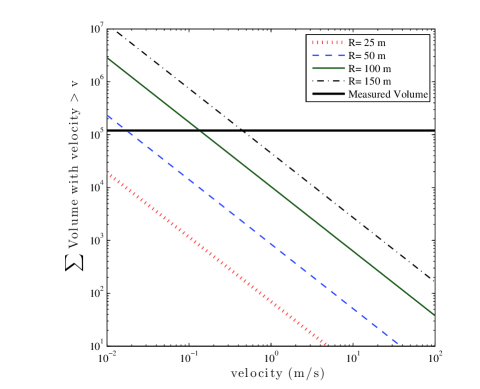
Figure 11: Cumulative volume of ejecta with higher velocity for a set of crater sizes in the gravity-scaled regime. Measured volume of material is indicated by solid black line. A crater approximately 100m in radius is required to excavate sufficient material above the escape velocity of the body to match observations.

One possible mechanism that could help explain the development of such large craters without catastrophically disrupting the body is an oblique impact, which decreases the peak shock pressures while still excavating a large amount of material (Schultz 1997; Cheng & Barnouin-Jha 1999; Schultz, P. H. & Crawford 2011). This process could also explain the enhancement of higher velocity material ($>0.25$ m s^-1) in the images, since ejecta downrange (i.e., in the direction of impact) is enhanced in mass and velocity throughout much of crater growth (Anderson et al. 2003) and may appear strongly foreshortened in the images due to perspective. The body may also be fairly porous, which will serve to further attenuate the peak shock pressures.

4 Summary and discussion

The dust tail of P/2010 A2 was observed and analyzed so to cast some light on the possible cometary nature of that object, as its appearance and orbit could make it a member of the small family of Main Belt Comets. The main results and conclusions of this study are listed hereafter.

• Observations were acquired with GN, NTT, UH 2.2-m from 14 Jan. until 19 Feb. 2010. The tail did not show any measurable evolution over that time span, which included the crossing of the orbital plane, which indicates the tail is an out-of-plane 3D structure, suggesting the dust was released with a significant orthogonal velocity.

• The nucleus, detached from the tail, appears not to be surrounded by dust (at most 3% of the light corresponds to near-nucleus dust); dynamical dust models also indicate that no recent dust is present, suggesting no cometary activity at the time of the observations. The absolute magnitude of the comet was estimated to SDSS $r^{\prime}(1,1,0)=21.74\pm 0.04$ on 19 Jan. 2010 and $21.55\pm 0.05$ on 2 Feb. Assuming an albedo $p=0.11$, a value typical for S-type asteroids, this converts into a nucleus of radius $r=80$–90 m. Using a density of $\rho=3$ 000 kg m^-3 (also typical of a S-type asteroid), the escape velocity of the body is $v_{e}=0.10$–0.12 m s^-1.

• A thermal model of the nucleus indicates that water ice (as well as any more volatile ice) would not survive more than a few million years in the object on its current orbit. As we have no reason to suspect a recent insertion on the current orbit, this rules out ice sublimation as the source of the observed dust. Rotational spin up and electrostatic lifting were also rejected as possible source for the dust tail.

• A Finston-Probstein-type dynamical dust modelling of the morphology, light distribution and detachment of the tail indicates that a short burst of dust emission (a day long or less) represents best the observed tail, with an ejection velocity in the range $v_{e}=0.20$–0.30 m s^-1. The ejection date is in agreement with other studies of this object (Jewitt et al. 2010; Snodgrass et al. 2010); we continue this study using Snodgrass’ date, 10 Feb. 2009. The model, together with direct measurements of the tail within the camera’s field of view, indicate it is constituted of dust grains with radii $a$ ranging between a few tenths of millimetres to 20 mm, with a number of particles proportional to $a^{-3.44\pm 0.08}$ (differential size distribution index). The total dust content of the tail is estimated to at least $8\times 10^{8}$ kg, which could be packed in a sphere with a radius of 40 m (assuming the same density $\rho=3$ 000 kg m^-3 as above).

• The position and shape of the tail’s envelope was modeled as originating from dust emitted on a cone with a half-opening angle $\alpha\sim 40\degr$ pointing below the orbital plane, toward the forward direction, with a ejection velocity $v_{e}\leq 0.20$ m s^-1. The X-shaped arcs were modeled as a collection of large particles, with $v_{e}\geq 0.20$ m s^-1; they were independently found to be emitted on a section of the same hollow cone. The are seen as an arc as a consequence of the geometric foreshortening of the cone section (after one year of evolution); other sections of the cone, which are not foreshortened in the same way, contribute to the overall tail. The Rosetta observations (Snodgrass et al. 2010) did not see other sections of the cone as arcs because of the coarser resolution of its camera.

• Because ice sublimation, electrostatic lifting and rotational spin up were rejected as possible causes for the dust emission, and because of the very short release time and the geometry of the dust emission on a hollow cone with an half-opening angle $\alpha=40\degr$, we conclude that the dust release was caused by an impact by a small object.

• Considering the volume of ejected dust in the framework of a gravity-dominated crater formation process, a crater of $\sim 100$ m radius was produced in a total time of the order of seconds. While that crater is large compared to the body, other bodies show craters as large as themselves. An oblique impact —which is statistically the most likely— would explain how P/2010 A2 escaped complete, catastrophic disruption.

In summary, the tail of P/2010 A2 can be explained by an impact on a $\sim 80$–90 m asteroid. The impact released dust in a hollow cone, which evolved for about one year to form the observed dust distribution. The fine-grained dust formed a long tail that was extended by solar radiation pressure, and the large grains (un-affected by the solar radiation pressure) retained the conical shape. The viewing geometry revealed sections of that cone as the arcs in the head of the dust cloud. Therefore, what we witnessed was likely an event of collisional grinding within the Flora collisional family, and not a genuine, water-ice driven Main Belt Comet. With increasingly sensitive sky surveys covering larger fractions of the sky during each dark period, we can expect to detect more and more of these collisions, as illustrated by the recent discovery of the dust cloud around (596) Scheila. While the original goal of this project was to probe the water ice content in the asteroid main belt, its end result was the observation of a natural impact on a small asteroid.