Mean field mutation dynamics and the continuous Luria-Delbrück distribution

Abstract

The Luria-Delbrück mutation model has a long history and has been mathematically formulated in several different ways. Here we tackle the problem in the case of a continuous distribution using some mathematical tools from nonlinear statistical physics. Starting from the classical formulations we derive the corresponding differential models and show that under a suitable mean field scaling they correspond to generalized Fokker-Planck equations for the mutants distribution whose solutions are given by the corresponding Luria-Delbrück distribution. Numerical results confirming the theoretical analysis are also presented.

Keywords: Luria-Delbrück distribution, kinetic models, mutation rates, Fokker-Planck equations

1 Introduction

Application of tools from nonlinear statistical physics to describe different biological phenomena started to gain popularity in the recent years and it represents one of the major challenges in contemporary mathematical modeling [4, 5, 11, 22]. In particular, powerful methods borrowed from kinetic theory of rarefied gases have been successfully employed to construct master equations of Boltzmann type, usually referred to as kinetic equations, describing the emergency of universal behaviors through their equilibria [7, 23, 26].

An important example of emergent behavior describes building of tumors by cancer cells and their migration through the tissues [5, 10, 11, 22]. Another famous example to consider in this contest is the classical Luria-Delbrück mutation problem [19, 31]. Certainly, the basic entities in these examples differ from the physical particles in that they already have an intermediate complexity themselves. However, for some specific phenomena, the statistical behavior of the system is related to the peculiar way entities interact and not to their internal complex structure.

First experimental and theoretical analysis of mutation process in bacteria was published by Luria and Delbrück in 1943 [19] (Nobel Prize in Physiology and Medicine, 1969). The goal of the study conducted by Luria and Delbrück was to estimate the mutation rate in bacterial populations by observing the fraction of the final cells that carry a mutation. In their experiment, often called fluctuation test, they have shown that in bacteria, genetic mutations arise in the absence of selection, rather than being a response to selection. They explained these results mathematically by the occurrence of a constant rate of random mutations in each generation of bacteria growing in the initial culture.

The distribution of the number of mutants in a culture that has been grown under conditions in which these mutations did not confer a selective advantage to the cells bearing them, came to be known as the Luria-Delbrück distribution.

In multicellular organisms, connection between mutagenesis and carcinogenesis is broadly accepted (see, for instance, [24]) and the Luria-Delbrück distribution plays an important role in the study of cancer, because tumor progression depends on how heritable changes (mutations) accumulate in cell lineages. In particular, the Luria-Delbrück model focuses on the distribution of mutations in an exponentially expanding clone of cells. We should mention here that several models describing the Luria-Delbrück experiment have been proposed. The most famous is the Lea-Coulson formulation [18] based on the introduction of a random rate of mutations instead of constant rate implemented in [19]. Other formulations have been introduced in [3, 2, 33]. We refer the reader to [31] for a comprehensive review of the subject. The mathematics behind the Luria-Delbrück experiment (most often in the Lea-Coulson formulation) has been studied by several authors [1, 12, 15, 16, 20, 32].

The specific shape of Luria-Delbrück distribution is strictly connected to the particular formulation of the mutation dynamics. In general, no analytic expressions of such distributions are available, however, exact expressions may be available for the characteristic functions, the probability generating functions and the moments. This indeed is the case of both the original (Luria-Delbrück) and the Lea-Coulson formulations considered in this manuscript. For such a reason a lot of effort has been invested in the development of computational methods and asymptotic approximations of Luria-Delbrück distribution (see [31] and the references therein).

Here we introduce kinetic master equations, in the spirit of [26], where the number of mutants is considered as a continuous variable instead of a discrete one. The behavior of the resulting differential models are then studied by using a suitable mean field asymptotic scaling, which permits to recover the exact moments of the original formulations. As the limit we obtain generalized Fokker-Planck equations and, for the classical Luria-Delbrück setting, show that the long time behavior is characterized by the corresponding Luria-Delbrück distribution. The same evidence is give numerically also for the Lea-Coulson setting.

The rest of the paper is organized as follows. In the next section we consider the standard Luria-Delbrück experimental settings and present the corresponding kinetic master equations. Then we introduce a mean field scaling that permits to derive a generalized Fokker-Planck model whose solution is given by the original Luria-Delbrück distribution of mutants. In section 3 we consider the case of a variable mutation rate as proposed by the Lea-Coulson formulation. Derivation of the generalized Fokker-Planck model for this case is also presented and its solution is discussed. Simple diffusion approximations of the mutation process are also derived in this section. Then, in section 4, we present numerical experiments confirming our theoretical analysis. Concluding remarks and possible extensions of this work are reported in the last section.

2 The Luria-Delbrück formulation

The mathematical formulation of the Luria-Delbrück model is based on the following assumptions

• The process starts at time $t=0$ with a number $N_{0}$ of normal cells and no mutants.

• Normal cells replicate at a constant rate $\alpha$.

• Mutation occur randomly at a rate characterized by a Poisson process with intensity proportional to the total number of normal cells. We denote with $\mu$ the mutation rate per cell.

• The offspring of every mutant cell replicate at a constant rate $\beta$.

As a consequence of the above assumptions if we denote by $N(t)$ the number of normal cells we obtain the differential problem

$$\frac{dN(t)}{dt}=\alpha N(t)-\mu N(t),\quad N(0)=N_{0},$$ (1)

which gives

$$N(t)=N_{0}e^{(\alpha-\mu)t},\quad t>0.$$ (2)

The fundamental question in the above model is the estimation of the distribution of the number of mutants in time. Such distribution, in fact, is of vital importance when estimating the mutation rates. We shall denote by $f(m,t)$ the probability density of having $m$ mutant cells at time $t$.

2.1 A kinetic model for mutations

In the sequel we will assume that the random variable $m$ characterizing the number of mutants at time $t$ takes values in $\mathbb{R}^{+}$. Such an assumption, as we will see later, permits us to tackle the problem with some tools borrowed from kinetic theory [6, 7, 23, 26]. Thus we have

$$\int_{\mathbb{R}^{+}}f(m,t)\,dm=1,$$

and denote by $M(t)$ the expected number of mutant cells at time $t$

$$M(t)=\int_{\mathbb{R}^{+}}f(m,t)m\,dm.$$ (3)

We consider the following microscopic dynamic for the random variable $m$

$$m^{\prime}=m+\beta m+\eta,$$ (4)

where $\eta\geq 0$ (absence of backward mutations) is a discrete random variable distributed accordingly to a Poisson density $p(N(t),\eta)$ with mean $\mu N(t)$.

By standard arguments we can write the following kinetic master equation for the time evolution of the distribution of mutant cells

$$\frac{\partial f(m,t)}{\partial t}=\sum_{i=0}^{\infty}\left[B_{{}^{\prime}m\to m}(N(t),\eta_{i})\frac{1}{J}f(^{\prime}m,t)-B_{m\to m^{\prime}}(N(t),\eta_{i})f(m,t)\right],$$ (5)

where ${}^{\prime}m=(m-\eta_{i})/J$, $J=1+\beta$, and the transition rates are given by

$$B_{{}^{\prime}m\to m}(N(t),\eta_{i})=p(N(t),\eta_{i})\chi(^{\prime}m\geq 0),\quad B_{m\to m^{\prime}}(N(t),\eta_{i})=p(N(t),\eta_{i})\chi(m^{\prime}\geq 0),$$

with $\chi(I)$ the indicator function of the set $I$. The above equation is complemented with the initial data

$$f(m,0)=f_{0}(m).$$ (6)

Since the random variable $\eta_{i}$ takes values only in $\mathbb{R}^{+}$ the weak form of the kinetic equation yields the simpler representation

$$\frac{\partial}{\partial t}\int_{\mathbb{R}^{+}}f(m,t)\varphi(m)\,dm=\sum_{i=0}^{\infty}p(N(t),\eta_{i})\int_{\mathbb{R}^{+}}f(m,t)[\varphi(m^{\prime})-\varphi(m)]\,dm,$$ (7)

where $\varphi(m)$ is a smooth function.

It is easy to see that taking $\varphi(m)=1$ we get the consistency condition

$$\frac{\partial}{\partial t}\int_{\mathbb{R}^{+}}f(m,t)\,dm=0.$$ (8)

The choice $\varphi(m)=m$ yields the evolution of the mean number of mutant cells and gives

$$\frac{\partial}{\partial t}\int_{\mathbb{R}^{+}}f(m,t)m\,dm=\sum_{i=0}^{\infty}p(N(t),\eta_{i})\int_{\mathbb{R}^{+}}f(m,t)[\beta m+\eta_{i}]\,dm=\beta\int_{\mathbb{R}^{+}}f(m,t)m\,dm-\mu N(t),$$

which corresponds to the simple ODE

$$\frac{dM(t)}{dt}=\beta M(t)+\mu N_{0}e^{(\alpha-\mu)t}.$$ (9)

The above equation can be solved exactly and, starting with initial data $M(0)=M_{0}$, gives

$$M(t)=\left\{\begin{array}[]{ll}\displaystyle\frac{\mu}{\alpha-\mu-\beta}N_{0}e^{(\alpha-\mu)t}(1-e^{-(\alpha-\mu-\beta)t})+M_{0}e^{\beta t},&\beta\neq\alpha-\mu,\\[14.22636pt] \mu N_{0}te^{(\alpha-\mu)t},&\beta=\alpha-\mu.\end{array}\right.$$ (10)

Note that the above expression for the mean coincides with what found in the literature for the Luria-Delbrück distribution [31].

Similarly we can compute the evolution of the variance. Starting from $\varphi(m)=m^{2}$ we have for the second moment $M_{2}(t)$ the equation

$$\frac{\partial}{\partial t}\int_{\mathbb{R}^{+}}f(m,t)m^{2}\,dm = \sum_{i=0}^{\infty}p(N(t),\eta_{i})\int_{\mathbb{R}^{+}}f(m,t)[\beta(2+\beta)m^{2}+\eta_{i}^{2}+2(1+\beta)m\eta_{i}]\,dm,$$

$$= \beta(2+\beta)\int_{\mathbb{R}^{+}}f(m,t)m^{2}\,dm$$

$$+ <\eta^{2}>+2(1+\beta)\mu N(t)\int_{\mathbb{R}^{+}}f(m,t)m\,dm,$$

where $<\eta^{2}>=\mu N(t)(1+\mu N(t))$ denotes the second moment of $\eta_{i}$.
Thus the variance

$$V(t)=\int_{\mathbb{R}^{+}}f(m,t)m^{2}\,dm-M(t)^{2},$$

follows the differential equation

$$\frac{dV(t)}{dt}=2\beta V(t)+\beta^{2}M_{2}(t)+\mu N(t)(1+2\beta M(t)+\mu N(t)),$$ (11)

which differs from the variance of the Luria-Delbrück distribution. The exact analytical solution to (11) can be easily computed, we omit it for brevity.

To analyze the long time behavior let us consider the case $N_{0}=1$, $M_{0}=0$, which represents the situation, where the mean numbers of normal cells and mutant cells are initially one and zero respectively (a standard Luria-Delbrück setup [19]). Note that, when the growth rates are identical $\alpha=\beta$, the average total number of cells is $B(t)=M(t)+N(t)=e^{\beta t}$ which is simply a birth process at rate $\beta$.

Let us define next the concentration of the mutant cells as $\rho(t)={M(t)}/{B(t)}$. The long time behavior of $\rho$ according to (10) is given by

$$\lim_{t\rightarrow\infty}\rho(t)=\begin{cases}1,~{}~{}&\beta\geq\alpha-\mu\;,\\ \displaystyle\frac{\mu}{\alpha-\beta},~{}~{}&\beta<\alpha-\mu\end{cases}$$ (12)

Figure 1: Long time behavior of mutant cell concentration as function of time

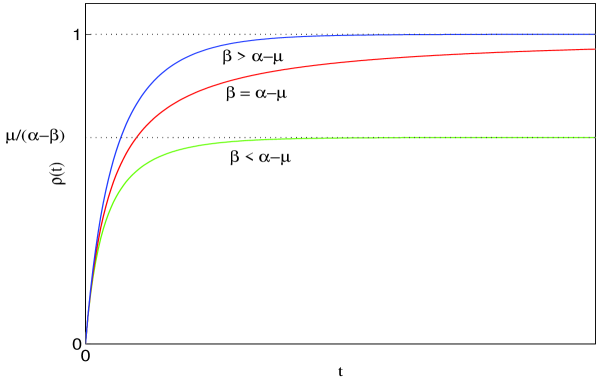
The behavior is sketched in Figure 1. Mutants become predominant when $\beta\geq\alpha-\mu$. It is interesting to revise that the asymptotic behavior of $\rho$ shows exponential convergence for all values of $\beta$ except for $\beta=\alpha-\mu$, where we have

$$\rho(t)=\frac{\mu t}{1+\mu t}$$

For $\beta<\alpha-\mu$ mutant cells represent a fraction $\mu/(\alpha-\beta)$ of the population and no predominant behavior is observed.

2.2 Derivation of the generalized Fokker-Planck model

In order to study the asymptotic behavior of the model we introduce the following scaling. We set

$${\tilde{f}}(m,\tau)=f(m,t),\qquad\tau=\varepsilon t.$$ (13)

We are interested in the behavior for small values of $\varepsilon$ such that

$$\lim_{\varepsilon,\beta\to 0}\frac{\beta}{\varepsilon}=\gamma,\quad\lim_{\varepsilon,\beta_{1}\to 0}\frac{\beta_{1}}{\varepsilon}=\gamma_{1}\quad\lim_{\varepsilon,\mu\to 0}\frac{\mu}{\varepsilon}=\nu,$$ (14)

where $\beta_{1}=\alpha-\mu$.

Roughly speaking the above scaling limit implies $m^{\prime}\approx m$ and corresponds to the realistic assumption of considering the the birth-mutation dynamic as a slow process originated by many small variations of the number of mutants. For this reason we will refer to the limiting dynamic as a mean field dynamic. In particular, as we will show, it is consistent with the evolution of the variance of the original Luria-Delbrück model.

To this aim, let us first point out that such scaling does not affect the evolution of the time rescaled mean $\tilde{M}(\tau)$ which in the limit (14) is governed by

$$\frac{d\tilde{M}(\tau)}{d\tau}=\gamma\tilde{M}(\tau)+\nu N_{0}e^{\gamma_{1}\tau}.$$ (15)

For the time rescaled variance $\tilde{V}(\tau)$ in the limit $\varepsilon\to 0$ we obtain the simpler equation

$$\frac{d\tilde{V}(\tau)}{d\tau}=2\gamma\tilde{V}(\tau)+\nu N_{0}e^{\gamma_{1}\tau}.$$ (16)

Clearly the above equation can be solved exactly, and for $\tilde{V}(0)=0$ gives

$$\tilde{V}(\tau)=\left\{\begin{array}[]{ll}\displaystyle\frac{\nu}{\gamma_{1}-2\gamma}N_{0}e^{2\gamma\tau}(e^{(\gamma_{1}-2\gamma)\tau}-1),&2\gamma\neq\gamma_{1},\\[14.22636pt] \mu N_{0}\tau e^{\gamma_{1}\tau},&2\gamma=\gamma_{1},\end{array}\right.$$ (17)

which is the same expression of the variance for the Luria-Delbrück distribution [31].

The time scaled distribution $\tilde{f}(m,\tau)$ satisfies the equation

$$\frac{\partial}{\partial\tau}\int_{\mathbb{R}^{+}}\tilde{f}(m,\tau)\varphi(m)\,dm=\frac{1}{\varepsilon}\sum_{i=0}^{\infty}p({\tilde{N}}(\tau),\eta_{i})\int_{\mathbb{R}^{+}}\tilde{f}(m,\tau)[\varphi(m^{\prime})-\varphi(m)]\,dm.$$ (18)

Let us expand $\varphi(m^{\prime})$ in Taylor series

$$\varphi(m^{\prime})=\varphi(m)+\sum_{k=1}^{\infty}\frac{(m^{\prime}-m)^{k}}{k!}\varphi^{(k)}(m),$$

and substituting into (18) we have

$$\frac{\partial}{\partial\tau}\int_{\mathbb{R}^{+}}\tilde{f}(m,\tau)\varphi(m)\,dm=\frac{1}{\varepsilon}\sum_{k=1}^{\infty}\frac{1}{k!}\sum_{i=0}^{\infty}p({\tilde{N}}(\tau),\eta_{i})\int_{\mathbb{R}^{+}}\tilde{f}(m,\tau)(\beta m+\eta_{i})^{k}\varphi^{(k)}(m)\,dm.$$ (19)

Using the binomial formula we can write

$$(\beta m+\eta_{i})^{k}=\sum_{j=0}^{k}\left({k\atop j}\right)\beta^{j}m^{j}\eta_{i}^{k-j},$$

and then

$$\frac{\partial}{\partial\tau}\int_{\mathbb{R}^{+}}\tilde{f}(m,\tau)\varphi(m)\,dm=\sum_{k=1}^{\infty}\frac{1}{k!}\sum_{j=0}^{k}\left({k\atop j}\right)\frac{\beta^{j}<\eta^{k-j}>}{\varepsilon}\int_{\mathbb{R}^{+}}\tilde{f}(m,\tau)m^{j}\varphi^{(k)}(m)\,dm,$$

where $<\eta^{k-j}>$ denotes the $(k-j)$-th moment of $\eta$.

We are interested in taking the limit $\varepsilon,\beta_{1},\beta,\mu\to 0$. Now since $\eta_{i}$ is given by a Poisson process

$$<\eta^{k-j}>=\sum_{i=0}^{\infty}p(\tilde{N}(\tau),\eta_{i})\eta_{i}^{k-j}=\mu\tilde{N}(\tau)+O(\mu^{2}),$$

and thus

$$\lim_{\varepsilon,\mu\to 0}\frac{<\eta^{k-j}>}{\varepsilon}=\nu\tilde{N}(\tau),\quad\forall\,j<k.$$

In the limit we finally obtain

$$\frac{\partial}{\partial\tau}\int_{\mathbb{R}^{+}}\tilde{f}(m,\tau)\varphi(m)\,dm-\gamma\int_{\mathbb{R}^{+}}m\tilde{f}(m,\tau)\varphi^{\prime}(m)\,dm=\sum_{k=1}^{\infty}\frac{\nu}{k!}{\tilde{N}(\tau)}\int_{\mathbb{R}^{+}}\tilde{f}(m,\tau)\varphi^{(k)}(m)\,dm,$$

which corresponds to the generalized Fokker-Planck equation

$$\frac{\partial}{\partial\tau}\tilde{f}(m,\tau)+\gamma\frac{\partial}{\partial m}(m\tilde{f}(m,\tau))=\nu{\tilde{N}(\tau)}{\cal L}_{KM}(\tilde{f}(m,\tau)),$$ (20)

where

$${\cal L}_{KM}(\tilde{f}(m,\tau)):=\sum_{k=1}^{\infty}\frac{(-1)^{k}}{k!}\frac{\partial^{(k)}}{\partial m^{(k)}}\tilde{f}(m,\tau)$$ (21)

is the Kramers-Moyal operator.
Let us scale our solution accordingly with

$$g(m,\tau)=u(\tau){\tilde{f}}(mu(\tau),\tau),\quad u(\tau)=e^{\gamma\tau}.$$ (22)

Then $g(m,\tau)$ satisfies the equation

$$\frac{\partial}{\partial\tau}g(m,\tau)=\nu{\tilde{N}(\tau)}\sum_{k=1}^{\infty}\frac{(-1)^{k}e^{-k\gamma\tau}}{k!}\frac{\partial^{(k)}}{\partial m^{(k)}}g(m,\tau).$$ (23)

Now, we introduce the Fourier transform

$${\hat{g}}(\xi,\tau)=\int_{\mathbb{R}}g(m,\tau)e^{-im\xi}\,dm,$$

to obtain

$$\frac{\partial}{\partial\tau}{\hat{g}}(\xi,\tau) = \nu{\tilde{N}(\tau)}{\hat{g}}(\xi,\tau)\sum_{k=1}^{\infty}\frac{(-1)^{k}}{k!}(i\xi e^{-\gamma\tau})^{k}$$

$$= \nu N_{0}e^{\tau}{\hat{g}}(\xi,\tau)(e^{-i\xi e^{-\gamma\tau}}-1).$$

The solution of the above differential equation can be written in the form

$${\hat{g}}(\xi,\tau)={\hat{g}}_{0}(\xi)\exp\left(\nu N_{0}\int_{0}^{\tau}\left(e^{-i\xi e^{-\gamma z}}-1\right)e^{z}\,dz\right),$$ (24)

with

$${\hat{g}}_{0}(\xi)=\int_{\mathbb{R}}g_{0}(m)e^{-im\xi}\,dm.$$

Note that equation (24) is exactly the characteristic function of the Luria-Delbrück distribution [31]. This shows that the solution of the kinetic model (7), in the asymptotic limit described by equations (13)-(14), coincides with the classical Luria-Delbrück distribution characterized by (24).

3 The Lea-Coulson setting

The original formulation by Luria and Delbrück assumed a deterministic growth rate for mutant cells, which seemed too stringent an assumption to allow for efficient extraction of reliable information about mutation rates from experimental data [31]. A slightly different mathematical formulation was proposed by Lea and Coulson [18], who adopted a preferential attachment process (or Yule process) with birth rate $\beta$ to describe the growth of mutant cells. Today the Lea-Coulson formulation is the prominent model for the study of mutation rates and is now commonly referred to as the Luria-Delbrück model.

3.1 The kinetic equation

The formulation of the Lea-Coulson assumptions is based on considering the microscopic dynamic

$$m^{\prime}=m+\vartheta+\eta,$$ (25)

where now $\vartheta\geq 0$ is a discrete random variable distributed accordingly to a Poisson density $p(m,\vartheta)$ with intensity $\beta m$.

The weak-form of the kinetic equation now reads

$$\frac{\partial}{\partial t}\int_{\mathbb{R}^{+}}f(m,t)\varphi(m)\,dm=\sum_{i,j=0}^{\infty}p(N(t),\eta_{i})\int_{\mathbb{R}^{+}}p(m,\vartheta_{j})f(m,t)[\varphi(m^{\prime})-\varphi(m)]\,dm,$$ (26)

with $\varphi(m)$ a smooth function and we used a compact notation to denote the double sum over $i$ and $j$.

Again taking $\varphi(m)=1$ we have that $f(m,t)$ is a p.d.f. for all times, whereas the choice $\varphi(m)=m$ yields the evolution of the mean number of mutant cells. It is a simple computation to show that we get the same equation for the mean as in classical Luria-Delbrück setting since

$$\frac{\partial}{\partial t}\int_{\mathbb{R}^{+}}f(m,t)m\,dm = \sum_{i,j=0}^{\infty}p(N(t),\eta_{i})\int_{\mathbb{R}^{+}}p(m,\vartheta_{j})[\vartheta_{j}+\eta_{i}]f(m,t)\,dm$$

$$= \beta M(t)+\mu N(t).$$

Let us now compute the evolution of the variance. Taking $\varphi(m)=m^{2}$ we have for the second moment $M_{2}(t)$

$$\frac{\partial}{\partial t}\int_{\mathbb{R}^{+}}f(m,t)m^{2}\,dm = \sum_{i,j=0}^{\infty}p(N(t),\eta_{i})\int_{\mathbb{R}^{+}}p(m,\vartheta_{j})f(m,t)[\vartheta_{j}^{2}+\eta_{i}^{2}+2\eta_{i}\vartheta_{j}$$

$$+ 2m(\eta_{i}+\vartheta_{j})]\,dm,$$

$$= <\eta^{2}>+M(t)(\beta+2\beta\mu N(t)+2\mu N(t))$$

$$+ \beta(2+\beta)\int_{\mathbb{R}^{+}}f(m,t)m^{2}\,dm,$$

which gives the following expression for the kinetic variance

$$\frac{dV(t)}{dt}=2\beta V(t)+\beta^{2}M_{2}(t)+\beta M(t)(1-2\mu N(t))+\mu N(t)(1+\mu N(t)).$$ (27)

The above expression coincides with (11) except for the presence of the additional term $\beta M(t)$ on the r.h.s. As before we omit for brevity the exact solution to (27).

3.2 The generalized Fokker-Planck limit

Following the analysis of section 2.2 we can introduce the mean field scaling defined by (13) and (14).

Again the scaling does not affect the evolution of the time rescaled mean $\tilde{M}(\tau)$ which in the asymptotic limit is governed again by (15).

Now the time rescaled variance $\tilde{V}(\tau)$ when $\varepsilon\to 0$ is governed by

$$\frac{d\tilde{V}(\tau)}{d\tau}=2\gamma\tilde{V}(\tau)+\gamma\tilde{M}(\tau)+\nu N_{0}e^{\gamma_{1}\tau}.$$ (28)

The exact solution of the above equation for $\tilde{V}(0)=0$ yields the classical expression of the variance in the Lea-Coulson formulation [31]

$$\tilde{V}(\tau)=\left\{\begin{array}[]{ll}\displaystyle\frac{\nu}{\gamma_{1}-\gamma}N_{0}e^{2\gamma\tau}\left[\frac{\gamma_{1}(e^{(\gamma_{1}-2\gamma)\tau}-1)}{\gamma_{1}-2\gamma}+(e^{-\gamma\tau}-1)\right],&2\gamma\neq\gamma_{1},\,\gamma\neq\gamma_{1}\\[14.22636pt] \displaystyle\frac{\nu}{\gamma}N_{0}e^{\gamma\tau}(1-e^{\gamma\tau})+2\nu N_{0}\tau e^{2\gamma\tau},&2\gamma=\gamma_{1},\\[14.22636pt] \displaystyle\frac{2\nu}{\gamma}N_{0}e^{\gamma\tau}(e^{\gamma\tau}-1)-\nu N_{0}\tau e^{\gamma\tau},&\gamma=\gamma_{1}.\end{array}\right.$$ (29)

Now let us consider the evolution of the rescaled probability density function $\tilde{f}(m,\tau)$. We have

$$\frac{\partial}{\partial\tau}\int_{\mathbb{R}^{+}}\tilde{f}(m,\tau)\varphi(m)\,dm=\frac{1}{\varepsilon}\sum_{i,j=0}^{\infty}p(\tilde{N}(\tau),\eta_{i})\int_{\mathbb{R}^{+}}p(m,\vartheta_{j})\tilde{f}(m,\tau)[\varphi(m^{\prime})-\varphi(m)]\,dm.$$ (30)

By the same method introduced in section 2.2 we expand $\varphi(m^{\prime})$ in Taylor series and substitute into (26) to get

$$\frac{\partial}{\partial\tau}\int_{\mathbb{R}^{+}}\tilde{f}(m,\tau)\varphi(m)\,dm=\frac{1}{\varepsilon}\sum_{k=1}^{\infty}\frac{1}{k!}\sum_{i,j=0}^{\infty}p(\tilde{N}(\tau),\eta_{i})\int_{\mathbb{R}^{+}}p(m,\vartheta_{j})\tilde{f}(m,\tau)(\vartheta_{j}+\eta_{i})^{k}\varphi^{(k)}(m)\,dm.$$

Using the binomial formula on $(\vartheta_{j}+\eta_{i})^{k}$ we can write

$$\frac{\partial}{\partial\tau}\int_{\mathbb{R}^{+}}\tilde{f}(m,\tau)\varphi(m)\,dm=\sum_{k=1}^{\infty}\frac{1}{k!}\sum_{h=0}^{k}\left({k\atop h}\right)\frac{<\eta^{k-h}>}{\varepsilon}\int_{\mathbb{R}^{+}}<\vartheta_{j}>^{h}\tilde{f}(m,\tau)\varphi^{(k)}(m)\,dm,$$

where $<\vartheta^{h}>$ and $<\eta^{k-h}>$ denote the $h$-th moment and the $(k-h)$-th moment of $\vartheta$ and $\eta$ respectively.

We are interested in taking the limit $\varepsilon,\beta_{1},\beta,\mu\to 0$. Now since $\eta_{i}$ and $\vartheta_{j}$ are given by Poisson processes

$$<\eta^{k-h}>=\mu\tilde{N}(\tau)+O(\mu^{2}),\quad<\vartheta^{h}>=\beta m+O(\beta^{2}),$$

and then

$$\lim_{\varepsilon,\mu,\beta\to 0}\frac{<\eta^{k-h}><\vartheta^{h}>}{\varepsilon}=\left\{\begin{array}[]{ll}\nu\tilde{N}(\tau),&h=0;\\ \gamma m,&h=k;\\ 0,&0<h<k.\end{array}\right.$$

In the limit we finally obtain

$$\frac{\partial}{\partial\tau}\int_{\mathbb{R}^{+}}\tilde{f}(m,\tau)\varphi(m)\,dm-\gamma\sum_{k=1}^{\infty}\frac{1}{k!}\int_{\mathbb{R}^{+}}m\tilde{f}(m,\tau)\varphi^{(k)}(m)\,dm$$

$$=\nu\tilde{N}(\tau)\sum_{k=1}^{\infty}\frac{1}{k!}\int_{\mathbb{R}^{+}}\tilde{f}(m,\tau)\varphi^{(k)}(m)\,dm,$$

which corresponds to the generalized Fokker-Planck equation

$$\frac{\partial}{\partial\tau}\tilde{f}(m,\tau)={\cal L}_{KM}((\gamma m+\nu{\tilde{N}(\tau)})\tilde{f}(m,\tau)),$$ (31)

where ${\cal L}_{KM}(\cdot)$ is the Kramers-Moyal operator given by (21).

Remark 1 (A simplified model)

A further explicit analysis for equation (31) seems quite difficult. Let us remark that taking the simplified microscopic dynamic

$$m^{\prime}=m+\vartheta+\eta,$$ (32)

where now the growth of the random variable $m$ depends only on the mean value of the variable itself, in weak-form we obtain the kinetic equation

$$\frac{\partial}{\partial t}\int_{\mathbb{R}^{+}}f(m,t)\varphi(m)\,dm=\sum_{i,j=0}^{\infty}p(N(t),\eta_{i})p(M(t),\vartheta_{j})\int_{\mathbb{R}^{+}}f(m,t)[\varphi(m^{\prime})-\varphi(m)]\,dm.$$ (33)

In the same scaling limit we obtain

$$\frac{\partial}{\partial\tau}\int_{\mathbb{R}^{+}}\tilde{f}(m,\tau)\varphi(m)\,dm=\sum_{k=1}^{\infty}\frac{1}{k!}\left({\nu\tilde{N}(\tau)+\gamma\tilde{M}(\tau)}\right)\int_{\mathbb{R}^{+}}\tilde{f}(m,\tau)\varphi^{(k)}(m)\,dm,$$

which corresponds to the generalized Fokker-Planck equation

$$\frac{\partial}{\partial\tau}\tilde{f}(m,\tau)=\left(\nu{\tilde{N}(\tau)}+\gamma\tilde{M}(\tau)\right){\cal L}_{KM}(\tilde{f}(m,\tau)).$$ (34)

Setting $g(m,\tau)=\tilde{f}(m,\tau)$ and passing to the Fourier transform we obtain readily

$$\frac{\partial}{\partial\tau}{\hat{g}}(\xi,\tau) = \left(\nu{\tilde{N}(\tau)}+\gamma M(\tau)\right){\hat{g}}(\xi,\tau)(e^{-i\xi}-1).$$

The solution can be written in the form

$${\hat{g}}(\xi,\tau)={\hat{g}}_{0}(\xi)\exp\left((e^{-i\xi}-1)\int_{0}^{\tau}\left(\nu{\tilde{N}(z)}+\gamma\tilde{M}(z)\right)\,dz\right),$$ (35)

which now can be integrated exactly and gives the characteristic function

$${\hat{g}}(\xi,\tau)={\hat{g}}_{0}(\xi)\exp\left(\displaystyle(e^{-i\xi}-1)\tilde{M}(\tau)\right).$$ (36)

Expression (36) coincides with the characteristic function of a Poisson process with mean $\tilde{M}(\tau)$. Note however that in our case $m$ is a continuous variable and so we cannot conclude that the unknown mutant distribution has a Poisson distribution but it would be rather characterized by some continuous approximation of a Poisson distribution, like incomplete Gamma functions [21].

3.3 Diffusion approximations

In order to compute the distribution of mutants we can clearly use the characteristic function (24) or (36). However if we are interested in developing more realistic models where mutations are time dependent and related to space variables, like in a multicellular organism, we cannot rely on explicit solutions. Thus we must either solve the kinetic models (7) and (26) (or (33)), under the scaling (14), or the corresponding generalized Fokker-Planck equations (20) and (31) (or (34)). In the latter case the Kramers-Moyal operator (20) must be truncated at a finite number of terms and solved numerically.

The Pawula theorem [27] states that truncations of the generalized Fokker-Planck equation in the form (20) with finite derivatives greater than two leads to a contradiction to the positivity of the distribution function. It is then natural to consider a second order truncation to (20) which in the original variables corresponds to the following diffusion approximation of the Luria-Delbrück dynamic

$$\frac{\partial}{\partial\tau}\tilde{f}(m,\tau)+\frac{\partial}{\partial m}[(\gamma m+\nu\tilde{N}(\tau))\tilde{f}(m,\tau)]=\frac{1}{2}\nu\tilde{N}(\tau)\frac{\partial^{2}}{\partial m^{2}}\tilde{f}(m,\tau).$$ (37)

It is immediate to verify that the solution to the above equation has the same mean and variance as the original Luria-Delbrück distribution.

Similarly we obtain the following diffusion approximation of the Lea-Coulson process

$$\frac{\partial}{\partial\tau}\tilde{f}(m,\tau)+\frac{\partial}{\partial m}[(\gamma m+\nu\tilde{N}(\tau))\tilde{f}(m,\tau)]=\frac{1}{2}\frac{\partial^{2}}{\partial m^{2}}[(\gamma m+\nu\tilde{N}(\tau))\tilde{f}(m,\tau)].$$ (38)

Clearly the above Fokker-Planck approximation preserve the mean and the variance evolution of the classical Lea-Coulson setting.

Note that for the simplified model we obtain the standard diffusion approximation of a Poisson process

$$\frac{\partial}{\partial\tau}\tilde{f}(m,\tau)+(\gamma\tilde{M}(\tau)+\nu\tilde{N}(\tau))\frac{\partial}{\partial m}f(m,\tau)=\frac{1}{2}(\gamma\tilde{M}(\tau)+\nu\tilde{N}(\tau))\frac{\partial^{2}}{\partial m^{2}}\tilde{f}(m,\tau).$$ (39)

We remark that higher order truncation can be considered as well. For a detailed discussion of the properties of solutions of Kramers-Moyal-expansions for a discrete Poisson process, truncated at an arbitrary order we refer to [28]. Although positivity of the solution is lost truncations at higher order are in better agreement with the exact solution than the second order solution. However the numerical solution of higher order truncations presents some non trivial difficulties related to stability of the solution. For such reason here we will not explore further this direction.

Let us finally remark that equations (37), (38) and (39) are of the general type

$$\frac{\partial}{\partial t}f(m,t)+\frac{\partial}{\partial m}[(a(t)m+b(t))f(m,t)]=\frac{\partial^{2}}{\partial m^{2}}[(c(t)m+d(t))f(m,t)].$$ (40)

In the case $c(t)=0$ they can be easily reduced to the heat equation introducing the change of variables (see for example [29])

$$f(m,t) = u(t)g(y(t,m),\tau(t)),\qquad\quad\,\,u(t)=\exp\left(-\int_{0}^{t}a(s)\,ds\right),$$

$$y(t,m) = u(t)m-\int_{0}^{t}b(s)u(s)\,ds,\quad\tau(t)=\int_{0}^{t}d(s)u(s)^{2}\,ds,$$

which gives

$$\frac{\partial}{\partial\tau}g(y,\tau)=\frac{\partial^{2}}{\partial y^{2}}g(y,\tau).$$ (41)

Thus from the well-known solution to the heat equation we recover the explicit solution for the probability density of mutants in time for equations (37) and (39). We omit the details.

From the above considerations it is clear that approximations (37), (39) and (38) may be inadequate since the distribution of mutants, in general, is far away from having a Gaussian shape. A possible alternative is to replace in the mutation dynamic the Poisson process with a different stochastic process in such a way that the scaled mean-filed equations in the asymptotic limit originate Fokker-Planck models of the type studied in [7, 26]. Such Fokker-Planck equations cannot be reduced to the heat equation and originate Gamma-like distributions in the long-time behavior. Here we do not explore further this direction leaving it open for future research.

4 Numerical examples

In this section we compare the continuous distribution of mutants obtained using the different kinetic models (7) and (26) in the generalized Fokker-Planck limit and some standard methods to compute the approximated discrete distribution in the Luria-Delbrc̈k and Lea-Coulson settings (see Lemma 2 page 11 in [31]).

For the numerical solution of the kinetic master equations we adopt a standard Monte Carlo simulation method as it usually done in rarefied gas dynamics (see [6, 25]). Here the main difference is the necessity to generate Poisson samples at each time step. This can be easily achieved by standard algorithms, see for example [17, 21].

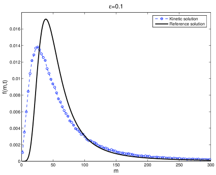
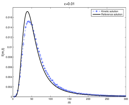
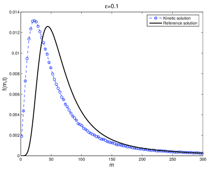
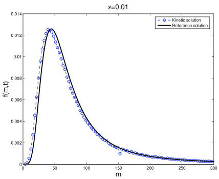
The test cases considered has been proposed in [31]. We start from an initial conditions where no mutants are present $f_{0}(m)=\delta(0)$ and $N_{0}=1$. The parameters are $\mu=10^{-7}$, $\alpha-\mu=3$ and the final computation time is $t=6.7$. To reduce fluctuations the total number of simulation samples is $5\times 10^{5}$. First we consider the Luria-Delbrück case for $\beta=2.5$ and then the Lea-Coulson case for $\beta=2.8$.

In Figure 2, we report the solution obtained simulating the kinetic model (7) for different values of the scaling parameter $\varepsilon$. The results show the convergence of the mutant distribution prescribed by model towards the classical Luria-Delbrück solution obtained using Lemma 2 in [31].

Similarly we report in Figure 3 the solution of the kinetic model (26) for different values of the scaling parameter $\varepsilon$. As expected convergence of the mutant distribution towards the Lea-Coulson solution, computed using Lemma 2 together with numerical quadrature as in [31], is observed.

Figure 2: Luria-Delbrück setting. Distribution of mutant cells at $t=6.7$ with $\beta=2.5$ for $\epsilon=0.1$ (top) and $\epsilon=0.01$ (bottom) in the kinetic model (7). The reference solution is computed using Lemma 2 in [31].

Figure 3: Lea-Coulson setting. Distribution of mutant cells at $t=6.7$ with $\beta=2.8$ for $\epsilon=0.1$ (top) and $\epsilon=0.01$ (bottom) in the kinetic model (26). The reference solution is computed using Lemma 2 in [31] and numerical quadrature.

5 Conclusions

We have derived kinetic and mean field equations corresponding to two most famous mathematical formulations of the Luria-Delbrück experiment. First we discussed the original Luria-Delbrück formulation and have shown that under a suitable mean field scaling the master equation yields a generalized Fokker-Planck equation having the Luria-Delbrück distribution as solution. Next we extended our approach to the Lea-Coulson case and derived the corresponding kinetic model and asymptotic generalized Fokker-Planck limit. Following the theoretical analysis we presented results of numerical experiments conducted using a Monte Carlo method. We have shown a computational evidence of convergence of our models towards the classical formulations.

Beside the mathematical aspects of the problem, the interest in the continuous modeling of the mutation process presented here is twofold. On the one hand, the models provide a new environment for the development of numerical methods to compute mutant distribution, and, on the other hand, they represent a first step towards the development of more realistic mean field models where the distribution function depends also on the physical location of the mutant cells.

References

- [1] W.P. Angerer, An explicit representation of the Luria Delbru ck distribution, J. Math. Biol. 42 (2001) 145.
- [2] P. Armitage, The statistical theory of bacterial populations subject to mutation, J. Royal Statist. Soc. B 14 (1952) 1.
- [3] M.S. Bartlett, An Introduction to Stochastic Processes, 3rd edition, Cambridge, London, (1978).
- [4] N. Bellomo, Modeling complex living systems: a kinetic theory and stochastic game approach, Birkhauser, (2008).
- [5] N. Bellomo, M. Delitala From the mathematical kinetic, and stochastic game theory to modelling mutations, onset, progression and immune competition of cancer cells, Physics of Life Reviews 5 (2008) 183 -206.
- [6] C. Cercignani, The Boltzmann equation and its applications, Springer, (1988).
- [7] S. Cordier, L. Pareschi, G. Toscani, On a kinetic model for a simple market economy. J. Stat. Phys., 120, (2005), 253 -277.
- [8] S. A. Frank, Dynamics of Cancer: Incidence, Inheritance, and Evolution. Princeton Series in Evolutionary Biology, Princeton University Press, (2007).
- [9] S. A. Frank, Somatic mosaicism and cancer: inference based on a conditional Luria-Delbrück distribution. Journal of Theoretical Biology, 223, (2003), 405 -412.
- [10] F. Grizzi, M. Chiriva-Internati, Cancer: looking for simplicity and finding complexity. Cancer Cell International, 6(4), (2006).
- [11] H. Hatzikirou, L. Brusch, C. Schaller, M. Simon, A. Deutsch, Prediction of traveling front behavior in a lattice-gas cellular automaton model for tumor invasion. Comput. Math. Appl. 59 (2010), no. 7, 2326–2339.
- [12] M.E. Jones, S.M. Thomas, A. Rogers, Luria Delbrück fluctuation experiments: design and analysis, Genetics 136 (1994) 1209.
- [13] A.W. Kemp, Comments on the Luria-Delbrück distribution. J. Appl. Prob. 31, (1994) 822–828.
- [14] D.G. Kendall, Birth-and-death process and the theory of carcinogenesis, Biometrika 47 (1960) 13.
- [15] T.B. Kepler, M. Oprea, Improved inference of mutation rates. I. An integral representation for the Luria-Delbrück distribution, Theor. Pop. Biol. 59, (2001) 41–48.
- [16] T.B. Kepler, M. Oprea, Improved inference of mutation rates. II. Generalization of the Luria-Delbrück distribution, Theor. Pop. Biol. 59, (2001) 49–59.
- [17] D.E. Knuth, Seminumerical Algorithms. The Art of Computer Programming, Volume 2, Addison Wesley, (1969).
- [18] D.E. Lea, C.A. Coulson, The distribution of the numbers of mutants in bacterial populations, J. Genetics 49 (1949) 264.
- [19] S.E. Luria, M. Delbrück, Mutations of bacteria from virus sensitivity to virus resistance, Genetics 28 (1943) 491.
- [20] B. Mandelbrot, A population birth-and-mutation process I: Explicit distributions for the number of mutants in an old culture of bacteria, J. Appl. Prob. 11 (1974) 437.
- [21] G. Marsaglia, The incomplete function as a continuous Poisson distribution, Computers & Mathematics with Applications, 12, (1986), 1187–1190.
- [22] J. Moreira, A. Deutsch, Cellular automaton models of tumor development: a critical review. Adv. Complex Syst. 5 (2002), no. 2-3, 247–267.
- [23] G. Naldi, L. Pareschi, G. Toscani, Mathematical modelling of collective behavior in socio-economic and life sciences, Birkhauser, (2010).
- [24] L. Natarajan, C. C. Berry, C. Gasche, Estimation of spontaneous mutation rates, Biometrics, 59, (2003), 555–561.
- [25] L. Pareschi, G. Russo, An introduction to Monte Carlo methods for the Boltzmann equation, ESAIM Proceedings, 10, (2001), 35–75. (Free access article at http://www.esaim-proc.org/articles/proc/pdf/2001/01/cemracs.pdf)
- [26] L. Pareschi, G. Toscani, Self-similarity and power-like tails in nonconservative kinetic models, J.Stat. Phys., 124, (2006), 747–779.
- [27] H. Risken, The Fokker-Planck equation: methods of solution and applications, Springer, (1996).
- [28] H. Risken, H.D. Vollmer, On solutions of truncated Kramers-Moyal expansions; continuum approximations to the Poisson process, Zeitschrift für Physik B Condensed Matter 66, (1987) 257–262.
- [29] V. Stohny, Symmetry Properties and Exact Solutions of the Fokker-Planck Equation, Nonlin. Math. Phys., 4, 1 2, (1997) 132- 136.
- [30] C. Villani, On a new class of weak solutions to the spatially homogeneous Boltzmann and Landau equations, Arch. Rational Mech. Anal. 143, (1998), 273–307.
- [31] Q. Zheng, Progress of a half century in the study of the Luria-Delbrück distribution, Math. Biosci. 162 (1999) 1-32.
- [32] Q. Zheng, New algorithms for Luria Delbrück fluctuation analysis, Math. Biosci. 196 (2005) 198.
- [33] Q. Zheng, On Haldane’s formulation of Luria and Delbrück’s mutation model, Math. Biosci. 209 (2007) 500 513.