Critical temperature of a Rashba spin-orbit coupled Bose gas in harmonic traps

Abstract

We investigate theoretically Bose-Einstein condensation of an ideal, trapped Bose gas in the presence of Rashba spin-orbit coupling. Analytic results for the critical temperature and condensate fraction are derived, based on a semi-classical approximation to the single-particle energy spectrum and density of states, and are compared with exact results obtained by explicitly summing discrete energy levels for small number of particles. We find a significant decrease of the critical temperature and of the condensate fraction due to a finite spin-orbit coupling. For large coupling strength and finite number of particles $N$, the critical temperature scales as $N^{2/5}$ and $N^{2/3}$ in three and two dimensions, respectively, contrasted to the predictions of $N^{1/3}$ and $N^{1/2}$ in the absence of spin-orbit coupling. Finite size corrections in three dimensions are also discussed.

I Introduction

The recent experiment on spin-orbit (SO) coupled spinor Bose gases of ⁸⁷Rb atoms Lin2011 has stimulated great interest in the theoretical study of SO physics in both Bose-Einstein condensation (BEC) and fermionic superfluidity. It is well-known that the SO coupling leads to many interesting phenomena in condensed matter physics. A typical example is the recently discovered topological insulators or quantum spin Hall states Qi2010 ; Hasan2010 . In degenerate atomic gases, due to unprecedented controllability in the interatomic interaction, geometry and purity Dalfovo1999 ; Bloch2008 , the SO coupling may bring even more intriguing states of matter Zhai2011 ; Stanescu2008 ; Larson2009 ; Wang2010 ; Wu2011 ; Ho2011 ; Xu2011 ; Hu2011a ; Sinha2011 ; Barnett2011 ; Zhu2011a ; Deng2011 ; Vyasanakere2011 ; Iskin2011 ; Zhu2011b ; Yu2011 ; Hu2011b ; Gong2011 ; Liu2011 .

For a SO coupled BEC, non-trivial structures, such as the density-stripe state Wang2010 ; Ho2011 , half-quantum vortex state Wu2011 and lattice state Hu2011a ; Sinha2011 , are predicted. For an atomic Fermi gas near Feshbach resonances, new two-fermion bound states with anisotropic mass are formed even at a negative $s$-wave scattering length Vyasanakere2011 ; Yu2011 ; Hu2011b , leading to the prospect of anisotropic superfluidity with mixed $s$- and $p$-wave components Hu2011b . By imposing an external Zeeman field, novel topological superfluid supporting zero-energy Majorana modes may also emerge Zhu2011b ; Gong2011 ; Liu2011 . To observe these new states of matter, it is necessarily to cool the temperature below a threshold, which may depend critically on the SO coupling. The purpose of this work is to determine the critical temperature of trapped atomic Bose gases with Rashba type SO coupling. We focus on an ideal, non-interacting Bose gas, since the critical temperature is less affected by weak interatomic interactions Giorgini1996 .

Theoretically, the critical temperature of a homogeneous Bose gas is greatly suppressed by the Rashba SO coupling, as the low-energy density of states (DOS) is dramatically modified Zhai2011 ; Vyasanakere2011 . In three dimensions (3D) without Rashba SO coupling, the low-energy DOS $\rho(E)$ vanishes as $\sqrt{E}$. As a result, the number of total particles occupied at finite energy levels, given by $N(T)=\int_{0}^{\infty}dE\rho(E)/(e^{E/k_{B}T}-1)$, saturates at finite temperature $T$ Dalfovo1999 . This leads to the well-known macroscopic occupation of the ground state, i.e., the formation of a BEC. In the presence of Rashba SO coupling, however, the low-energy DOS becomes a constant (see Appendix A) Zhai2011 ; Vyasanakere2011 , reminiscent of a two-dimensional (2D) system. The thermal occupation $N(T)$ can be logarithmically divergent. The critical temperature is therefore precisely zero, ruling out the possibility of BEC at any finite temperatures Dalfovo1999 .

In this paper, we show that in the presence of a harmonic trap the Rashba SO coupling does not destroy the BEC at finite temperatures, as the thermal occupation $N(T)$ remains finite. Actually, the critical temperature is not affected by the Rashba SO coupling in the thermodynamic limit where the number of particles $N$ becomes infinitely large. This is because the occupation of low-energy states, modified by the SO coupling, becomes negligible as $N\rightarrow\infty$. However, in the experimentally relevant situation in which numbers of particles range from a few thousand to a few million, we find a significant decrease of the critical temperature and of the condensate fraction. In particular, at a sufficiently large Rashba SO coupling strength, the critical temperature scales like $N^{2/5}$ and $N^{2/3}$ in three and two dimensions, respectively, in sharp contrast to the scaling of $N^{1/3}$ and $N^{1/2}$ without SO coupling Dalfovo1999 ; Ketterle1996 ; Haugerud1997 ; Balaz2010 . We derive these results either by summing discrete energy levels for small number of particles or by using a continuous DOS under the semi-classical assumption that the level spacing is negligible compared to the temperature. The former approach also enables the investigation of finite-size correction to the critical temperature.

The paper is structured as follows. In the next section (Sec. II), we introduce the theoretical model for Rashba spin-orbit coupled ideal Bose gases in harmonic traps and solve the single-particle energy spectrum. In Sec. III, we present the 2D and 3D DOS with or without the continuous spectrum approximation. The critical temperature and condensate fraction are then calculated in Sec. IV for both 2D and 3D cases. Next, the finite size effect in 3D is discussed in Sec. V. Finally, Sec. VI is devoted to conclusions. The calculation of the DOS of a homogeneous 3D Rashba SO coupled system is given in the Appendix A.

II Model Hamiltonian and single-particle energy spectrum

We consider a two-component (spin-1/2) Bose gas in 2D or 3D harmonic traps, $V_{2D}(r_{\perp})=M\omega_{\perp}^{2}(x^{2}+y^{2})/2\equiv M\omega_{\perp}^{2}r_{\perp}^{2}/2$ or $V_{3D}(r_{\perp},z)=M(\omega_{\perp}^{2}r_{\perp}^{2}+\omega_{z}^{2}z^{2})/2$, with a Rashba SO coupling ${\cal V}_{SO}=-i\lambda_{R}(\hat{\sigma}_{x}\partial_{y}-\hat{\sigma}_{y}\partial_{x})$ in the $x-y$ plane, where $\lambda_{R}$ is the Rashba SO coupling strength and $\hat{\sigma}_{x}$, $\hat{\sigma}_{y}$, and $\hat{\sigma}_{z}$ are the $2\times 2$ Pauli matrices for pseudo-spin. The model Hamiltonian for single-particle is described by,

$${\cal H}_{S}=\left[\begin{array}[]{cc}-\hbar^{2}\nabla^{2}/2M+V_{T}&-i\lambda_{R}(\partial_{y}+i\partial_{x})\\ -i\lambda_{R}(\partial_{y}-i\partial_{x})&-\hbar^{2}\nabla^{2}/2M+V_{T}\end{array}\right]$$ (1)

where the trapping potential $V_{T}({\bf r}_{\perp})=V_{2D}(r_{\perp})$ in 2D and $V_{T}({\bf r})=V_{3D}(r_{\perp},z)$ in 3D harmonic traps. The characteristic length scales of harmonic traps in the $x-y$ plane and $z$-direction are given by, $a_{\perp}=\sqrt{\hbar/(M\omega_{\perp})}$ and $a_{z}=\sqrt{\hbar/(M\omega_{z})}$, respectively. For the SO coupling, we take a dimensionless coupling strength $\lambda_{SO}\equiv\lambda_{R}Ma_{\perp}/\hbar^{2}$.

In the 2D case, it is convenient to use polar coordinates ${\bf r}_{\perp}=(r_{\perp},\varphi)$, in which $-i(\partial_{y}\pm i\partial_{x})=e^{\mp i\varphi}[\pm\partial/\partial r_{\perp}-(i/r_{\perp})\partial/\partial\varphi]$. As the harmonic potential is isotropic, the single-particle wave-function has a well-defined azimuthal angular momentum $l_{z}=m$ and takes the form,

$$\phi_{m}({\bf r}_{\perp})=\left[\begin{array}[]{c}\phi_{\uparrow}(r_{\perp})\\ \phi_{\downarrow}(r_{\perp})e^{i\varphi}\end{array}\right]\frac{e^{im\varphi}}{\sqrt{2\pi}},$$ (2)

which preserves the total angular momentum $j_{z}=l_{z}+s_{z}=m+1/2$. The Schrödinger equation for $\phi_{\uparrow}(r_{\perp})$ and $\phi_{\downarrow}(r_{\perp})$ therefore becomes,

$$\left[\begin{array}[]{cc}{\cal H}_{m}&\lambda_{R}\left[\partial/\partial r_{\perp}+\left(m+1\right)/r_{\perp}\right]\\ \lambda_{R}\left(-\partial/\partial r_{\perp}+m/r_{\perp}\right)&{\cal H}_{m+1}\end{array}\right]\left[\begin{array}[]{c}\phi_{\uparrow}\\ \phi_{\downarrow}\end{array}\right]=E_{nm}\left[\begin{array}[]{c}\phi_{\uparrow}\\ \phi_{\downarrow}\end{array}\right],$$ (3)

where ${\cal H}_{m}\equiv-[\hbar^{2}/(2M)][d/dr_{\perp}{}^{2}+(1/r_{\perp})d/dr_{\perp}-m^{2}/r_{\perp}{}^{2}]+M\omega_{\perp}^{2}r_{\perp}{}^{2}/2$ is the 2D harmonic oscillator. We have denoted the energy level as $E_{nm}$, with $n=(0,1,2...)$ being the good quantum number in the transverse (radial) direction. Each energy level is two-fold degenerate, as a result of the time-reversal symmetry satisfied by the single-particle model Hamiltonian (Kramer’s degeneracy). Any state $\phi({\bf r}_{\perp})=[\phi_{\uparrow}({\bf r}_{\perp}),\phi_{\downarrow}({\bf r}_{\perp})]^{T}$ is degenerate with its time-reversal partner ${\cal T}\phi({\bf r}_{\perp})\equiv(i\sigma_{y}{\cal C})\phi({\bf r}_{\perp})=$ $[\phi_{\downarrow}^{*}({\bf r}_{\perp}),-\phi_{\uparrow}^{*}({\bf r}_{\perp})]^{T}$, where ${\cal C}$ is the complex conjugate operator. Therefore, we may restrict the quantum number $m$ to be non-negative integers, as a state with negative $m$ can always be treated as the time-reversal partner of a state with $m\geq 0$. To solve numerically the single-particle spectrum, we expand the wave-function using the basis of 2D harmonic oscillator,

$$\phi_{\uparrow}(r_{\perp}) = \sum_{k=0}^{\infty}A_{\uparrow k}R_{km}\left(r_{\perp}\right),$$ (4)

$$\phi_{\downarrow}(r_{\perp}) = \sum_{k=0}^{\infty}A_{\downarrow k}R_{km+1}\left(r_{\perp}\right),$$ (5)

where

$$R_{km}=\frac{1}{a_{\perp}}\left[\frac{2k!}{\left(k+\left|m\right|\right)!}\right]^{1/2}\left(\frac{r_{\perp}}{a_{\perp}}\right)^{\left|m\right|}e^{-\frac{r_{\perp}^{2}}{2a_{\perp}^{2}}}{\cal L}_{k}^{\left|m\right|}(\frac{r_{\perp}^{2}}{a_{\perp}^{2}})$$ (6)

is the radial wave-function of ${\cal H}_{m}$ with energy $(2k+\left|m\right|+1)\hbar\omega_{\perp}$ and ${\cal L}_{k}^{\left|m\right|}$ is the associated Legendre polynomial. This leads to the following secular equation,

$$\left[\begin{array}[]{cc}{\cal H}_{m}&{\cal M}^{T}\\ {\cal M}&{\cal H}_{m+1}\end{array}\right]\left[\begin{array}[]{c}A_{\uparrow}\\ A_{\downarrow}\end{array}\right]=E_{nm}\left[\begin{array}[]{c}A_{\uparrow}\\ A_{\downarrow}\end{array}\right],$$ (7)

where the vectors $A_{\uparrow}$ and $A_{\downarrow}$ denote collectively the expanding coefficients $\{A_{\uparrow k}\}$ and $\{A_{\downarrow k}\}$, and the elements of matrices ($m\geq 0$) are given by,

$$\left({\cal H}_{m}\right)_{kk^{\prime}} = \left(2k+m+1\right)\delta_{kk^{\prime}}\hbar\omega_{\perp},$$ (8)

$${\cal M}_{kk^{\prime}} = \lambda_{SO}\left(\sqrt{k^{\prime}+m+1}\delta_{kk^{\prime}}+\sqrt{k^{\prime}}\delta_{kk^{\prime}-1}\right)\hbar\omega_{\perp}.$$ (9)

Diagonalization of the secular matrix Eq. (7) leads to the single-particle spectrum and single-particle wave-functions. In numerical calculations, it is necessary to truncate the radial quantum number $k$ of the 2D harmonic oscillator, by restricting $k<k_{\max}$. For $\lambda_{SO}\leq 20$, we find that $k_{\max}=256$ is already sufficiently large to have an accurate energy spectrum. With this cut-off, the dimension of the secular matrix in Eq. (7) is $2k_{\max}=512$.

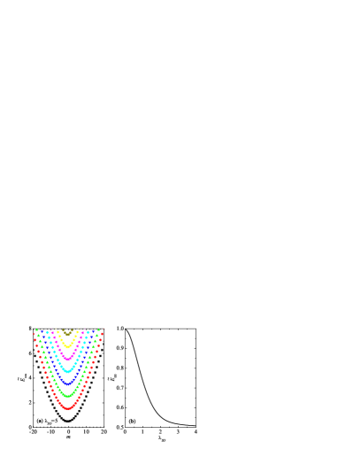
Figure 1: (color online). (a) Single-particle energy spectrum $\tilde{E}_{nm}=E_{nm}+(\lambda_{SO}^{2}/2)\hbar\omega_{\perp}$ at $\lambda_{SO}=5$, measured in reference to the semi-classical zero-point energy $-(\lambda_{SO}^{2}/2)\hbar\omega_{\perp}$. (b) Ground state single-particle energy, $\tilde{E}_{00}=E_{00}+(\lambda_{SO}^{2}/2)\hbar\omega_{\perp}$, as a function of the dimensionless Rashba SO coupling constant. The energy is plotted in units of $\hbar\omega_{\perp}$.

In Fig. 1a, we present the single-particle energy spectrum at $\lambda_{SO}=5$. The ground state single-particle energy is plotted in Fig. 1b as a function of the dimensionless SO coupling constant. In reference to the semi-classical zero-point energy $E_{0}^{sc}\equiv-(\lambda_{SO}^{2}/2)\hbar\omega_{\perp}$, the ground state energy decrease from $\hbar\omega_{\perp}$ to $\hbar\omega_{\perp}/2$, when the Rashba SO coupling strength $\lambda_{SO}$ becomes sufficiently large. In that limit (i.e., $\lambda_{SO}>5$), the low-lying energy spectrum becomes fairly flat, with a dispersion that is well approximated by Hu2011a ; Sinha2011 ,

$$E_{nm}\simeq\left[-\frac{\lambda_{SO}^{2}}{2}+(n+\frac{1}{2})+\frac{m\left(m+1\right)}{2\lambda_{SO}^{2}}\right]\hbar\omega_{\perp}.$$ (10)

In 3D, because the motions in $xy$-plane and $z$-direction are decoupled, the single-particle energy spectrum is given by,

$$E_{nmn_{z}}=E_{nm}+\left(n_{z}+\frac{1}{2}\right)\hbar\omega_{z},$$ (11)

where $n_{z}=0,1,2...$ is a good quantum number for the axial motion.

At finite temperature $T$, the total number of particles is given, in the grand-canonical ensembles, by the sum

$$N=\sum_{n,m=0}^{\infty}\frac{2}{\exp\left[\left(E_{nm}-\mu\right)/k_{B}T\right]-1}$$ (12)

in 2D and by the sum

$$N=\sum_{n,m,n_{z}=0}^{\infty}\frac{2}{\exp\left[\left(E_{nmn_{z}}-\mu\right)/k_{B}T\right]-1}$$ (13)

in 3D, where $\mu$ is the chemical potential and the factor of $2$ arises from the Kramer’s degeneracy. The sum can be rewritten as an integral over the energy, in the unified form,

$$N=\int_{-\infty}^{+\infty}dE\frac{\rho\left(E\right)}{\exp\left[\left(E-\mu\right)/k_{B}T\right]-1},$$ (14)

with the DOS $\rho\left(E\right)$ given by

$$\rho_{2D}\left(E\right)=2\sum_{n,m=0}^{\infty}\delta\left(E-E_{nm}\right)$$ (15)

and

$$\rho_{2D}\left(E\right)=2\sum_{n,m,n_{z}=0}^{\infty}\delta\left(E-E_{nmn_{z}}\right),$$ (16)

in 2D and 3D, respectively.

For given small numbers of particles $N$, we can calculate the low-lying energy levels and then sum explicitly the number equations, Eqs. (12) and (13). Once the chemical potential is determined at a given temperature $T$, we calculate the occupation of the ground state,

$$N_{0}=\frac{2}{\exp\left[\left(E_{0}-\mu\right)/k_{B}T\right]-1},$$ (17)

where the single-particle ground state energy $E_{0}=E_{00}$ in 2D and $E_{0}=E_{00}+\hbar\omega_{z}/2$ in 3D. The BEC transition temperature $T_{c}$ can be determined from $d^{2}N_{0}/dT^{2}$, which exhibits a maximum at $T_{c}$ Bergeman2000 .

III Semi-classical density of states

For large numbers of particles, it is useful to consider a semi-classical approximation by using continuous energy spectrum Dalfovo1999 . The level spacing, typical of $\hbar\omega_{\perp}$ or $\hbar\omega_{z}$, is assumed to be negligibly small, compared with the thermal energy $k_{B}T$. Thus, the relevant excitation energies, contributing to the sum in Eqs. (12) and (13), are much larger than the level spacing. The accuracy of the semi-classical approximation can be tested a posteriori by comparing the semi-classical result with the numerical discrete summation.

III.1 2D density of states

In 2D, the semi-classical DOS can be written as,

$$\rho_{2D}^{sc}\left(E\right)=\sum_{s=\pm}\int\frac{d{\bf r}_{\perp}d{\bf k}_{\perp}}{\left(2\pi\right)^{2}}\delta\left[E_{{\bf k}s}({\bf r}_{\perp})-E\right],$$ (18)

where $E_{{\bf k}s}({\bf r}_{\perp})=\hbar^{2}k_{\perp}^{2}/(2M)+s\lambda_{R}k_{\perp}+M\omega_{\perp}^{2}r_{\perp}^{2}/2$ is the semi-classical energy in phase space (${\bf r}_{\perp},{\bf k}_{\perp}$). Because of the Rashba SO coupling, the semi-classical energy splits into two helicity branches as indicated by $s=\pm$ (see Appendix A). By integrating out the spatial degree of freedom, we obtain that,

$$\hbar\omega_{\perp}\rho_{2D}^{sc}\left(E\right)=\sum_{s=\pm}\int\limits_{0}^{\infty}\tilde{k}_{\perp}d\tilde{k}_{\perp}\Theta\left[\frac{\tilde{E}}{\hbar\omega_{\perp}}-\frac{\left(\tilde{k}_{\perp}+s\lambda_{SO}\right)^{2}}{2}\right],$$ (19)

where $\tilde{k}_{\perp}\equiv k_{\perp}a_{\perp}$ is the dimensionless wave-vector, $\tilde{E}\equiv E+(\lambda_{SO}^{2}/2)\hbar\omega_{\perp}$ is the energy measured in reference to the semi-classical zero-point energy $E_{0}^{sc}\equiv-(\lambda_{SO}^{2}/2)\hbar\omega_{\perp}$, and $\Theta(\cdot)$ is the Heaviside step function. The integration over the wave-vector can be calculated explicitly as well. We finally arrive at,

$$\hbar\omega_{\perp}\rho_{2D}^{sc}\left(E\right)=\left\{\begin{array}[]{ll}0,&\left(E<E_{0}^{sc}\right);\\ 2\lambda_{SO}\left[2E/\left(\hbar\omega_{\perp}\right)+\lambda_{SO}^{2}\right]^{1/2},&(E_{0}^{sc}\leq E<0);\\ 2E/\left(\hbar\omega_{\perp}\right)+2\lambda_{SO}^{2},&(E\geq 0).\end{array}\right.$$ (20)

In the absence of Rashba SO coupling ($\lambda_{SO}=0$), we recover the usual expression for the 2D DOS in harmonic traps, $\rho_{2D}^{sc}\left(E\right)=2E/(\hbar\omega_{\perp})^{2}\Theta(E)$, for a two-component system Dalfovo1999 .

III.2 3D density of states

Likewise, we calculate the semi-classical DOS in 3D, which is given by,

$$\rho_{3D}^{sc}\left(E\right)=\sum_{s=\pm}\int\frac{d{\bf r}d{\bf k}}{\left(2\pi\right)^{3}}\delta\left[E_{{\bf k}s}({\bf r})-E\right],$$ (21)

where the semi-classical energy now takes the form $E_{{\bf k}s}({\bf r})=\hbar^{2}k_{\perp}^{2}/(2M)+s\lambda_{R}k_{\perp}+\hbar^{2}k_{z}^{2}/(2M)+M(\omega_{\perp}^{2}r_{\perp}^{2}+\omega_{z}^{2}z^{2})/2$. The integration over ${\bf r}$ and $k_{z}$ can be done by introducing a new variable $t^{2}=\hbar^{2}k_{z}^{2}/(2M)+M(\omega_{\perp}^{2}r_{\perp}^{2}+\omega_{z}^{2}z^{2})/2$ and by converting the variables of integration $d{\bf r}d{\bf k}$ to $d{\bf t}d{\bf k}_{\perp}$. This leads to,

$$\hbar\omega_{z}\rho_{3D}^{sc}\left(E\right)=\sum_{s=\pm}\int\limits_{0}^{\infty}\tilde{k}_{\perp}d\tilde{k}_{\perp}\left[\frac{\tilde{E}}{\hbar\omega_{\perp}}-\frac{\left(\tilde{k}_{\perp}+s\lambda_{SO}\right)^{2}}{2}\right]\Theta\left[\frac{\tilde{E}}{\hbar\omega_{\perp}}-\frac{\left(\tilde{k}_{\perp}+s\lambda_{SO}\right)^{2}}{2}\right].$$ (22)

By explicitly integrating out $\tilde{k}_{\perp}$, we obtain,

$$\hbar\omega_{z}\rho_{3D}^{sc}\left(E\right)=\left\{\begin{array}[]{ll}0,&\left(E<E_{0}^{sc}\right);\\ \left(2\lambda_{SO}/3\right)\left[2E/\left(\hbar\omega_{\perp}\right)+\lambda_{SO}^{2}\right]^{3/2},&(E_{0}^{sc}\leq E<0);\\ \left[E/\left(\hbar\omega_{\perp}\right)+\lambda_{SO}^{2}\right]^{2}-\lambda_{SO}^{4}/3,&(E\geq 0).\end{array}\right.$$ (23)

In the absence of Rashba SO coupling, we recover the expression $\rho_{3D}^{sc}\left(E\right)=E^{2}/\left(\hbar^{3}\omega_{\perp}^{2}\omega_{z}\right)\Theta(E)$ for 3D harmonic traps Dalfovo1999 .

It is easy to check that the 2D and 3D DOS is related by

$$\hbar\omega_{z}\frac{d\rho_{3D}^{sc}\left(E\right)}{dE}=\rho_{2D}^{sc}\left(E\right).$$ (24)

This is due to the decoupled motion in the $x-y$ plane and $z$ direction, which leads to the observation that the 3D energy spectrum may alternatively be viewed as a collection of 2D spectra with regular spacing $\hbar\omega_{z}$.

III.3 Test of the semi-classical DOS

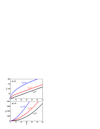
Figure 2: (color online). The semi-classical density of states in 2D (a) and 3D (b), in units of $1/(\hbar\omega_{\perp})$ and $1/(\hbar\omega_{z})$ respectively, are shown as a function of $\tilde{E}=E+(\lambda_{SO}^{2}/2)\hbar\omega_{\perp}$ at different Rashba SO couplings (solid lines). The energy $\tilde{E}$ is in units of $\hbar\omega_{\perp}$. For comparison, the symbols plot the results obtained by the numerical summation, see, Eqs. (15) and (16). The simulation of the delta-function is described in the text.

In Fig. 2, we compare the semi-classical 2D and 3D DOS with these obtained by summing over the discrete single-particle energy spectrum using Eqs. (15) and (16). In the numerical summation, we simulate the $\delta$-function $\delta(x)$ by a Lorentzen line shape with broadening $\Gamma$, $f_{\delta}(x;\Gamma)=(\Gamma/\pi)/(x^{2}+\Gamma^{2})$. Roughly, the resulting DOS depends linearly on $\Gamma$ at $\Gamma\sim\hbar\omega_{\perp}$. Therefore, we use

$$\delta(x)=2f_{\delta}(x;\Gamma=\hbar\omega_{\perp})-f_{\delta}(x;\Gamma=2\hbar\omega_{\perp}),$$ (25)

as an extrapolation to the zero-broadening limit ($\Gamma=0$). We find that the semi-classical expressions for DOS, Eqs. (19) and (22), works extremely well over a very broad range for energy. The most significant discrepancy occurs at the lowest energy level, $E\sim-(\lambda_{SO}^{2}/2)\hbar\omega_{\perp}$, as anticipated.

IV Critical temperature and condensate fraction

We are now ready to calculate the critical temperature and condensate fraction for large number of particles. With the semi-classical DOS $\rho^{sc}\left(E\right)$, the number of particles could be rewritten as Dalfovo1999 ,

$$N=N_{0}+\int_{E_{0}^{sc}}^{+\infty}dE\frac{\rho^{sc}\left(E\right)}{\exp\left[\left(E-\mu\right)/k_{B}T\right]-1},$$ (26)

where the ground state population $N_{0}$ is singled out and the finite sum over the excited states in Eqs. (12) and (13) is replaced by an integral. Accordingly, we have set the lower-bound of the integral to be the semi-classical zero-point energy $E_{0}^{sc}=-(\lambda_{SO}^{2}/2)\hbar\omega_{\perp}$. When BEC occurs, the chemical potential approaches to $E_{0}^{sc}$ from below Dalfovo1999 . The critical temperature $T_{c}$ is determined by the condition,

$$N=\int_{0}^{+\infty}d\tilde{E}\frac{\rho^{sc}\left(\tilde{E}+E_{0}^{sc}\right)}{\exp\left[\tilde{E}/k_{B}T_{c}\right]-1},$$ (27)

where $\tilde{E}\equiv E-E_{0}^{sc}$, and the condensate fraction at $T<T_{c}$ can be calculated by,

$$\frac{N_{0}}{N}=1-\frac{1}{N}\int_{0}^{+\infty}d\tilde{E}\frac{\rho^{sc}\left(\tilde{E}+E_{0}^{sc}\right)}{\exp\left[\tilde{E}/k_{B}T\right]-1}.$$ (28)

As we shall see, these equations can be conveniently solved by introducing $\epsilon=\tilde{E}/(k_{B}T)$ and

$$\alpha(T)=\lambda_{SO}\sqrt{\frac{\hbar\omega_{\perp}}{k_{B}T}}.$$ (29)

IV.1 2D

In 2D, the equations for the critical temperature and condensate fraction becomes,

$$N=\left(\frac{k_{B}T_{c}}{\hbar\omega_{\perp}}\right)^{2}{\cal I}_{2D}\left[\alpha\left(T_{c}\right)\right]$$ (30)

and

$$\frac{N_{0}}{N}=1-\left(\frac{T}{T_{c}}\right)^{2}\frac{{\cal I}_{2D}\left[\alpha\left(T\right)\right]}{{\cal I}_{2D}\left[\alpha\left(T_{c}\right)\right]},$$ (31)

respectively. Here the integral ${\cal I}_{2D}\left[\alpha\right]$ takes the form,

$${\cal I}_{2D}\left[\alpha\right]=\int_{0}^{+\infty}d\epsilon\frac{\tilde{\rho}_{2D}^{sc}\left(\epsilon;\alpha\right)}{e^{\epsilon}-1},$$ (32)

where the dimensionless DOS $\tilde{\rho}_{2D}^{sc}\left(\epsilon;\alpha\right)$ is given by,

$$\tilde{\rho}_{2D}^{sc}\left(\epsilon;\alpha\right)=\left\{\begin{array}[]{ll}0,&\left(\epsilon<0\right);\\ 2\alpha\sqrt{2\epsilon},&(0\leq\epsilon<\alpha^{2}/2);\\ 2\epsilon+\alpha^{2},&(\epsilon\geq\alpha^{2}/2).\end{array}\right.$$ (33)

Therefore,

$${\cal I}_{2D}\left[\alpha\right]=\sqrt{2\pi}\alpha\zeta\left(\frac{3}{2}\right)+\int\limits_{\alpha^{2}/2}^{+\infty}d\epsilon\frac{\left(\sqrt{2\epsilon}-\alpha\right)^{2}}{e^{\epsilon}-1}.$$ (34)

Here $\zeta(\cdot)$ is the Riemann $\zeta$ function. ${\cal I}_{2D}\left[\alpha\right]$ depends implicitly on the temperature through the dimensionless parameter $\alpha(T)$. It is clear from Eq. (29) that for a given SO coupling $\lambda_{SO}$, the dimensionless parameter $\alpha$ at the critical temperature $T_{c}$ always scales to zero in the thermodynamic limit $N\rightarrow\infty$. This is understandable as a finite SO interaction modifies only the low-lying energy states, whose occupation becomes negligible as $N\rightarrow\infty$.

In the absence of SO coupling, ${\cal I}_{2D}[\alpha=0]=2\zeta(2)=\pi^{2}/3$, we recover the standard results in 2D Dalfovo1999 ,

$$k_{B}T_{c}^{(0)}\left(\lambda_{SO}=0\right)=\frac{1}{\pi}\left(3N\right)^{1/2}\hbar\omega_{\perp}$$ (35)

and $N_{0}/N=1-(T/T_{c}^{(0)})^{2}$. Here, we use the superscript “$0$” to indicate the semi-classical result. For a large SO coupling, ${\cal I}_{2D}\left[\alpha\gg 1\right]=\sqrt{2\pi}\alpha\zeta\left(3/2\right)$, we find

$$k_{B}T_{c}^{(0)}\left(\lambda_{SO}\gg 1\right)=\frac{1}{\left(2\pi\right)^{1/3}}\left[\frac{N}{\lambda_{SO}\zeta\left(3/2\right)}\right]^{2/3}\hbar\omega_{\perp}$$ (36)

and $N_{0}/N=1-(T/T_{c}^{(0)})^{3/2}$. Thus, for a given number of particles, with increasing SO coupling the dependence of 2D critical temperature on the number of particles changes from $N^{1/2}$ to $N^{2/3}$. Using $\alpha\gg 1$, the strong-coupling limit is reached when

$$\lambda_{SO}\gg\left(2\pi\right)^{-1/8}\left[\frac{N}{\zeta\left(3/2\right)}\right]^{1/4}.$$ (37)

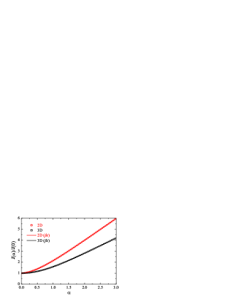
Figure 3: (color online). The integrals ${\cal I}_{2D}$ and ${\cal I}_{3D}$ as a function of the dimensionless parameter $\alpha=\lambda_{SO}[\hbar\omega_{\perp}/(k_{B}T)]^{1/2}$ (symbols). The solid lines show the empirical fit which agrees numerically within $0.5\%$ relative error (see the text for the empirical formalism).

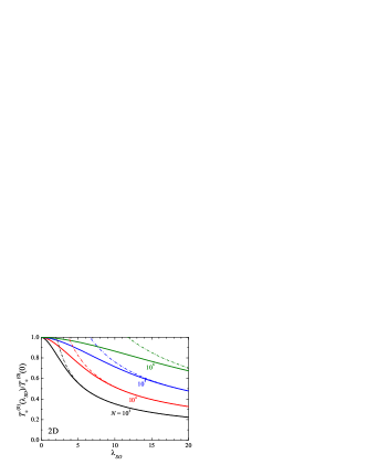
Figure 4: (color online). 2D critical temperature as a function of the SO coupling at different numbers of particles, as indicated. The dot-dashed lines show the limiting behavior at large SO coupling, Eq. (36).

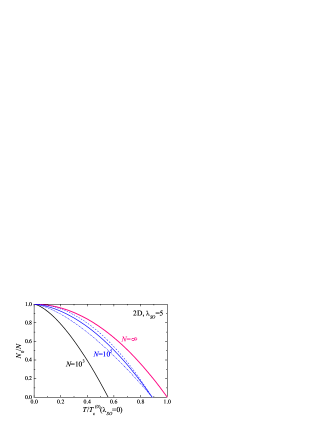
Figure 5: (color online). 2D condensate fraction at $\lambda_{SO}=5$ and at different numbers of particles. For the case of $N=10^{5}$, the dashed and dot-dashed lines show respectively the strong-coupling and zero-coupling result, $N_{0}/N=1-(T/T_{c}^{(0)})^{2}$ and $N_{0}/N=1-(T/T_{c}^{(0)})^{3/2}$.

In Fig. 3, we show ${\cal I}_{2D}\left[\alpha\right]$ as a function of the dimensionless parameter $\alpha$. Empirically, we find that ${\cal I}_{2D}\left[\alpha\right]\simeq\sqrt{2\pi}\alpha\zeta\left(3/2\right)+2\zeta(2)e^{-1.84\alpha-0.13\alpha^{2}}$, within $0.5\%$ relative error. Fig. 4 reports the critical temperature as a function of SO coupling at several numbers of particles (solid lines). It decreases significantly at moderate SO coupling ($\lambda_{SO}\sim 10$) and number of particles (i.e., $N\sim 10^{4}$). The strong-coupling results Eq. (36) have also been plotted using dot-dashed lines. Finally, in Fig. 5, we present the condensate fraction at $\lambda_{SO}=5$ and $N=10^{3}$, $10^{5}$, and $\infty$.

IV.2 3D

In 3D, similarly we obtain that

$$N\lambda=\left(\frac{k_{B}T_{c}}{\hbar\omega_{\perp}}\right)^{3}{\cal I}_{3D}\left[\alpha\left(T_{c}\right)\right]$$ (38)

and

$$\frac{N_{0}}{N}=1-\left(\frac{T}{T_{c}}\right)^{3}\frac{{\cal I}_{3D}\left[\alpha\left(T\right)\right]}{{\cal I}_{3D}\left[\alpha\left(T_{c}\right)\right]},$$ (39)

where $\lambda=\omega_{z}/\omega_{\perp}$ is the aspect ratio of the harmonic trap, the integral ${\cal I}_{3D}\left[\alpha\right]$ is given by,

$${\cal I}_{3D}\left[\alpha\right]=\int_{0}^{+\infty}d\epsilon\frac{\tilde{\rho}_{3D}^{sc}\left(\epsilon;\alpha\right)}{e^{\epsilon}-1},$$ (40)

and the dimensionless DOS $\tilde{\rho}_{3D}^{sc}\left(\epsilon;\alpha\right)$ is,

$$\tilde{\rho}_{3D}^{sc}\left(\epsilon;\alpha\right)=\left\{\begin{array}[]{ll}0,&\left(\epsilon<0\right);\\ (4\sqrt{2}\alpha/3)\epsilon^{3/2},&(0\leq\epsilon<\alpha^{2}/2);\\ \epsilon^{2}+\epsilon\alpha^{2}-\alpha^{4}/12,&(\epsilon\geq\alpha^{2}/2).\end{array}\right.$$ (41)

Explicitly, we find that

$${\cal I}_{3D}\left[\alpha\right]=\sqrt{2\pi}\alpha\zeta\left(\frac{5}{2}\right)+\int\limits_{\alpha^{2}/2}^{+\infty}d\epsilon\frac{h\left(\epsilon\right)}{e^{\epsilon}-1},$$ (42)

where $h\left(\epsilon\right)=\epsilon^{2}+\epsilon\alpha^{2}-\alpha^{4}/12-(4\sqrt{2}\alpha/3)\epsilon^{3/2}$. We plot ${\cal I}_{3D}\left[\alpha\right]$ in Fig. 3, together with an empirical fit, ${\cal I}_{3D}\left[\alpha\right]=\sqrt{2\pi}\alpha\zeta\left(5/2\right)+2\zeta(3)e^{-1.40\alpha-0.30\alpha^{2}}$.

At $\lambda_{SO}=0$ where ${\cal I}_{3D}[\alpha=0]=2\zeta(3)$, we obtain

$$k_{B}T_{c}^{(0)}\left(\lambda_{SO}=0\right)=\left[\frac{N\lambda}{2\zeta(3)}\right]^{1/3}\hbar\omega_{\perp}$$ (43)

and $N_{0}/N=1-(T/T_{c}^{(0)})^{3}$, recovering the well-known 3D result for a trapped spin-1/2 Bose gas Dalfovo1999 . In the limit of large SO coupling where ${\cal I}_{3D}\left[\alpha\gg 1\right]=\sqrt{2\pi}\alpha\zeta\left(5/2\right)$, we find instead

$$k_{B}T_{c}^{(0)}\left(\lambda_{SO}\gg 1\right)=\frac{1}{\left(2\pi\right)^{1/5}}\left[\frac{N\lambda}{\lambda_{SO}\zeta\left(5/2\right)}\right]^{2/5}\hbar\omega_{\perp}$$ (44)

and $N_{0}/N=1-(T/T_{c}^{(0)})^{5/2}$. Thus, for given $N$, with increasing SO coupling the power-law dependence of 3D critical temperature on number of particles changes from $N^{1/3}$ to $N^{2/5}$. We estimate that the strong-coupling result is applicable if

$$\lambda_{SO}\gg\left(2\pi\right)^{-1/12}\left[\frac{N\lambda}{\zeta\left(5/2\right)}\right]^{1/6}.$$ (45)

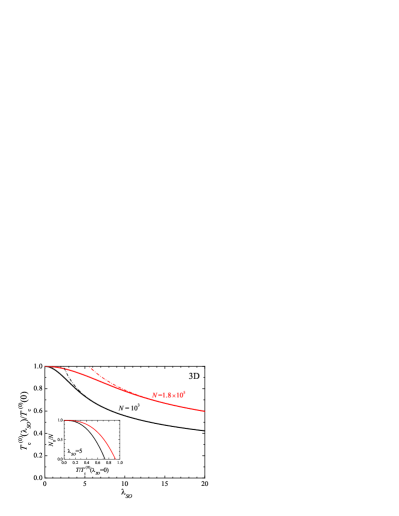
Figure 6: (color online). 3D critical temperature as a function of the SO coupling strength at $N=10^{3}$ and $N=1.8\times 10^{5}$. The aspect ratio of the harmonic trap is $\lambda=\omega_{z}/\omega_{\perp}=\sqrt{8}$. The dot-dashed lines show the critical temperature in the strong-coupling limit, Eq. (44). The inset reports the condensate fraction at $\lambda_{SO}=5$.

In Fig. 6, we report the effect of the SO coupling on 3D critical temperature. To make a connection with the NIST experiment Lin2011 , we have used a realistic aspect ratio of the trapping potential and number of particles, $\lambda=\sqrt{8}$ and $N=1.8\times 10^{5}$. We also consider the case with a small number of particles $N=10^{3}$. At the typical SO coupling strength $\lambda_{SO}\sim 10$ Lin2011 , the reduction of the critical temperature is about $20\%$, which is in reach of current experiments. The inset shows the condensate fraction at $\lambda_{SO}=5$.

V Finite size correction to $T_{c}$ in 3D

We now turn to consider the finite size correction to the semi-classical results, which arises from the discreteness of the single-particle energy spectrum Ketterle1996 ; Haugerud1997 . The semi-classical results are obtained using the semi-classical approximation for the excited states and setting the chemical potential to the semi-classical zero-point energy $E_{0}^{sc}$. To the leading order, the finite size correction can be included by still employing the semi-classical description for the excited states, while keeping the quantum value $\mu=E_{0}$ for the chemical potential at the transition Giorgini1996 . Here, $E_{0}>E_{0}^{sc}$ is the single-particle energy of the ground state. It is $E_{00}$ in 2D and $E_{00}+\hbar\omega_{z}/2$ in 3D; see, for example, Fig. (1b) for $E_{00}$ as a function of the SO coupling strength. The discreteness of the excited energy spectrum gives rise to higher-order finite size corrections. In the following, we focus on the finite size correction to the 3D critical temperature.

Using the quantum value $\mu=E_{0}$ for the chemical potential, the 3D critical temperature is determined by,

$$N = \int_{E_{0}}^{+\infty}dE\frac{\rho_{3D}^{sc}\left(E\right)}{\exp\left[\left(E-E_{0}\right)/k_{B}T_{c}\right]-1},$$ (46)

$$= \int_{0}^{+\infty}dE\frac{\rho_{3D}^{sc}\left(\tilde{E}+E_{0}^{sc}+\Delta E\right)}{\exp\left[\tilde{E}/k_{B}T_{c}\right]-1},$$ (47)

where in the second line we have introduced $\tilde{E}=E-E_{0}$ and $\Delta E=E_{0}-E_{0}^{sc}>0$. Compared with Eq. (27), the 3D DOS is slightly up-shifted by an amount $\Delta E$. As $\Delta E\sim\hbar\omega_{\perp}$ is the smallest energy scale, using Eq. (24) we may write $\rho_{3D}^{sc}(\tilde{E}+E_{0}^{sc}+\Delta E)\simeq\rho_{3D}^{sc}(\tilde{E}+E_{0}^{sc})+(\Delta E/\hbar\omega_{z})\rho_{2D}^{sc}(\tilde{E}+E_{0}^{sc})$. Therefore, using the integrals ${\cal I}_{2D}$ and ${\cal I}_{3D}$ the equation for the critical temperature is given by

$$N\lambda=\left(\frac{k_{B}T_{c}}{\hbar\omega_{\perp}}\right)^{3}\left[{\cal I}_{3D}\left[\alpha\left(T_{c}\right)\right]+\frac{\Delta E}{k_{B}T_{c}}{\cal I}_{2D}\left[\alpha\left(T_{c}\right)\right]\right].$$ (48)

In the absence of the SO coupling, ${\cal I}_{2D}=2\zeta(2)$, ${\cal I}_{3D}=2\zeta(3)$ and $\Delta E=\hbar\omega_{\perp}+\hbar\omega_{z}/2$, it is easy to verify that the transition temperature $T_{c}$ is given by the law,

$$\frac{T_{c}}{T_{c}^{0}}\simeq 1-\frac{\zeta(2)}{\left[2\zeta(3)\right]^{2/3}}N^{-1/3}\frac{\left(2\hbar\omega_{\perp}+\hbar\omega_{z}\right)/3}{\left(\omega_{\perp}^{2}\omega_{z}\right)^{1/3}},$$ (49)

which is known in the literature Giorgini1996 ; Ketterle1996 ; Haugerud1997 .

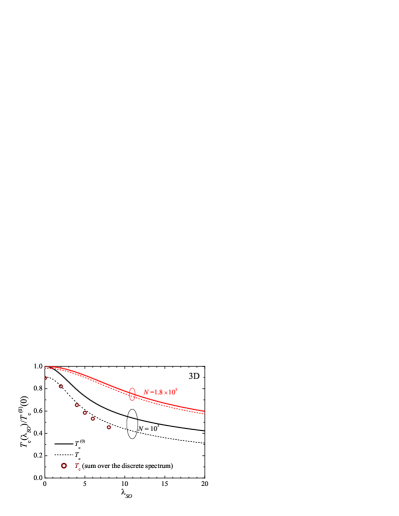
Figure 7: (color online). 3D transition temperature as a function of the SO coupling. The solid lines show the semi-classical predictions and the dashed line gives the results with inclusion of the leading finite size correction. The empty circles are calculated using the numerical summation for $N_{0}$ with discrete energy spectrum, i.e. Eq. (17). The critical temperature is then determined from the peak position of $d^{2}N_{0}/dT^{2}$ Bergeman2000 .

In Fig. 7, we report the 3D transition temperature with the leading finite size correction, as shown by dashed lines. We find a sizable correction at small number of particles (i.e., $N=10^{3}$). For the experimentally realistic number of particles, i.e., $N=1.8\times 10^{5}$, however, the correction becomes mild. As a benchmark to our analytic treatment for $T_{c}$, we also show by symbols the critical temperature for small number of particles, calculated by the discrete sum for the ground state population $N_{0}$, Eq. (17). At relatively small SO coupling (i.e., $\lambda_{SO}<5$), our analytic treatment works very well. However, for large SO coupling, the single-particle level splitting between the ground state and the first excited state becomes increasing small. We then may have to take into account the discreteness of the low-lying excited energy levels.

VI Conclusions

In summary, we have investigated the critical temperature and condensate fraction of a harmonically trapped ideal Bose gas in the presence of Rashba spin-orbit coupling, by using either the exact numerical summation for small number of particles or the analytic semi-classical approach for large number of particles. The leading finite size correction to the semi-classical approximation has also been considered. We have found pronounced effect of the Rashba SO coupling. For the experimentally realistic number of particles ($N\sim 10^{5}$) Lin2011 , the critical temperature is reduced by more than 20% in magnitude at a moderate SO coupling. This reduction is readily observable in current experiments. Moreover, in the limit of strong SO coupling, the critical temperature scales as $N^{2/5}$ and $N^{2/3}$ in three and two dimensions, respectively, which should be contrasted with the scaling law of $N^{1/3}$ and $N^{1/2}$ in the absence SO coupling. Our investigation of critical temperature can be easily extended to include a weak repulsive interaction, by using mean-field Hartree-Fock theory Giorgini1996 .

Appendix A Density of states of a 3D homogeneous SO coupled system

In free space, the single-particle Hamiltonian with Rashba SO coupling,

$${\cal H}_{S}=\left[\begin{array}[]{cc}-\hbar^{2}\nabla^{2}/2M&-i\lambda_{R}(\partial_{y}+i\partial_{x})\\ -i\lambda_{R}(\partial_{y}-i\partial_{x})&-\hbar^{2}\nabla^{2}/2M\end{array}\right],$$ (50)

has the dispersion,

$$E_{{\bf k}s}=\frac{\hbar^{2}k_{z}^{2}}{2M}+\frac{\hbar^{2}k_{\perp}^{2}}{2M}+s\lambda_{R}k_{\perp}.$$ (51)

Here $s=\pm$ denotes the two helicity branches. The DOS, given by $\rho(E)=(1/V)\sum_{{\bf k}}[\delta(E_{{\bf k}+}-E)+\delta(E_{{\bf k}-}-E)]$, can be calculated analytically. We find that,

$$\rho\left(E\right)=\frac{M^{2}\lambda_{R}}{\hbar^{4}}\left\{\begin{array}[]{ll}0,&\left(E<-E_{R}/2\right);\\ \pi/2,&(-E_{R}/2\leq E<0);\\ \sqrt{2E/E_{R}}+\left[\pi/2-\arctan\sqrt{2E/E_{R}}\right],&(E\geq 0).\end{array}\right.$$ (52)

where $E_{R}\equiv M\lambda_{R}^{2}/\hbar^{2}$ is the characteristic energy related to the SO coupling. This result was reported by Hui Zhai in Ref. Zhai2011 (see for example, their Fig. 2b). By introducing a Fermi wave-vector $k_{F}=(3\pi^{2}N/V)^{1/3}$, Fermi energy $E_{F}=\hbar^{2}k_{F}^{2}/(2M)$, and dimensionless SO coupling strength $\lambda_{eff}=M^{2}\lambda_{R}/(\hbar^{2}k_{F})$, the DOS can be written as,

$$\rho\left(E\right)=\frac{Mk_{F}}{\hbar^{2}}\left\{\begin{array}[]{ll}0,&\left(E<-\lambda_{eff}^{2}\right);\\ \lambda_{eff}\pi/2,&(-\lambda_{eff}^{2}\leq E<0);\\ \sqrt{E/E_{F}}+\lambda_{eff}\left[\pi/2-\arctan\sqrt{E/\left(\lambda_{eff}^{2}E_{F}\right)}\right],&(E\geq 0).\end{array}\right..$$ (53)

We show in Fig. 8 the DOS at different SO coupling strengths.

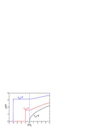
Figure 8: (color online). Density of states of a 3D homogeneous SO coupled system at several SO coupling strengths. The density of state is plotted in units of $Mk_{F}/\hbar^{2}$.

References

- (1) Y.-J. Lin, K. Jiménez-García, and I. B. Spielman, Nature (London) 471, 83 (2011).
- (2) X. L. Qi and S. C. Zhang, Physics Today 63, 33 (2010).
- (3) M. Z. Hasan and C. L. Kane, Rev. Mod. Phys. 82, 3045 (2010).
- (4) F Dalfovo, S. Giorgini, L. P. Pitaevskii, and S. Stringari, Rev. Mod. Phys. 71, 463 (1999).
- (5) I. Bloch, J. Dalibard, and W. Zwerger, Rev. Mod. Phys. 80, 885 (2008).
- (6) For a mini-reivew, see, H. Zhai, eprint arXiv:1110.6798.
- (7) T. D. Stanescu, B. Anderson, and V. Galitski, Phys. Rev. A 78, 023616 (2008).
- (8) J. Larson and E. Sjöqvist, Phys. Rev. A 79, 043627 (2009).
- (9) C. Wang, C. Gao, G.-M. Jian, and H. Zhai, Phys. Rev. Lett. 105, 160403 (2010).
- (10) C. Wu, I. Mondragon-Shem, and X.-F. Zhou, Chin. Phys. Lett. 28, 097102 (2011).
- (11) T.-L. Ho and S. Zhang, Phys. Rev. Lett. 107, 150403 (2011).
- (12) X. Q. Xu and J. H. Han, Phys. Rev. Lett. 107, 200401 (2011).
- (13) H. Hu, B. Ramachandhran, H. Pu, and X.-J. Liu, eprint arXiv:1108.4233; Phys. Rev. Lett. (in press 2011).
- (14) S. Sinha, R. Nath, and L. Santos, eprint arXiv:1109.2045; Phys. Rev. Lett. (in press 2011).
- (15) R. Barnett, S. Powell, T. Gra, M. Lewenstein, and S. Das Sarma, eprint arXiv:1109.4945.
- (16) Q. Zhu, C. Zhang, and B. Wu, eprint arXiv:1109.5811.
- (17) Y. Deng, J. Cheng, H. Jing, C.-P. Sun, and S. Yi, eprint arXiv:1110.0558.
- (18) J. P. Vyasanakere, V. B. Shenoy, Phys. Rev. B 83, 094515 (2011).
- (19) M. Iskin and A. L. Subas, Phys. Rev. Lett. 107, 050402 (2011).
- (20) S. L. Zhu, L. B. Shao, Z. D. Wang, and L. M. Duan, Phys. Rev. Lett. 106, 100404 (2011).
- (21) Z. Q. Yu and H. Zhai, Phys. Rev. Lett. 107, 195305 (2011).
- (22) H. Hu, L. Jiang, X.-J. Liu, and H. Pu, Phys. Rev. Lett. 107, 195304 (2011).
- (23) M. Gong, S. Tewari, C. Zhang, Phys. Rev. Lett. 107, 195303 (2011).
- (24) X.-J. Liu, L. Jiang, H. Pu, and H. Hu, eprint arXiv:1111.1798.
- (25) S. Giorgini, L. P. Pitaevskii, and S. Stringari, Phys. Rev. A 54, R4633 (1996).
- (26) W. Ketterle and N. J. van Druten, Phys. Rev. A 54, 656 (1996).
- (27) H. Haugerud, T. Haugset, and F. Ravndal, Phys. Lett. A 225, 18 (1997).
- (28) A. Balaz̆, I. Vidanović, A. Bogojević, and A. Pelster, Phys. Lett. A 374, 1539 (2010).
- (29) T. Bergeman, D. L. Feder, N. L. Balazs, and B. I. Schneider, Phys. Rev. A 61, 063605 (2000).