Low Power Dynamic Scheduling for Computing Systems
Abstract
This paper considers energy-aware control for a computing system with two states: active and idle. In the active state, the controller chooses to perform a single task using one of multiple task processing modes. The controller then saves energy by choosing an amount of time for the system to be idle. These decisions affect processing time, energy expenditure, and an abstract attribute vector that can be used to model other criteria of interest (such as processing quality or distortion). The goal is to optimize time average system performance. Applications of this model include a smart phone that makes energy-efficient computation and transmission decisions, a computer that processes tasks subject to rate, quality, and power constraints, and a smart grid energy manager that allocates resources in reaction to a time varying energy price. The solution methodology of this paper uses the theory of optimization for renewal systems developed in our previous work. This paper is written in tutorial form and develops the main concepts of the theory using several detailed examples. It also highlights the relationship between online dynamic optimization and linear fractional programming. Finally, it provides exercises to help the reader learn the main concepts and apply them to their own optimizations. This paper is an arxiv technical report, and is a preliminary version of material that will appear as a book chapter in an upcoming book on green communications and networking.
Index Terms:
Queueing analysis, optimization, stochastic control, renewal theoryI Introduction
This paper considers energy-aware control for a computing system with two states: active and idle. In the active state, the controller chooses to perform a single task using one of multiple task processing modes. The controller then saves energy by choosing an amount of time for the system to be idle. These decisions affect processing time, energy expenditure, and an abstract attribute vector that can be used to model other criteria of interest (such as processing quality or distortion). The goal is to optimize time average system performance. Applications of this model include a smart phone that makes energy-efficient computation and transmission decisions, a computer that processes tasks subject to rate, quality, and power constraints, and a smart grid energy manager that allocates resources in reaction to a time varying energy price.
The solution methodology of this paper uses the theory of optimization for renewal systems developed in [1][2]. Section II focuses on a computer system that seeks to minimize average power subject to processing rate constraints for different classes of tasks. Section III generalizes to treat optimization for a larger class of systems. Section IV extends the model to allow control actions to react to a random event observed at the beginning of each active period, such as a vector of current channel conditions or energy prices.
II Task Scheduling with Processing Rate Constraints

To illustrate the method, this section considers a particular system. Consider a computer system that repeatedly processes tasks. There are classes of tasks, where is a positive integer. For simplicity, assume each class always has a new task ready to be performed (this is extended to randomly arriving tasks in Section III-C). The system operates over time intervals called frames. Each frame begins with an active period of size and ends with an idle period of size (see Fig. 1). At the beginning of each active period , the controller selects a new task of class . It also chooses a processing mode from a finite set of possible processing options. These control decisions affect the duration of the active period and the energy that is incurred. The controller then selects an amount of time to be idle, where is chosen such that for some positive number . Choosing effectively skips the idle period, so there can be back-to-back active periods. For simplicity, this section assumes that no energy is expended in the idle state.
Assume that and are random functions of the class and mode decisions for frame . Specifically, assume and are conditionally independent of the past, given the current that is used, with mean values given by functions and defined over :
where the notation “” represents “ is defined to be equal to .” This paper uses and to denote expectations given a particular decision for frame :
It is assumed there is a positive value such that for all frames , regardless of the decisions. Thus, all frame sizes are at least units of time. Further, for technical reasons, it is assumed that second moments of and are bounded by a finite constant , so that:
| (1) |
where (1) holds regardless of the policy for selecting . The conditional joint distribution of , given , is otherwise arbitrary, and only the mean values and are known for each and . In the special case of a deterministic system, the functions and can be viewed as deterministic mappings from a given control action to the actual delay and energy experienced on frame , rather than as expectations of these values.
II-A Examples of Energy-Aware Processing
Consider an example where a computer system performs computation for different tasks. Suppose the system uses a chip multi-processor that can select between one of multiple processing modes for each task. For example, this might be done using voltage/frequency scaling, or by using a choice of different processing cores [3][4]. Let represent the set of processing modes. For each mode , define:
| Setup time for mode . | ||||
| Setup energy for mode . | ||||
| Average delay-per-instruction for mode . | ||||
| Average energy-per-instruction for mode . |
Further suppose that tasks of class have an average number of instructions equal to . For simplicity, suppose the number of instructions in a task is independent of the energy and delay of each individual instruction. Then the average energy and delay functions and are:
In cases when the system cannot be modeled using and functions, the expectations and can be estimated as empirical averages of energy and delay observed when processing type tasks with mode . While this example assumes all classes have the same set of processing mode options , this can easily be extended to restrict each class to its own subset of options .
As another example, consider the problem of wireless data transmission. Here, each task represents a packet of data that must be transmitted. Let represent the set of wireless transmission options (such as modulation and coding strategies). For each , define as the transmission rate (in bits per unit time) under option , and let be the power used. For simplicity, assume there are no transmission errors. Let represent the average packet size for class , in units of bits. Thus:
In the case when each transmission mode has a known error probability, the functions and can be redefined to account for retransmissions. An important alternative scenario is when channel states are time-varying but can be measured at the beginning of each frame. This can be treated using the extended theory in Section IV.
II-B Time Averages as Ratios of Frame Averages
The goal is to design a control policy that makes decisions over frames to minimize time average power subject to processing each class with rate at least , for some desired processing rates that are given. Before formalizing this as a mathematical optimization, this subsection shows how to write time averages in terms of frame averages. Suppose there is a control policy that yields a sequence of energies and corresponding frame sizes for each frame . The frame averages , , are defined:
| (2) |
where, for simplicity, it is assumed the limits converge to constants with probability 1. Note that does not represent the time average power used by the system, because it does not consider the amount of time spent in each frame. The time average power considers the accumulated energy used divided by the total time, and is written as follows:
Therefore, the time average power is equal to the average energy per frame divided by the average frame size. This simple observation is often used in renewal-reward theory [5][6].
For each class and each frame , define an indicator variable that is if the controller chooses to process a class task on frame , and else:
Then is the fraction of frames that choose class , and the ratio is the time average rate of processing class tasks, in tasks per unit time.
The problem of minimizing time average power subject to processing each class at a rate of at least tasks per unit time is then mathematically written as follows:
| Minimize: | (3) | ||||
| Subject to: | (6) | ||||
where the objective (3) is average power, the constraint (6) ensures the processing rate of each class is at least , and constraints (6)-(6) ensure that , , and for each frame .
II-C Relation to Frame Average Expectations
The problem (3)-(6) is defined by frame averages. This subsection shows that frame averages are related to frame average expectations, and hence can be related to the expectation functions , . Consider any (possibly randomized) control algorithm for selecting over frames, and assume this gives rise to well defined expectations for each frame . By the law of iterated expectations, it follows that for any given frame :
| (7) |
Furthermore, because second moments are bounded by a constant on each frame , the bounded moment convergence theorem (given in Appendix A) ensures that if the frame average energy converges to a constant with probability 1, as defined in (2), then is the same as the frame average expectation:
The same goes for the quantities , , . Hence, one can interpret the problem (3)-(6) using frame average expectations, rather than pure frame averages.
II-D An Example with One Task Class
Consider a simple example with only one type of task. The system processes a new task of this type at the beginning of every busy period. The energy and delay functions can then be written purely in terms of the processing mode , so that we have and . Suppose there are only two processing mode options, so that , and that each option leads to a deterministic energy and delay, as given below:
| (8) | |||||
| (9) |
Option requires 1 unit of energy but 7 units of processing time. Option is more energy-expensive (requiring units of energy) but is faster (taking only 4 time units). The idle time is chosen every frame in the interval , so that .
II-D1 No constraints
For this system, suppose we seek to minimize average power , with no processing rate constraint. Consider three possible algorithms:
-
1.
Always use and for all frames , for some constant .
-
2.
Always use and for all frames , for some constant .
-
3.
Always use for all frames , for some constant . However, each frame , independently choose with probability , and with probability (for some that satisfies ).
Clearly the third algorithm contains the first two for and , respectively. The time average power under each algorithm is:
| always | ||||
| always | ||||
| probabilistic rule |
It is clear that in all three cases, we should choose to minimize average power. Further, it is clear that always choosing is better than always choosing . However, it is not immediately obvious if a randomized mode selection rule can do even better. The answer is no: In this case, power is minimized by choosing and for all frames , yielding average power .
This fact holds more generally: Let and be any deterministic real valued functions defined over general actions that are chosen in an abstract action space . Assume the functions are bounded, and that there is a value such that for all . Consider designing a randomized choice of that minimizes , where the expectations are with respect to the randomness in the selection. The next lemma shows this is done by deterministically choosing an action that minimizes .
Lemma 1
Under the assumptions of the preceding paragraph, for any randomized choice of we have:
and so the infimum of the ratio over the class of deterministic decisions yields a value that is less than or equal to that of any randomized selection.
Proof:
Consider any randomized policy that yields expectations and . Without loss of generality, assume these expectations are achieved by a policy that randomizes over a finite set of actions in with some probabilities :111Indeed, because the set is bounded, the expectation is finite and is contained in the convex hull of . Thus, is a convex combination of a finite number of points in .
Then, because for all , we have:
∎
II-D2 One Constraint
The preceding subsection shows that unconstrained problems can be solved by deterministic actions. This is not true for constrained problems. This subsection shows that adding just a single constraint often necessitates the use of randomized actions. Consider the same problem as before, with two choices for , and with the same and values given in (8)-(9). We want to minimize subject to , where is the rate of processing jobs. The constraint is equivalent to .
Assume the algorithm chooses over frames to yield an average that is somewhere in the interval . Now consider different algorithms for selecting . If we choose always (so that ), then:
| always |
and so it is impossible to meet the constraint , because .
If we choose always (so that ), then:
| always |
It is clear that we can meet the constraint by choosing so that , and power is minimized in this setting by using . This can be achieved, for example, by using for all frames . This meets the processing rate constraint with equality: . Further, it yields average power .
However, it is possible to reduce average power while also meeting the constraint with equality by using the following randomized policy (which can be shown to be optimal): Choose for all frames , so that . Then every frame , independently choose with probability 1/3, and with probability 2/3. We then have:
and so the processing rate constraint is met with equality. However, average power is:
This is a significant savings over the average power of from the deterministic policy.
II-E The Linear Fractional Program for Task Scheduling
Now consider the general problem (3)-(6) for minimizing average power subject to average processing rate constraints for each of the classes. Assume the problem is feasible, so that it is possible to choose actions over frames to meet the desired constraints (6)-(6). It can be shown that an optimal solution can be achieved over the class of stationary and randomized policies with the following structure: Every frame, independently choose vector with some probabilities . Further, use a constant idle time for all frames , for some constant that satisfies . Thus, the problem can be written as the following linear fractional program with unknowns and and known constants , , , and :
| Minimize: | (10) | ||||
| Subject to: | (14) | ||||
where the numerator and denominator in (10) are equal to and , respectively, under this randomized algorithm, the numerator in the left-hand-side of (14) is equal to , and the constraints (14)-(14) specify that must be a valid probability mass function.
Linear fractional programs can be solved in several ways. One method uses a nonlinear change of variables to map the problem to a convex program [7]. However, this method does not admit an online implementation, because time averages are not preserved through the nonlinear change of variables. Below, an online algorithm is presented that makes decisions every frame . The algorithm is not a stationary and randomized algorithm as described above. However, it yields time averages that satisfy the desired constraints of the problem (3)-(6), with a time average power expenditure that can be pushed arbitrarily close to the optimal value. A significant advantage of this approach is that it extends to treat cases with random task arrivals, without requiring knowledge of the arrival rates, and to treat other problems with observed random events, without requiring knowledge of the probability distribution for these events. These extensions are shown in later sections.
For later analysis, it is useful to write (10)-(14) in a simpler form. Let be the optimal time average power for the above linear fractional program, achieved by some probability distribution and idle time that satisfies . Let represent the frame decisions under this stationary and randomized policy. Thus:
| (15) | |||||
| (16) |
where is an indicator function that is if , and else. The numerator and denominator of (15) correspond to those of (10). Likewise, the constraint (16) corresponds to (14).
II-F Virtual Queues
To solve the problem (3)-(6), we first consider the constraints (6), which are equivalent to the constraints:
| (17) |
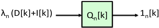
For each constraint , define a virtual queue that is updated on frames by:
| (18) |
The initial condition can be any non-negative value. For simplicity, it is assumed throughout that for all . The update (18) can be viewed as a discrete time queueing equation, where is the backlog on frame , is an effective amount of “new arrivals,” and is the amount of “offered service” (see Fig. 2). The intuition is that if all virtual queues are stable, then the average “arrival rate” must be less than or equal to the average “service rate” , which ensures the desired constraint (17). This is made precise in the following lemma.
Lemma 2
(Virtual Queues) Suppose has update equation given by (18), with any non-negative initial condition.
a) For all we have:
| (19) |
b) If with probability 1, then:
| (20) |
c) If , then:
| (21) |
where , , are defined:
Proof:
Inequality (19) shows that the value bounds the amount by which the desired constraint for class is violated by the time averages achieved over the first frames. Suppose that , , and have frame averages that converge to constants , , with probability 1. Part (c) of Lemma 2 indicates that if for all , then for all .
II-G The Drift-Plus-Penalty Ratio
To stabilize the queues while minimizing time average power, we use Lyapunov optimization theory, which gives rise to the drift-plus-penalty ratio algorithm [1]. First define as the sum of the squares of all queues on frame (divided by for convenience later):
is often called a Lyapunov function, and acts as a scalar measure of the size of the queues. Intuitively, keeping small leads to stable queues, and we should take actions that tend to shrink from one frame to the next. Define as the Lyapunov drift, being the difference in the Lyapunov function from one frame to the next:
Taking actions to minimize every frame can be shown to ensure the desired constraints are satisfied whenever it is possible to satisfy them, but does not incorporate power minimization. To incorporate this, every frame we observe the current queue vector and choose control actions to minimize a bound on the following drift-plus-penalty ratio:
where is a non-negative parameter that weights the extent to which power minimization is emphasized. The intuition is that the numerator incorporates both drift and energy. The denominator “normalizes” this by the expected frame size, with the understanding that average power must include both energy and frame size. We soon show that this intuition is correct, in that all desired time average constraints are satisfied, and the time average power is within of the optimal value . Hence, average power can be pushed arbitrarily close to optimal by using a sufficiently large value of . The tradeoff is that average queue sizes grow with , which impacts the convergence time required to satisfy the desired constraints.
The drift-plus-penalty ratio method was first developed for the context of restless bandit systems in [8][9]. The method was used for optimization of renewal systems in [1][2], which treat problems similar to those considered in this paper. In the special case when all frame sizes are fixed and equal to one unit of time (a time slot), and when , the method reduces to observing queues every slot and taking actions to minimize a bound on . This is the rule that generates the classic max-weight scheduling algorithms for queue stability (without performance optimization), developed by Tassiulas and Ephremides in [10][11]. For systems with unit time slots but with , the drift-plus-penalty ratio technique reduces to the drift-plus-penalty technique of [12][13][14], which treats joint queue stability and penalty minimization in systems with unit size slots.
II-G1 Bounding the Drift-Plus-Penalty Ratio
To construct an explicit algorithm, we first bound the drift-plus-penalty ratio.
Lemma 3
For all frames , all possible , and under any decisions for , we have:
| (22) | |||||
where is a constant that satisfies the following for all possible and all policies:
Such a constant exists by the second moment boundedness assumptions (1).
Proof:
Note by iterated expectations that (similar to (7)):222In more detail, by iterated expectations we have , and because is conditionally independent of the past given the current used.
Thus, the denominator is common for all terms of inequality (22), and it suffices to prove:
| (23) |
To this end, by squaring (18) and noting that , we have for each :
Summing the above over and using the definition of gives:
Taking conditional expectations given and using the bound proves (23). ∎
II-G2 The Task Scheduling Algorithm
Our algorithm takes actions every frame to minimize the last two terms on the right-hand-side of the drift-plus-penalty ratio bound (22). The only part of these terms that we have control over on frame (given the observed ) is given below:
Recall from Lemma 1 that minimizing the above ratio of expectations is accomplished over a deterministic choice of . Thus, every frame we perform the following:
II-G3 Steps to minimize (24)
Here we elaborate on how to perform the minimization in (24) for each frame . For each and , define as the value of that minimizes (24), given that we have . It is easy to see that:
Now define by:
Then we choose as the minimizer of over and , breaking ties arbitrarily, and choose . Note that this algorithm chooses or on every frame . Nevertheless, it results in a frame average that approaches optimality for large .
II-H Performance of the Task Scheduling Algorithm
For simplicity, the performance theorem is presented in terms of zero initial conditions. It is assumed throughout that the problem (3)-(6) is feasible, so that it is possible to satisfy the constraints.
Theorem 1
Suppose for all , and that the problem (3)-(6) is feasible. Then under the above task scheduling algorithm:
a) For all frames we have:333The right-hand-side in (25) can be simplified to , since all frames are at least in size.
| (25) |
where is defined in Lemma 3, is the minimum power solution for the problem (3)-(6), and , , are defined by:
b) The desired constraints (20) and (21) are satisfied for all . Further, we have for each frame :
| (26) |
where is the norm of the queue vector (being at least as large as each component ), and is a constant that satisfies the following for all frames :
Such a constant exists because the second moments (and hence first moments) are bounded.
In the special case of a deterministic system, all expectations of the above theorem can be removed, and the results hold deterministically for all frames . Theorem 1 indicates that average power can be pushed arbitrarily close to , using the parameter that affects an performance gap given in (25). The tradeoff is that increases the expected size of as shown in (26), which bounds the expected deviation from the th constraint during the first frames (recall (19) from Lemma 2). Under a mild additional “Slater-type” assumption that ensures all constraints can be satisfied with “-slackness,” a stronger result on the virtual queues can be shown, namely, that the same algorithm yields queues with average size [1]. This typically ensures a tighter constraint tradeoff than that given in (26). A related improved tradeoff is explored in more detail in Section III-C.
Proof:
(Theorem 1 part (a)) Given for frame , our control decisions minimize the last two terms in the right-hand-side of the drift-plus-penalty ratio bound (22), and hence:
| (27) | |||||
where , , , are from any alternative (possibly randomized) decisions that can be made on frame . Now recall the existence of stationary and randomized decisions that yield (15)-(16). In particular, these decisions are independent of queue backlog and thus yield (from (15)):
and for all we have (from (16)):
Plugging the above into the right-hand-side of (27) yields:
Rearranging terms gives:
Taking expectations of the above (with respect to the random ) and using the law of iterated expectations gives:
| (28) |
The above holds for all . Fixing a positive integer and summing (28) over yields, by the definition :
Noting that and and using the definitions of , , yields:
Rearranging terms yields the result of part (a). ∎
Proof:
(Theorem 1 part (b)) To prove part (b), note from (28) we have:
Summing the above over gives:
Using the definition of and noting that gives:
Thus, we have . Jensen’s inequality for ensures , and so for all positive integers :
| (29) |
Taking a square root of both sides of (29) and dividing by proves (26). From (26) we have for each :
and hence by Lemma 2 we know constraint (21) holds. Further, in [15] it is shown that (29) together with the fact that second moments of queue changes are bounded implies with probability 1. Thus, (20) holds. ∎
II-I Simulation
We first simulate the task scheduling algorithm for the simple deterministic system with one class and one constraint, as described in Section II-D. The and functions are defined in (8)-(9), and the goal is to minimize average power subject to a processing rate constraint . We already know the optimal power is . We expect the algorithm to approach this optimal power as is increased, and to approach the desired behavior of using for all , meeting the constraint with equality, and using for of the frames. This is indeed what happens, although in this simple case the algorithm seems insensitive to the parameter and locks into a desirable periodic schedule even for very low (but positive) values. Using and one million frames, the algorithm gets average power , uses a fraction of time , has average idle time , and yields a processing rate (almost exactly equal to the desired constraint of ). Increasing yields similar performance. The constraint is still satisfied when we decrease the value of , but average power degrades (being for ).
We next consider a system with 10 classes of tasks and two processing modes. The energy and delay characteristics for each class and mode are:
| Mode 1: | (30) | ||||
| Mode 2: | (31) |
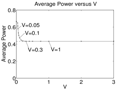
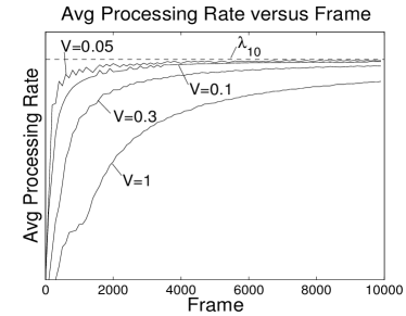
so that mode 1 uses less energy but takes longer than mode 2, and the computational requirements for each class increase with . We assume desired rates are given by for , for some positive value . The problem is feasible whenever . We use and run the simulation for 10 million frames. Fig. 4 shows the resulting average power as is varied between and , which converges to near optimal after . All 10 processing rate constraints are met within 5 decimal points of accuracy after the 10 million frames. An illustration of how convergence time is affected by the parameter is shown in Fig. 4, which illustrates the average processing rate for class 10, as compared to the desired constraint . It is seen, for example, that convergence is faster for than for . Convergence times can be improved using non-zero initial queue backlog and the theory of place holder backlog in [1], although we omit this topic for brevity.
III Optimization with General Attributes
This section generalizes the problem to allow time average optimization for abstract attributes. Consider again a frame-based system with frame index . Every frame , the controller makes a control action , chosen within an abstract set of allowable actions. The action affects the frame size and an attribute vector . Specifically, assume these are random functions that are conditionally independent of the past given the current decision, with mean values given by functions and for all :
Similar to the previous section, it is assumed there is a minimum frame size such that for all , and that second moments are bounded by a constant , regardless of the policy . The joint distribution of is otherwise arbitrary.
Define frame averages and by:
As discussed in Section II-B, the value represents the time average associated with attribute . The general problem is then:
| Minimize: | (32) | ||||
| Subject to: | (34) | ||||
where are given constants that specify the desired time average constraints.
III-A Mapping to the Task Scheduling Problem
To illustrate the generality of this framework, this subsection uses the new notation to exactly represent the task scheduling problem from Section II. For that problem, one can define the control action to have the form , and the action space is then the set of all such that , , and .
The frame size is , and is given by:
We then define as the energy expended in frame , so that and . There are constraints, so define . To express the desired constraints in the form , one can define and for each , and . Alternatively, one could define and enforce the constraint for all .
This general setup provides more flexibility. For example, suppose the idle state does not use 0 energy, but operates at a low power and expends total energy on frame . Then total energy for frame can be defined as , where is the energy spent in the busy period. The setup can also handle systems with multiple idle mode options, each providing a different energy savings but incurring a different wakeup time.
III-B The General Algorithm
The algorithm for solving the general problem (32)-(34) is described below. Each constraint in (34) is treated using a virtual queue with update:
| (35) |
Defining and as before (in Section II-G) leads to the following bound on the drift-plus-penalty ratio, which can be proven in a manner similar to Lemma 3:
| (36) |
where is a constant that satisfies the following for all and all possible actions :
Every frame, the controller observes queues and takes an action that minimizes the second term on the right-hand-side of (36). We know from Lemma 1 that minimizing the ratio of expectations is accomplished by a deterministic selection of . The resulting algorithm is:
-
•
Observe and choose to minimize (breaking ties arbitrarily):
(37) -
•
Update virtual queues for each via (35).
One subtlety is that the expression (37) may not have an achievable minimum over the general (possibly infinite) set (for example, the infimum of the function over the open interval is not achievable over that interval). This is no problem: Our algorithm in fact works for any approximate minimum that is an additive constant away from the exact infimum every frame (for any arbitrarily large constant ). This effectively changes the “” constant in our performance bounds to a new constant “” [1]. Let represent the optimal ratio of for the problem (32)-(34). As before, it can be shown that if the problem is feasible (so that there exists an algorithm that can achieve the constraints (34)-(34)), then any -additive approximation of the above algorithm satisfies all desired constraints and yields , which can be pushed arbitrarily close to as is increased, with the same tradeoff in the queue sizes (and hence convergence times) with . The proof of this is similar to that of Theorem 1, and is omitted for brevity (see [1][2] for the full proof).
III-C Random Task Arrivals and Flow Control
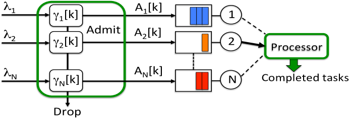
Again consider a system with classes of tasks, as in Section II. Each frame again has a busy period of duration and an idle period of duration as in Fig. 1. However, rather than always having tasks available for processing, this subsection assumes tasks arrive randomly with rates , where is the rate of task arrivals per unit time (see Fig. 5). At the beginning of each busy period, the controller chooses a variable that specifies which type of task is performed. However, can now take values in the set , where is a null choice that selects no task on frame . If , the busy period has some positive size and may spend a small amount of energy to power the electronics, but does not process any task. The mode selection variable takes values in the same set as before. The idle time variable is again chosen in the interval .
Further, for each we introduce flow control variables , chosen in the interval . The variable represents the probability of admitting each new randomly arriving task of class on frame (see Fig. 5). This enables the system to drop tasks if the raw arrival rates cannot be supported. Let be the vector of these variables.
We thus have , with action space being the set of all such that , , , and for . Define and as the energy and busy period duration for frame . Assume depends only on , and depends only on , with averages given by functions and :
Finally, for each , define as the random number of new arrivals admitted on frame , which depends on the total frame size and the admission probability . Formally, assume the arrival vector is conditionally independent of the past given the current used, with expectations:
| (38) |
The assumption on independence of the past holds whenever arrivals are independent and Poisson, or when all frame sizes are an integer number of fixed size slots, and arrivals are independent and identically distributed (i.i.d.) over slots with some general distribution.
We seek to maximize a weighted sum of admission rates subject to supporting all of the admitted tasks, and to maintaining average power to within a given positive constant :
| Maximize: | (39) | ||||
| Subject to: | (42) | ||||
where are a collection of positive weights that prioritize the different classes in the optimization objective.
We thus have constraints. To treat this problem, define , so that . Further define , for , and as:
Then:
Note that the above problem does not specify any explicit queueing for the randomly arriving tasks. The algorithm will in fact construct explicit queues (so that the virtual queues can be viewed as actual queues). Note also that the constraint does not allow restrictions on actions based on the queue state, such as when the queue is empty or not. Thus, in principle, we allow the possibility of “processing” a task of class even when there is no such task available. In this case, we assume this processing is still costly, in that it incurs time equal to and energy equal to . Our algorithm will naturally learn to avoid the inefficiencies associated with such actions.
III-C1 The Dynamic Algorithm for Random Task Arrivals
To enforce the constraints for each , define queue with update:
| (43) |
To enforce , define a virtual queue with update:
| (44) |
It can be seen that the queue update (43) is the same as that of an actual queue for class tasks, with random task arrivals and task service . The minimization of (37) then becomes the following: Every frame , observe queues and . Then choose , , , and for all to minimize:
| (45) |
After a simplifying cancellation of terms, it is easy to see that the decisions can be separated from all other decisions (see Exercise 2). The resulting algorithm then observes queues and every frame and performs the following:
-
•
(Flow Control) For each , choose as:
(46) -
•
(Task Scheduling) Choose , , to minimize:
(47) - •
The minimization problem (47) is similar to (24), and can be carried out in the same manner as discussed in Section II-G. A key observation about the above algorithm is that it does not require knowledge of the arrival rates . Indeed, the terms cancel out of the minimization, so that the flow control variables in (46) make “bang-bang” decisions that admit all newly arriving tasks of class on frame if , and admit none otherwise. This property makes the algorithm naturally adaptive to situations when the arrival rates change, as shown in the simulations of Section III-D.
Note that if for all , , , so that the energy associated with processing no task is less than the energy of processing any class , then the minimization in (47) will never select a class such that . That is, the algorithm naturally will never select a class for which no task is available.
III-C2 Deterministic Queue Bounds and Constraint Violation Bounds
In addition to satisfying the desired constraints and achieving a weighted sum of admitted rates that is within of optimality, the flow control structure of the task scheduling algorithm admits deterministic queue bounds. Specifically, assume all frame sizes are bounded by a constant , and that the raw number of class arrivals per frame (before admission control) is at most . By the flow control policy (46), new arrivals of class are only admitted if . Thus, assuming that , we must have for all frames . This specifies a worst-case queue backlog that is , which establishes an explicit performance-backlog tradeoff that is superior to that given in (26).
III-D Simulations and Adaptiveness of Random Task Scheduling
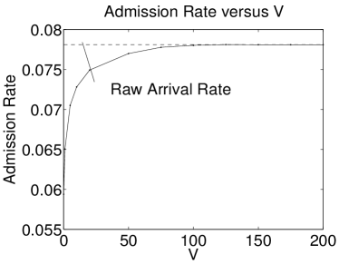
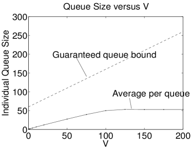
Here we simulate the dynamic task scheduling and flow control algorithm (46)-(47), using the 10-class system model defined in Section II-I with functions given in (30)-(31). For consistency with that model, we remove the option, so that the decision (31) chooses , incurring one unit of energy, in case no tasks are available. Arrivals are from independent Bernoulli processes with rates for each class , with . We use weights for all , so that the objective is to maximize total throughput, and , which we know is feasible from results in Fig. 4 of Section II-I. Thus, we expect the algorithm to learn to admit everything, so that the admission rate approaches the total arrival rate as is increased. We simulate for 10 million frames, using in the interval from to . Results are shown in Figs. 7 and 7. Fig 7 shows the algorithm learns to admit everything for large (100 or above), and Fig. 7 plots the resulting average queue size (in number of tasks) per queue, together with the deterministic bound (where in this case because there is at most one arrival per slot, and the largest possible frame is ). The average power constraint was satisfied (with slackness) for all cases. The average queue size in Fig. 7 grows linearly with until , when it saturates by admitting everything. The saturation value is the average queue size associated with admitting the raw arrival rates directly.
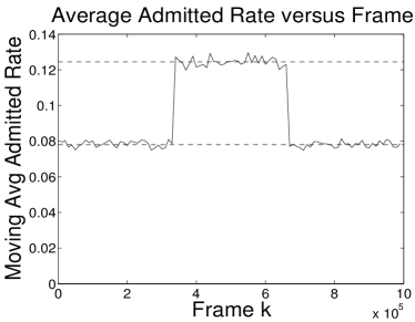
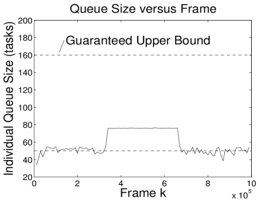
We now illustrate that the algorithm is robust to abrupt rate changes. We consider the same system as before, run over 10 million frames with . However, we break the simulation timeline into three equal size phases. During the first and third phase, we use arrival rates for , where as in the previous experiment. Then, during the second (middle) phase, we double the rates to , where . Because , these rates are infeasible and the algorithm must learn to optimally drop tasks so as to maximize the admission rate subject to the power constraint. Recall that the algorithm is unaware of the arrival rates and must adapt to the existing system conditions. The results are shown in Figs. 9 and 9. Fig. 9 shows a moving average admission rate versus time. During the first and third phases of the simulation, we have and the admitted rates are close to the raw arrival rate (shown as the lower dashed horizontal line). During the middle interval (with ), the algorithm quickly adapts to the increased arrivals and yields admitted rates that are close to those that should be used in a system with loading always (shown as the higher dashed horizontal line). Fig. 9 plots the corresponding moving average queue backlog per queue. The lower dashed horizontal line indicates the value of average backlog that would be achieved in a system with loading always. Also shown is the deterministic queue bound , which holds for all frames, regardless of the raw arrival rates.
III-E Task Scheduling: Extensions and Further Reading
This section considered minimizing time averages subject to time average constraints. Extended techniques for minimizing convex functions of time average vectors (or maximizing concave functions) subject to similar constraints are treated in the renewal optimization theory of [1][2]. This is useful for extending the flow control problem (39)-(42) to optimize a sum of concave utility functions of the time average admission rates for each class:
Using logarithmic functions leads to proportional fairness [16], while other fairness properties are achieved with other concave functions [17][18][19]. Related utility optimization for particular classes of wireless systems with fixed size frames of slots, and with probabilistic reception every slot, is treated using a different technique in [20][21]. Related work on utility optimal scheduling for single-slot data networks is treated using convex optimization in [22][23][24][25], stochastic “primal-dual” algorithms in [26][27][28][29][30], and stochastic “dual” algorithms in [12][31][32][13][33].
For the problem with random arrivals, queueing delay can often be improved by changing the constraint of (42) to , for some . This specifies that the output processing rate should be larger than the arrival rate. However, unlike the case , such a constraint yields a queue that contains some “fake” tasks, and can lead to decisions that serve the queue when no actual tasks are available. This can be overcome using the theory of -persistent service queues in [34][35].
Note that our flow control algorithm rewards admission of new data on each frame. This fits the general framework of this section, where attributes are (possibly random) functions of the control action . One might attempt to solve the problem by defining a reward upon completion of service. This does not fit our framework: That is because the algorithm might “complete” a service in a queue that is empty, simply to accumulate the “fake” reward. One could eliminate fake rewards by an augmented model that allows rewards and/or action spaces that depend on the current backlog, although this creates a much more complex Markov decision model that is easily avoided by defining rewards at admission. However, there are some problems that require such a reward structure, such as problems of stock market trading where prior ownership of a particular stock is required to reap the benefits of selling at an observed desirable price. These problems can be treated with a modified Lyapunov function of the form , which pushes backlog towards a non-empty state . This approach is used for stock trading [36], inventory control [37], energy harvesting [38], and smart-grid energy management [39]. The first algorithms for optimal energy harvesting used a related technique [40], and related problems in processing networks that assemble components by combining different sub-components are treated in [41][42].
III-F Exercises for Section III
Exercise 1
Consider a system with classes, each of which always has new tasks available. Every frame we choose a class , and select a single task of that class for processing. We can process using mode . The result yields frame size , energy , and processing quality . Design an algorithm that selects and every frame to maximize subject to an average power constraint and to a processing rate constraint of at least for each class .
Exercise 2
Exercise 3
Consider the flow control and task scheduling algorithm (46)-(47), and recall that for all and all frames , where . Suppose there is a constant such that for all , and that for all , .
a) Show that the minimization of (47) chooses whenever .
b) Suppose there is a constant such that for all . Conclude that for all frames .
Exercise 4
Consider the same general attributes of Section III, with for . State the algorithm for solving the problem of minimizing subject to . Hint: Define appropriate attributes on a system with an “effective” frame size of 1 every frame, and minimize subject to for .
Exercise 5
Modify the task scheduling algorithm of Section II-G to allow the controller to serve more than one task per frame. Specifically, every frame the controller chooses a service action from a set of possible actions. Each service action determines a clearance vector , where is the number of tasks of type served if action is used on a given frame. It also incurs a delay and energy .
Exercise 6
Consider the linear fractional problem of finding a vector to solve:
| Minimize: | ||||
| Subject to: | ||||
Assume constants , , , are given, that , and that for all . Treat this as a time average problem with action , action space , frame size , and where we seek to minimize subject to for all .
a) State the drift-plus-penalty ratio algorithm (37) for this, and conclude that:
for some finite constant , where is the optimal value of the objective function, and . Thus, the limiting time average satisfies the constraints and is within from optimality. Your answer should solve for values such that on frame we choose over to minimize . Note: In Appendix B it is shown that this minimization is performed as follows: Define and . For all , choose if , and if . Next, temporarily select for all . Then rank order the indices from smallest to largest value of , and, using this order, greedily change from to if it improves the solution. We stop when we reach the first index in the rank ordering that does not improve the solution.
b) Note that the case and for is a linear program. Give an explicit decision rule for each in this case (the solution should be separable for each ).
IV Reacting to Randomly Observed Events
Consider a problem with general attributes and frame size for each frame , as in Section III. However, now assume the controller observes a random event at the beginning of each frame , and this can influence attributes and frame sizes. The value of can represent a vector of channel states and/or prices observed for frame . Assume is independent and identically distributed (i.i.d.) over frames. The controller chooses an action , where the action space possibly depends on the observed . Values of are conditionally independent of the past given the current and , with mean values:
The goal is to solve the following optimization problem:
| Minimize: | (48) | ||||
| Subject to: | (50) | ||||
As before, the constraints are satisfied via virtual queues for :
| (51) |
The random observations make this problem more complex that those considered in previous sections of this paper. We present two different algorithms from [1][2].
Algorithm 1: Every frame , observe and and choose to minimize the following ratio of expectations:
| (52) |
Then update the virtual queues via (51).
Algorithm 2: Define , and define for as a running ratio of averages over past frames:
| (53) |
Then every frame , observe , , and , and choose to minimize the following function:
| (54) |
Then update the virtual queues via (51).
IV-A Comparison of Algorithms 1 and 2
Both algorithms are introduced and analyzed in [1][2], where they are shown to satisfy the desired constraints and yield an optimality gap of . Algorithm 1 can be analyzed in a manner similar to the proof of Theorem 1, and has the same tradeoff with as given in that theorem. However, the ratio of expectations (52) is not necessarily minimized by observing and choosing to minimize the deterministic ratio given . In fact, the minimizing policy depends on the (typically unknown) probability distribution for . A more complex bisection algorithm is needed for implementation, as specified in [1][2].
Algorithm 2 is much simpler and involves a greedy selection of based only on observation of , without requiring knowledge of the probability distribution for . However, its mathematical analysis does not yield as explicit information regarding convergence time as does Algorithm 1. Further, it requires a running average to be kept starting at frame , and hence may not be as adaptive when system statistics change. A more adaptive approximation of Algorithm 2 would define the average over a moving window of some fixed number of frames, or would use an exponentially decaying average.
Both algorithms reduce to the following simplified drift-plus-penalty rule in the special case when the frame size is a fixed constant for all : Every frame , observe and and choose to minimize:
| (55) |
Then update the virtual queues via (51). This special case algorithm was developed in [14] to treat systems with fixed size time slots.
A simulation comparison of the algorithms is given in [2]. The next subsection describes an application to energy-aware computation and transmission in a wireless smart phone. Exercise 7 considers opportunistic scheduling where wireless transmissions can be deferred by waiting for more desirable channels. Exercise 8 considers an example of price-aware energy consumption for a network server that can process computational tasks or outsource them to another server.
IV-B Efficient Computation and Transmission for a Wireless Smart Device
Consider a wireless smart device (such as a smart phone or sensor) that always has tasks to process. Each task involves a computation operation, followed by a transmission operation over a wireless channel. On each frame , the device takes a new task and looks at its meta-data , being information that characterizes the task in terms of its computational and transmission requirements. Let represent the time required to observe this meta-data. The device then chooses a computational processing mode , where is the set of all mode options under . The mode and meta-data affect a computation time , computation energy , computation quality , and generate bits for transmission over the channel. The expectations of , , are:
For example, in a wireless sensor, the mode may represent a particular sensing task, where different tasks can have different qualities and thus incur different energies, times, and bits for transmission. The full conditional distribution of , given , , will play a role in the transmission stage (rather than just its conditional expectation).
The units of data must be transmitted over a wireless channel. Let be the state of the channel on frame , and assume is constant for the duration of the frame. We choose a transmission mode , yielding a transmission time and transmission energy with expectations that depend on , , and . Define random event and action . We can then define expectation functions and by:
where the above expectations are defined via the conditional distribution associated with the number of bits at the computation output, given the meta-data and computation mode selected in the computation phase (where and are included in the , information). The total frame size is thus .
The goal is to maximize frame processing quality per unit time subject to a processing rate constraint of , and subject to an average power constraint (where and are given constants). This fits the general framework with observed random events , control actions , and action space . We can define , , and , and solve the problem of minimizing subject to and . To do so, let and be virtual queues for the two constraints:
| (56) | |||||
| (57) |
Using Algorithm 2, we define and for by (53). The Algorithm 2 minimization (54) amounts to observing , , , and on each frame and choosing and to minimize:
The computation and transmission operations are coupled and cannot be separated. This yields the following algorithm: Every frame :
-
•
Observe and values , , . Then jointly choose action and , for a combined action , to minimize:
- •
Exercise 9 shows the algorithm can be implemented without if the goal is changed to maximize , rather than . Further, the computation and transmission decisions can be separated if the system is modified so that the bits generated from computation are handed to a separate transmission layer for eventual transmission over the channel, rather than requiring transmission on the same frame, similar to the structure used in Exercise 8.
IV-C Exercises for Section IV
Exercise 7
(Energy-Efficient Opportunistic Scheduling [14]) Consider a wireless device that operates over fixed size time slots . Every slot , new data of size bits arrives and is added to a queue. The data must eventually be transmitted over a time-varying channel. At the beginning of every slot , a controller observes the channel state and allocates power for transmission, enabling transmission of bits, where for some given function . Assume is chosen so that for some constant . We want to minimize average power subject to supporting all data, so that . Treat this as a problem with all frames equal to 1 slot, observed random events , and actions . Design an appropriate queue update and power allocation algorithm, using the policy structure (55).
Exercise 8
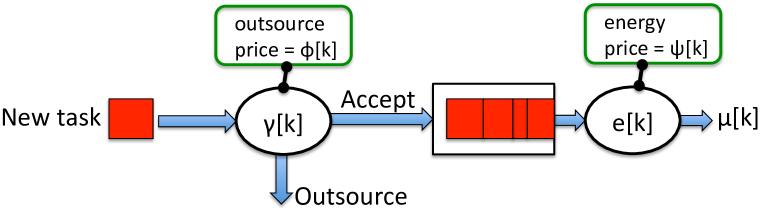
(Energy Prices and Network Outsourcing) Consider a computer server that operates over fixed length time slots . Every slot , a new task arrives and has size (if no task arrives then ). The server decides to either accept the task, or outsource it to another server (see Fig. 10). Let be a binary decision variable that is 1 if the server accepts the task on slot , and zero else. Define as the total workload admitted on slot , which is added to the queue of work to be done. Let be the (possibly time-varying) cost per unit size for outsourcing, so the outsourcing cost is . Every slot , the server additionally decides to process some of its backlog by purchasing an amount of energy at a per-unit energy price , serving units of backlog with cost , where is some given function. Assume is chosen in some interval . The goal is to minimize time average cost subject to supporting all tasks, so that . Treat this as a problem with all frames equal to 1 slot, observed random events , actions , and action space being the set of all such that and . Design an appropriate queue and state the dynamic algorithm (55) for this problem. Show that it can be implemented without knowledge of the probability distribution for , and that the and decisions are separable.
V Conclusions
This paper presents a methodology for optimizing time averages in systems with variable length frames. Applications include energy and quality aware task scheduling in smart phones, cost effective energy management at computer servers, and more. The resulting algorithms are dynamic and often do not require knowledge of the probabilities that affect system events. While the performance theorem of this paper was stated under simple i.i.d. assumptions, the same algorithms are often provably robust to non-i.i.d. situations, including situations where the events are non-ergodic [1]. Simulations in Section III-D show examples of how such algorithms adapt to changes in the event probabilities. Exercises in this paper were included to help readers learn to design dynamic algorithms for their own optimization problems.
The solution technique of this paper uses the theory of optimization for renewal systems from [1][2], which applies to general problems. Performance for individual problems can often be improved using enhanced techniques, such as using place-holder backlog, exponential Lyapunov functions, LIFO scheduling, and -persistent service queues, as discussed in [1] and references therein. However, the drift-plus-penalty methodology described in this paper provides much of the insight needed for these more advanced techniques. It is also simple to work with and typically yields desirable solution quality and convergence time.
Appendix A — Bounded Moment Convergence Theorem
This appendix provides a bounded moment convergence theorem that is often more convenient than the standard Lebesgue dominated convergence theorem (see, for example, [43] for the standard Lebesgue dominated convergence theorem). We are unaware of a statement and proof in the literature, so we give one here for completeness. Let be a random process defined either over non-negative real numbers , or discrete time . Recall that converges in probability to a constant if for all we have:
Theorem 2
Suppose there is a real number such that converges to in probability. Further suppose there are finite constants , such that for all we have . Then .
Proof:
Without loss of generality, assume (else, we can define ). Fix . By definition of converging to in probability, we have:
| (58) |
Further, for all we have , and so:
| (59) |
We want to show the final term in the right-hand-side above converges to when . To this end, note that for all we have:
| (60) | |||||
where (60) follows by Jensen’s inequality applied to the conditional expectation of the function , where is convex over . Multiplying inequality (60) by yields:
Taking a limit of the above as and using (58) yields:
It follows that:
Using this equality and taking a of (59) yields . This holds for all , and so . Similarly, it can be shown that . Thus, . ∎
Recall that convergence with probability 1 is stronger than convergence in probability, and so the above result also holds if with probability 1. Theorem 2 can be applied to the case when with probability 1, for some finite constant , and when there is a constant such that for all . Indeed, one can define for and use the Cauchy-Schwartz inequality to show for all , and so .
Appendix B — The Decision Rule for Linear Fractional Programming
This appendix proves optimality of the decision rule for online linear fractional programming given in Exercise 6. Specifically, suppose we have real numbers , a positive real number , and non-negative real numbers . The goal is to solve the following problem:
| Minimize: | ||||
| Subject to: |
To this end, define disjoint sets and that partition the indices as follows:
Then the objective function can be written:
The denominator is always positive, and so regardless of the values for , the first term on the right-hand-side above is minimized by choosing for all such that if , and if . Let for denote these decisions. It remains only to choose optimal values for . Define . We want to solve the following:
| Minimize: | (61) | ||||
| Subject to: | (62) |
Define as the minimum value for the objective function in the problem (61)-(62).
Proof:
Let be an optimal solution to (61)-(62), so that for all and:
Define and by:
so that . Now take any . It suffices so show we can change to , as defined in (63), without changing the ratio from its value . Indeed, if this is true, then we can sequentially change each component to without changing the ratio, and so is also an optimal solution.
To this end, define as the corresponding ratio with replaced with . We show that . Clearly by definition of as the minimum ratio. To show the opposite inequality, define , and note that:
| (64) | |||||
Note that , and hence the second term on the right-hand-side of (64) is non-positive if . In the case , then by (63) we have . Thus, and . Thus, the second term in the right-hand-side of (64) is non-positive and so . In the opposite case , then and so , . Thus, the second term on the right-hand-side of (64) is again non-positive, so that . ∎
Now rank order the indices from smallest to largest value of , breaking ties arbitrarily. The solution of Lemma 4 has the form where for the first indices in this rank order, and for the remaining indices, for some value (where is the size of set ). Define as the value of the ratio when for the first indices in the rank order, and for the remaining indices in . Start with . According to the rank ordering of , successively change from to if it strictly decreases the ratio, computing , , and so on, until we reach the first index that does not improve the ratio. By an argument similar to (64), it is easy to see that this can only occur at an index such that is greater than or equal to the current ratio, which means it is also greater than or equal to (since by definition, is less than or equal to any achievable ratio). Thus, all indices that come after in the rank ordering also have , and this greedy approach has thus arrived at the solution (63).
References
- [1] M. J. Neely. Stochastic Network Optimization with Application to Communication and Queueing Systems. Morgan & Claypool, 2010.
- [2] M. J. Neely. Dynamic optimization and learning for renewal systems. Proc. Asilomar Conf. on Signals, Systems, and Computers, Nov. 2010.
- [3] E. Grochowski, R. Ronen, J. Shen, and H. Wang. Best of both latency and throughput. Proc. IEEE Conf. on Computer Design (ICCD), pp. 236-243, October 2004.
- [4] M. Annavaram, E. Grochowski, and J. Shen. Mitigating amdahl’s law through epi throttling. Proc. 32nd International Symposium on Computer Architecture (ISCA), pp. 298-309, June 2005.
- [5] R. Gallager. Discrete Stochastic Processes. Kluwer Academic Publishers, Boston, 1996.
- [6] S. Ross. Introduction to Probability Models. Academic Press, 8th edition, Dec. 2002.
- [7] S. Boyd and L. Vandenberghe. Convex Optimization. Cambridge University Press, 2004.
- [8] C. Li and M. J. Neely. Network utility maximization over partially observable markovian channels. Arxiv Technical Report: arXiv:1008.3421v1, Aug. 2010.
- [9] C. Li and M. J. Neely. Network utility maximization over partially observable markovian channels. Proc. Intl. Symposium on Modeling and Optimization in Mobile, Ad Hoc, and Wireless Networks (WiOpt), May 2011.
- [10] L. Tassiulas and A. Ephremides. Stability properties of constrained queueing systems and scheduling policies for maximum throughput in multihop radio networks. IEEE Transacations on Automatic Control, vol. 37, no. 12, pp. 1936-1948, Dec. 1992.
- [11] L. Tassiulas and A. Ephremides. Dynamic server allocation to parallel queues with randomly varying connectivity. IEEE Transactions on Information Theory, vol. 39, no. 2, pp. 466-478, March 1993.
- [12] M. J. Neely. Dynamic Power Allocation and Routing for Satellite and Wireless Networks with Time Varying Channels. PhD thesis, Massachusetts Institute of Technology, LIDS, 2003.
- [13] L. Georgiadis, M. J. Neely, and L. Tassiulas. Resource allocation and cross-layer control in wireless networks. Foundations and Trends in Networking, vol. 1, no. 1, pp. 1-149, 2006.
- [14] M. J. Neely. Energy optimal control for time varying wireless networks. IEEE Transactions on Information Theory, vol. 52, no. 7, pp. 2915-2934, July 2006.
- [15] M. J. Neely. Queue stability and probability 1 convergence via lyapunov optimization. Arxiv Technical Report, arXiv:1008.3519v2, Oct. 2010.
- [16] F. Kelly. Charging and rate control for elastic traffic. European Transactions on Telecommunications, vol. 8, no. 1 pp. 33-37, Jan.-Feb. 1997.
- [17] J. Mo and J. Walrand. Fair end-to-end window-based congestion control. IEEE/ACM Transactions on Networking, vol. 8, no. 5, Oct. 2000.
- [18] A. Tang, J. Wang, and S. Low. Is fair allocation always inefficient. Proc. IEEE INFOCOM, March 2004.
- [19] W.-H. Wang, M. Palaniswami, and S. H. Low. Application-oriented flow control: Fundamentals, algorithms, and fairness. IEEE/ACM Transactions on Networking, vol. 14, no. 6, Dec. 2006.
- [20] I. Hou and P. R. Kumar. Utility maximization for delay constrained qos in wireless. Proc. IEEE INFOCOM, March 2010.
- [21] I. Hou, V. Borkar, and P. R. Kumar. A theory of qos for wireless. Proc. IEEE INFOCOM, April 2009.
- [22] F.P. Kelly, A.Maulloo, and D. Tan. Rate control for communication networks: Shadow prices, proportional fairness, and stability. Journ. of the Operational Res. Society, vol. 49, no. 3, pp. 237-252, March 1998.
- [23] S. H. Low. A duality model of TCP and queue management algorithms. IEEE Trans. on Networking, vol. 11, no. 4, pp. 525-536, August 2003.
- [24] L. Xiao, M. Johansson, and S. P. Boyd. Simultaneous routing and resource allocation via dual decomposition. IEEE Transactions on Communications, vol. 52, no. 7, pp. 1136-1144, July 2004.
- [25] X. Lin and N. B. Shroff. Joint rate control and scheduling in multihop wireless networks. Proc. of 43rd IEEE Conf. on Decision and Control, Paradise Island, Bahamas, Dec. 2004.
- [26] H. Kushner and P. Whiting. Asymptotic properties of proportional-fair sharing algorithms. Proc. of 40th Annual Allerton Conf. on Communication, Control, and Computing, 2002.
- [27] R. Agrawal and V. Subramanian. Optimality of certain channel aware scheduling policies. Proc. 40th Annual Allerton Conference on Communication , Control, and Computing, Monticello, IL, Oct. 2002.
- [28] A. Stolyar. Maximizing queueing network utility subject to stability: Greedy primal-dual algorithm. Queueing Systems, vol. 50, no. 4, pp. 401-457, 2005.
- [29] A. Eryilmaz and R. Srikant. Joint congestion control, routing, and mac for stability and fairness in wireless networks. IEEE Journal on Selected Areas in Communications, Special Issue on Nonlinear Optimization of Communication Systems, vol. 14, pp. 1514-1524, Aug. 2006.
- [30] Q. Li and R. Negi. Scheduling in wireless networks under uncertainties: A greedy primal-dual approach. Arxiv Technical Report: arXiv:1001:2050v2, June 2010.
- [31] M. J. Neely, E. Modiano, and C. Li. Fairness and optimal stochastic control for heterogeneous networks. Proc. IEEE INFOCOM, March 2005.
- [32] A. Eryilmaz and R. Srikant. Fair resource allocation in wireless networks using queue-length-based scheduling and congestion control. Proc. IEEE INFOCOM, March 2005.
- [33] A. Ribeiro and G. B. Giannakis. Separation principles in wireless networking. IEEE Transactions on Information Theory, vol. 56, no. 9, pp. 4488-4505, Sept. 2010.
- [34] M. J. Neely, A. S. Tehrani, and A. G. Dimakis. Efficient algorithms for renewable energy allocation to delay tolerant consumers. 1st IEEE International Conference on Smart Grid Communications, Oct. 2010.
- [35] M. J. Neely. Opportunistic scheduling with worst case delay guarantees in single and multi-hop networks. Proc. IEEE INFOCOM, 2011.
- [36] M. J. Neely. Stock market trading via stochastic network optimization. Proc. IEEE Conference on Decision and Control (CDC), Atlanta, GA, Dec. 2010.
- [37] M. J. Neely and L. Huang. Dynamic product assembly and inventory control for maximum profit. Proc. IEEE Conf. on Decision and Control (CDC), Atlanta, GA, Dec. 2010.
- [38] L. Huang and M. J. Neely. Utility optimal scheduling in energy harvesting networks. Proc. Mobihoc, May 2011.
- [39] R. Urgaonkar, B. Urgaonkar, M. J. Neely, and A. Sivasubramaniam. Optimal power cost management using stored energy in data centers. Proc. SIGMETRICS, June 2011.
- [40] M. Gatzianas, L. Georgiadis, and L. Tassiulas. Control of wireless networks with rechargeable batteries. IEEE Transactions on Wireless Communications, vol. 9, no. 2, pp. 581-593, Feb. 2010.
- [41] L. Jiang and J. Walrand. Scheduling and Congestion Control for Wireless and Processing Networks. Morgan & Claypool, 2010.
- [42] L. Huang and M. J. Neely. Utility optimal scheduling in processing networks. Proc. IFIP, Performance, 2011.
- [43] D. Williams. Probability with Martingales. Cambridge Mathematical Textbooks, Cambridge University Press, 1991.