Secret Key Generation Via Localization and Mobility

Abstract

We consider secret key generation from relative localization information of a pair of nodes in a mobile wireless network in the presence of a mobile eavesdropper. Our problem can be categorized under the source models of information theoretic secrecy, where the distance between the legitimate nodes acts as the observed common randomness. We characterize the theoretical limits on the achievable secret key bit rate, in terms of the observation noise variance at the legitimate nodes and the eavesdropper. This work provides a framework that combines information theoretic secrecy and wireless localization, and proves that the localization information provides a significant additional resource for secret key generation in mobile wireless networks.

I Introduction

We consider the generation of a common key in a pair of nodes, which move in $\mathbb{R}^{2}$ (continuous space) according to a stochastic mobility model. We exploit the reciprocity of the distance between a given pair of locations, view the distance between the legitimate nodes as a common randomness shared by these nodes and utilize it to generate secret key bits using the ideas from source models of secrecy [1].

Unlike the recent plethora of studies (see Section I-A for a brief list of related papers) that focuses on wireless channel reciprocity, a variety of technologies can be used for localization (e.g., ultrasound, infrared, Lidar, Radar, wireless radios), which makes distance reciprocity an additional resource for generating secret key bits. Such versatility makes the key generation systems more robust, since different technologies may have different capabilities that wireless RF does not have. For instance, narrow beam width of infrared systems would make them less susceptible to eavesdropping from different angles. Distance reciprocity is highly robust, since the distance measured between any pair of points is identical, regardless of which point the measurement originates. (e.g., when there is no line-of sight, or when different frequency bands are used each way). Yet, there are various challenges in obtaining reciprocal distance measurements.

In this paper, we analyze the theoretical limits of key generation using localization in the following system. We assume that mobile nodes obtain observations regarding the sequence of distances between them over a period of time as they move in the area. The measurements can be obtained actively through exchange of wireless radio, ultrasound, infrared beacons, or passively by processing existing video images, etc. The beacon signal may contain explicit information such as a time stamp, or the receiving node can extract other means of localization information by analyzing angle of arrival, received signal strength, etc. The nodes perform localization based on the observations of distances, and the statistics of the mobility model, and obtain estimates of their relative locations with respect to each other. Then, the nodes communicate over the public channel to agree on a secret key. The generated key bits satisfy the following three quality measures: i) reliability, ii) secrecy, and iii) randomness. For reliability, we show that the probability of mismatch between the keys generated by the legitimate nodes decays to $0$ with increasing block length. In our attacker model, we consider a passive eavesdropper, that overhears the exchanged beacons in the first phase, and the public discussion in the third phase, and tries to deduce the generated key based solely on these observations. The attacker can follow various mobility strategies in order to enhance its position statistically to reduce the achievable key rate (possibly to $0$). We assume that the attacker does not actively interfere with the observation phase, e.g., by injecting jamming signals, etc., in order not to reveal its presence. For secrecy, we consider Wyner’s notion, i.e., the rate at which mutual information on the key leaks to the eavesdropper should be arbitrarily low. For randomness, the generated key bits have to be perfectly compressed, i.e., the entropy should be equal to the number of bits it contains.

We mainly focus on information theoretic limits. Using a source model of secrecy [1], we characterize the achievable secret key bit rate in terms of observation noise parameters at the legitimate nodes and the eavesdropper under two different cases of global location information (GLI): (i) No GLI, in which the nodes do not observe their global locations directly, and (ii) perfect GLI, in which nodes have perfect observation of their global locations, through a GPS device, for example. While the bounds we provide are general for a large set of observation statistics, we further investigate the scenario in which the observation noise is i.i.d. Gaussian for all nodes: We study the observation SNR asymptotics, and show a phase-transition phenomenon for the key rate. In particular, we prove that the secret key rate grows unboundedly as the observation noise variance decays, if the eavesdropper does not obtain the angle of arrival observations. Otherwise, it is not possible to increase the secret key rate beyond a certain limit. Then, we evaluate the theoretical performance numerically for a simple grid-type model, as a function of beacon power. We also evaluate the performance for the case where the eavesdropper strategically changes its location to reduce the secret key rate. Specifically, we consider the strategy where the eavesdropper moves to the middle of its location estimates of the legitimate nodes. We show that with this strategy, the eavesdropper can significantly reduce the secret key rate compared to the case where it follows a random mobility pattern.

In summary, our main contribution is to illustrate that relative localization information can be used as an additional resource for secret key generation (see Section I-A for a comparison with related work).

I-A Related Work

Generation of secret key from relative localization information can be categorized under source model of information theoretic secrecy, which studies generation of secret key bits from common randomness observed by legitimate nodes. In his seminal paper [1], Maurer showed that, if two nodes observe correlated randomness, then they can agree on a secret key through public discussion. He provided upper and lower bounds on the achievable secret key rates. Although the bounds have been improved later [2, 3], the secret key capacity of the source model in general is still an open problem. Despite this fact, the source model has been utilized in several different settings [4, 5, 6].

There is a vast amount of literature on localization (see, e.g., [8, 9] for wireless localization, [15] for infrared localization, and [16] for ultrasound localization). There has been some focus on secure localization and position-based cryptography [10, 11, 12, 13], however, these works either consider key generation in terms of other forms of secrecy (i.e., computational secrecy), or fall short of covering a complete information theoretic analysis.

A similar line of work in wireless network secrecy considers channel identification [14] for secret key generation using wireless radios. Based on the channel reciprocity assumption, nodes at both ends experience the same channel, corrupted by independent noise. Therefore, nodes can use their channel magnitude and phase response observations to generate secret key bits from public discussion. The literature on channel identification based secret key generation is vast. The works [20, 21, 22, 23, 24, 25] study key generation with on-the-shelf devices, under 802.11 development platform using a two way radio signal exchange on the same frequency. [27], on the other hand, utilizes the fact that fading is highly correlated on locations that are less than a half wavelength apart, instead of exploiting the reciprocity. Therefore, very close nodes can use public radio signals (e.g., FM, TV, WiFi) to generate secret key bits.

In most of these works, the security analysis is based on the assumption that the channel gains are modeled as random processes, that are independent of the distances between the nodes, and are independent at locations that are more than a few wavelengths apart. While being appropriate for a non line-of-sight and highly dynamic media, these models do not capture wireless propagation in environments where attenuation is a function of the propagation distance. In such environments, an attacker that has some localization capabilities will gain a statistical advantage by estimating the channel gains based on its distance observations. If the key generation process ignores this advantage, part of the key may be recovered by the attacker and thus the key cannot be perfectly secure. For instance, Jana et. al. [21] focuses on a scenario in which secret key bits based on the received signal strength (RSSI), and show that an eavesdropper that knows the location of the legitimate nodes can launch a mobility attack to force the legitimate nodes to generate deterministic key bits, by periodically blocking and un-blocking their line-of-sight. Similarly, if the eavesdropper is close (less than a wavelength) to one of the legitimate nodes, then eavesdropper will obtain correlated information [27], therefore the generated key will not be perfectly secure, and secrecy outage occurs. The practical applicability of exploiting channel reciprocity for secret key generation has also been questioned recently in [26]. It is shown that, especially when the nodes have sufficient mobility, the eavesdropper’s and the legitimate receiver’s channel can be significantly correlated depending on the locations, which breaks the secrecy of the initial generated key.

On the other hand, key generation based on locations does not make such independence assumptions. The dependencies in the locations of the legitimate nodes and the observations of the attacker with those of the legitimate nodes are taken into account to provide provably security against a mobile eavesdropper with localization capability. Thus, the insights provided in this paper can also be valuable for the class of studies on key generation based on wireless channel reciprocity, as we show how one should capture a variety of capabilities of the attackers in finding the correct rate for the key and in designing the appropriate mechanisms to generate a truly secret key.

A word about notation: We use $[x]^{+}=\max(0,x)$ and $\|.\|$ denotes the L2-norm. A brief list of variables used in the paper can be found in Table I.

II System Model

II-A Mobility Model

We consider a simple network consisting of two mobile legitimate nodes, called user $1$ and $2$, and a possibly mobile eavesdropper $e$. We divide time uniformly into $n$ discrete slots. Let $l_{j}[i]\in{\cal L}$ be the random variable that denotes the coordinates of the location of node $j\in\{1,2,e\}$ in slot $i\in\{1,\cdots,n\}$, where nodes are restricted to the field ${\cal L}\subset\mathbb{R}^{2}$. We use the boldface notation ${\bf l}_{j}=\{l_{j}[i]\}_{i=1}^{n}$, to denote the $n$-tuple location vectors for $j\in\{1,2,e\}$. The distance between nodes $1$ and $2$ in slot $i$ is ${d}_{12}[i]=\|l_{1}[i]-l_{2}[i]\|$. Similarly, ${d}_{1e}[i]$ and ${d}_{2e}[i]$ denote the sequence of distances between nodes $(1,e)$ and nodes $(2,e)$ respectively. We use the boldface notation ${\bf d}_{12}$, ${\bf d}_{1e}$, ${\bf d}_{2e}$ for the $n$-tuple distance vectors. Note that, in any slot the nodes form a triangle in $\mathbb{R}^{2}$, as depicted in Figure 1, where $\phi_{12}[i]$ , $\phi_{21}[i]$, $\phi_{1e}[i]$, $\phi_{2e}[i]$ denote the angles with respect to some coordinate axis.

Figure 1: Legitimate nodes and the eavesdropper form a triangle.

We assume that the distances $d_{12}[i],\ d_{1e}[i],\ d_{2e}[i]$ take values in the interval $[d_{\min}~{}d_{\max}]$, since the nodes cannot be closer to each other than $d_{\min}$ due to physical restrictions, and they cannot be further than $d_{\max}$ away from each other due to their limited communication range. We assume that the location vectors ${\bf l}_{1},{\bf l}_{2},{\bf l}_{e}$ are ergodic processes. We will use the notation ${\bf s}\triangleq[{\bf l}_{1},{\bf l}_{2},{\bf l}_{e}]$ to summarize the state variables related to mobility in the system. Note that $s[i]\in{\cal L}^{3}={\cal L}\times{\cal L}\times{\cal L}$ for any $i$ .

TABLE I: List of variables

var.	Description
$n$	number of slots
$T$	number of steps in public discussion
$d_{ij}$	distance between nodes $i$ and $j$
${\cal L}\in\mathbb{R}^{2}$	the field where nodes are located
$l_{j}$	2-D location of node $j$
$\phi_{ij}$	angle between nodes $i$ and $j$
$\hat{d}_{j},\hat{\phi}_{j}$	observation of nodes $j\in\{1,2\}$ of $d_{12}$ and $\phi_{j}$
$\hat{d}_{je}$	observation of node $e$ of $d_{je}$ and $\phi_{je}$
$o_{j}$	complete observations of node $j$ based on available GLI
$s$	location triple $[l_{1},l_{2},l_{e}]$
$s^{\Delta}$	quantized version of location triple, $[l_{1}^{\Delta},l_{2}^{\Delta},l_{e}^{\Delta}]$
$\Delta$	quantization resolution
$\psi$	uniform $2-D$ quantization function
$\tilde{s}_{j}^{\Delta}$	$[\tilde{l}_{1,j}^{\Delta},\tilde{l}_{2,j}^{\Delta},\tilde{l}_{e,j}^{\Delta}]$
$\tilde{l}_{k,j}^{\Delta}$	node $j$’s estimate of $l_{k}^{\Delta}$ based on all its information
$\kappa(.,m)$	$m$-bit Gray coder
$v_{j}$	obtained binary key at node $j$ before reconciliation
$u_{j}$	obtained binary key at node $j$ after reconciliation
$q_{j}$	obtained binary key at node $j$ after universal compression
$k_{j}$	final key at node $j$ after universal hashing

II-B Localization

At each time slot, there is a period in which the legitimate nodes obtain information about their relative position with respect to each other. As discussed in Section I-A, there are various methods to establish the localization information. In this paper, we will not treat these methods separately. We will simply assume that, during measurement period $i$, when node $1$ transmits a beacon, nodes $2$ and $e$ obtain a noisy observation of $d_{12}[i]$ and $d_{1e}[i]$ respectively. Let these observation be $\hat{d}_{2}[i]$ and $\hat{d}_{1e}[i]$, respectively. Similarly, when node $2$ follows up with a beacon, nodes $1$ and $e$ obtain the distance observations $\hat{d}_{1}[i]$ and $\hat{d}_{2e}[i]$, respectively. The nodes may also independently observe their global positions, e.g., through a GPS device. They may also observe the angle they make with respect to each other, if they are equipped with direction sensitive localizers (e.g., directional antennas in wireless localization). We consider two extreme cases on the global location information (GLI):
1) no GLI: The nodes do not have any knowledge of their global location. However, with the observations of both the beacons, the eavesdropper also obtains a noisy observation, $\hat{\phi}_{e}[i]$, of the angle between the legitimate nodes.
2) perfect GLI: Each node has perfect knowledge of its global location, and a sense of orientation with respect to some coordinate plane as shown in Figure 2. In this case, nodes $1$, $2$ obtain noisy observations $\hat{\hbox{\boldmath$\phi$}}_{1},\ \hat{\hbox{\boldmath$\phi$}}_{2}$ of the angle $\hbox{\boldmath$\phi$}_{12}$. Similarly, node $e$ obtains noisy observation $\hat{\hbox{\boldmath$\phi$}}_{1e},\ \hat{\hbox{\boldmath$\phi$}}_{2e}$ of the angles $\hbox{\boldmath$\phi$}_{1e},\hbox{\boldmath$\phi$}_{2e}$.

Let $o_{j}[i]$ denote the set of observations of node during slot $i$, and ${\bf o}_{j}\triangleq\{o_{j}[i]\}_{i=1}^{n}$. The observations ${\bf o}_{j}$ for each case is provided in Table II. We emphasize that, the observations in each slot are obtained solely from the beacons exchanged during that particular slot. The nodes’ final estimates of the distances depend also on the observations during other slots, due to predictable mobility patterns.

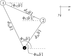
Figure 2: With GLI, the nodes obtain noisy observations of the relative orientation of each other with respect to the x-axis.

TABLE II: Nodes’ Observations

	No GLI	Perfect GLI
$o_{1}[i]$	$[\hat{d}_{1}[i]]$	$[\hat{d}_{1}[i],\hat{\phi}_{1}[i],l_{1}[i]]$
$o_{2}[i]$	$[\hat{d}_{2}[i]]$	$[\hat{d}_{2}[i],\hat{\phi}_{2}[i],l_{2}[i]]$
$o_{e}[i]$	$[\hat{d}_{1e}[i],\hat{d}_{2e}[i],\hat{\phi}_{e}[i]]$	$[\hat{d}_{1e}[i],\hat{d}_{2e}[i],\hat{\phi}_{1e}[i],\hat{\phi}_{2e}[i],l_{e}[i]]$

II-C Attacker Model

We assume that there exists a passive eavesdropper $e$, which does not transmit any beacons. However, node $e$ can strategically change its location to obtain a geographical advantage against the legitimate nodes. Overall, we consider two strategies:
Random Mobility: Eavesdropper moves randomly, without a regard to the location of the legitimate nodes. We will assume that eavesdropper adopts random mobility unless otherwise stated.
Mobile Man in the Middle: Node $e$ controls its mobility, such that it can move accordingly to obtain a geographic advantage compared to legitimate nodes. We consider the strategy where node $e$ moves to the mid-point of its maximum likelihood estimates of the legitimate nodes’ locations. For $j\in\{1,2\}$, let us denote node $e$’s maximum likelihood estimate of node $j$’s location at slot $i$, based on its observations up to slot $i-1$ as $\tilde{l}_{j,e}[i]$. Then,

$$\tilde{l}_{j,e}[i]=\arg\max_{l_{j}[i]\in{\cal L}}{\mathbb{P}}(l_{j}[i]|o_{e}[1],\ldots,o_{e}[i-1])$$

In other words, node $1$ and node $2$’s locations at slot $i$ is predicated by node $e$ by its observations in the previous slots. Then, at the beginning of each slot $i$, node $e$ moves to the mid-point of the estimates, which is $(\tilde{l}_{1,e}[i]+\tilde{l}_{2,e}[i])/2$.

Although we restricted ourselves to a single passive eavesdropper, we also discuss the implications of multiple eavesdroppers. The eavesdroppers may utilize their observations in two possible ways: (i) Non-colluding eavesdroppers do not communicate, or share their observations with each other, whereas (ii) colluding eavesdroppers combine their measurements to obtain less noisy measurements. Note that, an eavesdropper with multiple location sensors (e.g., multiple antennas in the case of wireless radio-based localization) is a special case of colluding eavesdroppers, as each sensor could be viewed as a separate eavesdropper, with perfect links between them. Theoretical secret key capacity under colluding eavesdropper scenario is lower, due to cooperation of the eavesdroppers, as discussed in Section III.

II-D Notion of security

We consider the typical definition of source model of information theoretic secrecy under a passive eavesdropper: We assume that there exists an authenticated error-free public channel, using which the legitimate nodes can communicate to agree on secret keys, based on the observations of the distances and angles (${\bf o}_{1}$ and ${\bf o}_{2}$) obtained during beacon exchange. This process, commonly referred to as public discussion [1], is a $T$ step message exchange protocol, where at any step $t\in\{1,\cdots,T\}$, node $1$ sends message $C_{1}[t]$, and node $2$ replies back with message $C_{2}[t]$ such that, for $t>1$,

$$H\big{(}C_{1}[t]|{{\bf o}}_{1},\{C_{1}[i]\}_{i=1}^{t-1},\{C_{2}[i]\}_{i=1}^{t-1}\big{)} =0,\mbox{ odd }t$$ (1)

$$H\big{(}C_{2}[t]|{{\bf o}}_{2},\{C_{1}[i]\}_{i=1}^{t},\{C_{2}[i]\}_{i=1}^{t-1}\big{)} =0,\mbox{ even }t.$$ (2)

At the end of the $T$ step protocol, node $1$ obtains ${\bf k}_{1}$, and node $2$ obtains ${\bf k}_{2}$ as the secret key, where

$$H\left({\bf k}_{j}|{{\bf o}}_{j},\{C_{1}[t],C_{2}[t]\}_{t=1}^{T}\right) =0,~{}j\in\{1,2\}.$$ (3)

Definition 1

Secret key bits are generated (with respect to the described attacker model) at rate $R$, if, for all $\epsilon>0$ and $\delta>0$, there exists some $n,\ T>0$ such that (1), (2) and (3) are satisfied, and

$$H({\bf k}_{j})/n =R,~{}j\in\{1,2\}$$ (4)

$${\mathbb{P}}({\bf k}_{1}\neq{\bf k}_{2}) \leq\epsilon$$ (5)

$$I({\bf k}_{j};{{\bf o}}_{e},\{C_{1}[t],C_{2}[t]\}_{t=1}^{T})/n \leq\delta,~{}j\in\{1,2\}.$$ (6)

Here, (4)-(6) correspond to perfect randomness, reliability and security constraints, respectively. The schemes proposed in the literature typically use a random coding structure, where $\{C_{1}[t],C_{2}[t]\}_{t=1}^{T}$ are generated by using a binning strategy [1]-[6]. In Section III, we will make use of these existing results to provide computable theoretical bounds on the achievable key rates.

III Theoretical Performance Limits

In this section, we provide information theoretical bounds on the achievable key rate with perfect reliability. To evaluate these bounds, we assume an idealized system by ignoring the issues associated with quantization, cascade reconciliation protocol, and privacy amplification. Thus, these bounds are valid for any key generation scheme that satisfies Definition 1.

Theorem 1

A lower bound $R_{L}$, and an upper bound $R_{U}$ on the perfectly-reliable key rate achievable through public discussion are

$$R_{L}=\max\bigg{\{}\lim_{n\to\infty}\frac{1}{n}\left[I({{\bf o}}_{1};{{\bf o}}_{2})-I({{\bf o}}_{1};{\bf o}_{e})\right]^{+},$$

$$\qquad\lim_{n\to\infty}\frac{1}{n}\left[I({\bf o}_{2};{\bf o}_{1})-I({\bf o}_{2};{{\bf o}}_{e})\right]^{+}\bigg{\}}$$ (7)

$$R_{U}=\lim_{n\to\infty}\frac{1}{n}\min\left\{I({\bf o}_{1};{\bf o}_{2}),I({\bf o}_{1};{\bf o}_{2}|{\bf o}_{e})\right\}$$ (8)

respectively, where ${\bf o}_{1},{\bf o}_{2}$ and ${\bf o}_{e}$ are as given in Table II for different possibilities of GLI.

The theorem follows from Theorem 4 in [18], which generalizes Maurer’s results on secret key generation through public discussion [1], to non-i.i.d. settings. Although tighter bounds exist in the literature [2, 3], we use the above bounds since they provide clearer insights into our systems due to their simplicity.

Note that for the special case where the observations $(o_{1}[i],o_{2}[i],o_{e}[i])$ are i.i.d., we can safely drop the index $i$, and denote the joint probability density function of observations as $f(o_{1},o_{2},o_{e})$. Therefore, the conditioning on the past and future observations in $R_{L}$ and $R_{U}$ disappear, and the bounds reduce to

$$R_{L}= \max\bigg{(}\left[I(o_{1};o_{2})-I(o_{1};o_{e})\right]^{+},$$

$$\left[I(o_{1};o_{2})-I(o_{2};o_{e})\right]^{+}\bigg{)}$$ (9)

$$R_{U}= \min\left(I(o_{1};o_{2}),I(o_{1};o_{2}|o_{e})\right),$$ (10)

Also note that Theorem 1 can be extended to provide key rate bounds against multiple eavesdropper models discussed in Section II-C. Consider $K$ eavesdroppers, with observations ${\bf o}_{e,1},\ldots,{\bf o}_{e,K}$. For the non-colluding eavesdroppers model, since the eavesdroppers are not communicating, we can safely consider the most capable eavesdropper $k$. In other words, in (7), (8) we can replace ${\bf o}_{e}$ with ${\bf o}_{e,k}$ for $k\in\{1,\ldots K\}$ which yields the lowest bounds, and discard the rest of the eavesdroppers. For the colluding eavesdroppers model, we can replace the term ${\bf o}_{e}$ in (7), (8) with ${\bf o}_{e,1},\ldots,{\bf o}_{e,K}$ since the eavesdroppers perfectly communicate with each other. It can be directly observed that the bounds for colluding case are lower with respect to the non-colluding case.

IV Gaussian observations

To obtain more insights from theoretical results in Section III, we focus on the following special case: First, we assume that the node locations are individually Markov processes such that

$$l_{j}[i-1]\rightarrow l_{j}[i]\rightarrow l_{j}[i+1],~{}j\in\{1,2,e\},$$

holds for any $i$, and their joint probability density function $f({\bf l}_{1},{\bf l}_{2},{\bf l}_{e})$ is well defined. Secondly, all observations of distance and angle terms are i.i.d. Gaussian processes. This model is typically used in the literature to characterize observation noise [19, 8]. To that end, for no GLI, $j\in\{1,2\}$

$$\hat{d}_{j}[i] =d_{12}[i]+w_{j}[i],~{}w_{j}[i]\raise 0.73193pt\hbox{$\scriptstyle\sim$}{\cal N}\left(0,\frac{\gamma(d_{12}[i])\rho_{j}}{P}\right)$$ (11)

$$\hat{d}_{je}[i] =d_{je}[i]+w_{je}[i],~{}w_{je}[i]\raise 0.73193pt\hbox{$\scriptstyle\sim$}{\cal N}\left(0,\frac{\gamma(d_{je}[i])\rho_{e}}{P}\right)$$ (12)

$$\hat{\phi}_{e}[i] =\phi_{e}[i]+w_{\phi_{e}}[i],~{}w_{\phi}[i]\raise 0.73193pt\hbox{$\scriptstyle\sim$}{\cal N}\left(0,\frac{\gamma_{\phi}(d_{1e}[i],d_{2e}[i])\rho_{e}}{P}\right)$$ (13)

are Gaussian noise processes, where $P$ is the beacon power. The observation noise variances are increasing functions of the distance, which are modeled by the increasing functions $\gamma$ for distance observations and $\gamma_{\phi}$ for angle observations. The parameter $\rho_{j}$ depends on the capability of the nodes. For instance, in wireless localization, $\gamma$ and $\gamma_{\phi}$ depend on the path loss exponent, and $\rho$ depends on receiver antenna gain, number of antennas, etc [19, 8]. For perfect GLI, we additionally assume that for $j\in\{1,2\}$,

$$\hat{\phi}_{j}[i] ={\phi}_{j}[i]+w_{\phi_{j}}[i],~{}w_{\phi_{j}}[i]\raise 0.73193pt\hbox{$\scriptstyle\sim$}{\cal N}\left(0,\frac{\gamma_{\phi}(d_{12}[i])\rho_{j}}{P}\right)$$ (14)

$$\hat{\phi}_{je}[i] ={\phi}_{je}[i]+w_{{\phi}_{je}}[i],~{}w_{{\phi}_{je}}[i]\raise 0.73193pt\hbox{$\scriptstyle\sim$}{\cal N}\left(0,\frac{\gamma_{\phi}(d_{je}[i])\rho_{e}}{P}\right)$$ (15)

Clearly, the achievable key rates depend highly on the functions $\gamma$, $\gamma_{\phi}$ and $\rho$. Note that, there there may be a bias on these observations due to small scale fading [19]. The effect of biased observations are studied in Appendix B.

IV-A Beacon Power Asymptotics

In this part, we analyze the beacon power asymptotics of the system. We show that, if the eavesdropper does not observe the angle, i.e., $\hat{\phi}_{e}=\emptyset$, then $R_{L}$ increases unboundedly with the beacon power $P$, which indicates that arbitrarily large secret key rates can be obtained. However, when eavesdropper observes the angle information, then $R_{U}$ remains bounded, which indicates that the advantage gained by increasing beacon power is rather limited. To clearly illustrate our insights, we present our results for the no GLI scenario. However, the same conclusion holds for the perfect GLI case as well.

Theorem 2

When the eavesdropper obtains angle information, i.e., $I(\hat{\hbox{\boldmath$\phi$}}_{e};\hbox{\boldmath$\phi$}_{e})>0$,

$$\lim_{P\to\infty}R_{U}<\infty.$$ (16)

The proof is in Appendix A, where we show that $\lim_{P\to\infty}R_{U}\leq\eta$, where

$$\eta =\frac{1}{2}\log\bigg{\{}2\pi{\mathbb{E}}\bigg{[}\frac{\rho_{e}}{d_{12}^{2}}\bigg{(}\frac{d_{12}^{2}\rho_{1}}{\rho_{e}}\gamma(d_{12})$$

$$+4(d_{1e}+d_{2e})^{2}(\sqrt{\gamma(d_{1e})}+\sqrt{\gamma(d_{2e})})^{2}$$

$$+(4d_{1e}d_{2e}+64(d_{1e}d_{2e})^{2})\gamma_{\phi}(d_{1e},d_{2e})$$

$$+8(d_{1e}+d_{2e})d_{1e}d_{2e}\big{(}\sqrt{\gamma(d_{1e})}$$

$$+\sqrt{\gamma(d_{2e})}\big{)}\sqrt{\gamma_{\phi}(d_{1e},d_{2e})}$$

$$+64(d_{1e}+d_{2e})^{2}(\gamma(d_{1e})+\gamma(d_{2e}))\bigg{)}\bigg{]}\bigg{\}}$$

$$-\frac{1}{2}{\mathbb{E}}\bigg{[}\log\left(2\pi\rho_{1}\gamma(d_{12})\right)\bigg{]}.$$ (17)

The parameter $\eta$ remains finite since the distances take on values in some bounded range $[d_{\min},d_{\max}]$ with probability $1$. Therefore, the secret key rate remains bounded.

Theorem 3

When the eavesdropper does not obtain any angle information, i.e., $I(\hat{\hbox{\boldmath$\phi$}}_{e};\hbox{\boldmath$\phi$}_{e})=0$,

$$\lim_{P\to\infty}\frac{R_{L}}{\frac{1}{2}\log(P)}=\lim_{P\to\infty}\frac{R_{U}}{\frac{1}{2}\log(P)}=1.$$

The proof is provided in Appendix A. Theorem 3 implies that, without the angle observation at the eavesdropper, an arbitrarily large key rate can be achieved with sufficiently large beacon power $P$. However, the key rate increases with $\log(P)$, which means that increasing the beacon power would provide diminishing returns.

IV-B Numerical Evaluations

We evaluate the theoretical bounds in Section III for Gaussian observations model, using Monte Carlo simulations.

Setup

We consider a simple $(M\times M)$ discrete 2-D grid, which simulates a city with $M$ blocks that covers a square field of area $A^{2}$, such that for any $j\in\{1,2,e\}$, $i\in\{1,\ldots,n\}$, $l_{j}[i]=[x~{}y]\in\{\frac{A}{M},\ldots,M\frac{A}{M}\}\times\{\frac{A}{M},\ldots,M\frac{A}{M}\}$. Node mobilities are Markov, and characterized by parameter $B$, where

$${\mathbb{P}}\big{(}l_{j}[i]=[x~{}y]~{}|~{} l_{j}[i-1]=[x^{\prime}~{}y^{\prime}]\big{)}=$$

$$\begin{cases}\frac{1}{(B+1)^{2}}\mbox{ if}&|x-x^{\prime}|\leq\frac{AB}{M}\\ &|y-y^{\prime}|\leq\frac{AB}{M}\\ ~{}~{}0&\mbox{ otherwise }\end{cases}$$

For no GLI, we choose $\gamma(d)=0.1+d^{2}$, and

$$\gamma_{\phi}(d_{1e},d_{2e})=\pi-\frac{\pi}{1.1+(d_{1e}^{2}+d_{2e}^{2})},$$

and for perfect GLI, we choose

$$\gamma_{\phi}(d_{je})=\pi-\frac{\pi}{1.1+\left(d_{je}\right)^{2}}$$

such that both parameters are strictly increasing functions of the distances. We consider node capability parameters $\rho_{1}=\rho_{2}=\rho_{e}=1$, unless stated otherwise. The theoretical key rates in Section III converge as $n\to\infty$, therefore they are calculated for large enough $n$, using the forward algorithm procedure.

Results

Due to computational limitations, we consider examples in which $M\leq 11$, and $B\leq 3$. Note that this choice limits the maximum achievable secret key rate.

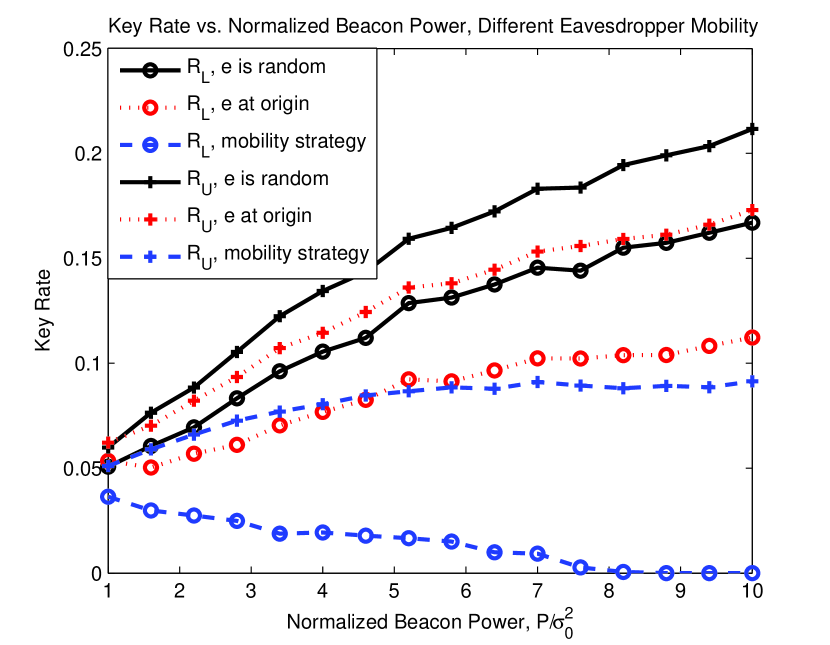
Figure 3: Effect of eavesdropper mobility on the key rate

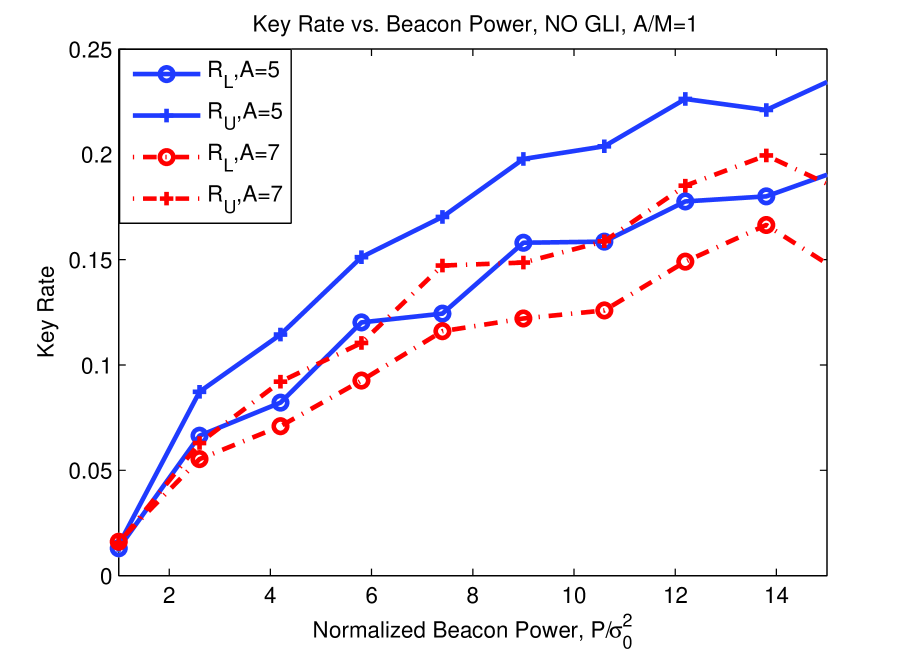
Figure 4: Bounds for no GLI vs normalized beacon power, for different $M$, $B=1$, $A/M=1$

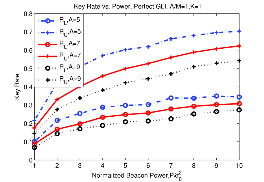
Figure 5: Bounds for perfect GLI vs normalized beacon power, for different $M$, $B=1$, $A/M=1$

Then, we analyze the effect of the different grid size, field area and GLI on the theoretical key rates. In Figures 5 and 5, we plot the bounds on the achievable key rate with respect to the normalized beacon power $P/\sigma_{0}^{2}$ for different grid size $M$ for no GLI and perfect GLI cases, respectively. We assumed a constant ratio of field size and grid size, $A/M=1$, and considered $B=1$. We can see that, there is a diminishing return on the increased power levels for the achievable key rate. Furthermore, we can see that increasing the field area $A^{2}$ has a negative impact on the key rate despite the increase in $M$, which is due to the fact that the common information of the legitimate nodes decreases as a result of increase in their observation error variance. Next, in Figures 6 and 7, we plot the bounds with respect to beacon power $P$, for different step size $B=1$ for no GLI and perfect GLI cases, respectively. We assumed $M=5$ for the no GLI case, and $M=7$ for perfect GLI case, and in both cases, the ratio of field size and grid size is constant, such that $A/M=1$. We can clearly see the positive effect of the increased step size on the secret key rate. This is due to the increase in different distance combinations that are possible.

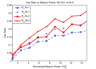
Figure 6: Upper and lower bounds for no GLI vs normalized beacon power $P/\sigma_{0}^{2}$, $M=A=5$, for different $B$

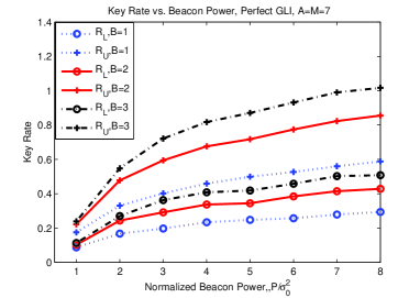
Figure 7: Upper and lower bounds for perfect GLI vs normalized beacon power $P/\sigma_{0}^{2}$, $M=A=7$, for different $B$

Finally, we analyze the effect of eavesdropper mobility on the achievable key rate. In Figure 5, for $M=7$, $A=5$ and $B=1$, we plot the secret key rate bounds versus beacon power for the cases where the eavesdropper i) follows the random mobility pattern described in the setup with parameter $B=1$, ii) stays at the origin, and iii) follows the man in the middle strategy described in Section II-C, i.e., moves to the mid point of its location estimates of nodes $1$ and $2$. We can see that, compared to following a random mobility pattern, the eavesdropper can reduce the achievable secret key rate significantly by following this strategy. However, the rate still remains positive. We observe that the eavesdropper can also reduce the key rate by simply staying static at a certain favorable location, rather than moving randomly. However, in practice this may not be feasible for the eavesdropper, since by staying put, it will lose connection completely with the legitimate nodes in a large region.

V Conclusion

In this paper, we showed that relative localization information is an additional resource for generating secret key bits in mobile networks. We studied the information theoretic limits of secret key generation, and characterized lower and upper bounds of key rates utilizing results for the cases in which the nodes are/are not capable of observing their global locations. Focusing on the special case where the observation noise is i.i.d. Gaussian, we studied the beacon power asymptotics, and observed that, interestingly, when the eavesdropper cannot observe the angle information, the secret key rate grows unboundedly. The following research directions can be further investigated 1) theoretical performance analysis of secret key generation in large networks, taking into account the recent advances in network information theoretic security, and 2) security analysis of various adversarial models, such as active jamming attacks, or impersonation attacks in unauthenticated networks.

Appendix A Proofs of Theorems in Section IV-A

A-A Proof of Theorem 2

We first provide three lemmas that will be useful when proving the theorem.

Lemma 1

Let $x$ and $y$ be random variables. Then,

$${\mathbb{V}ar}(x+y) \leq 2{\mathbb{V}ar}(x)+2{\mathbb{V}ar}(y).$$ (18)

If $x$ and $y$ are independent, then ${\mathbb{V}ar}(x+y)={\mathbb{V}ar}(x)+{\mathbb{V}ar}(y)$.

Proof:

When $x$ and $y$ are not independent,

$${\mathbb{V}ar}(x+y) ={\mathbb{V}ar}(x)+{\mathbb{V}ar}(y)+2{\mathbb{C}ov}(x,y)$$

$$\leq{\mathbb{V}ar}(x)+{\mathbb{V}ar}(y)+2\sqrt{{\mathbb{V}ar}(x){\mathbb{V}ar}(y)}$$

$$\leq 2{\mathbb{V}ar}(x)+2{\mathbb{V}ar}(y).$$ (19)

where (19) follows from the fact that ${\mathbb{V}ar}(x)+{\mathbb{V}ar}(y)\geq 2\sqrt{{\mathbb{V}ar}(x){\mathbb{V}ar}(y)}$. When $x$ and $y$ are independent, ${\mathbb{C}ov}(x,y)=0$, implying the result. $\Box$

Lemma 2

Let $x$ be a random variable such that ${\mathbb{E}}[x]\geq\mu$, where $\mu>-1$. Let $\alpha=\frac{\sqrt{1+\mu}}{1+\mu}$. Then, ${\mathbb{V}ar}(\sqrt{[1+x]^{+}})\leq{\mathbb{V}ar}(\alpha x)$.

Proof:

Assume ${\mathbb{E}}[x]=\mu^{\prime}$, where $\mu^{\prime}\geq\mu$. Let $\alpha^{\prime}=\frac{\sqrt{1+\mu^{\prime}}}{1+\mu^{\prime}}$. Let us define $f_{1}(x)\triangleq\sqrt{[1+x]^{+}}$, and $f_{2}(x)\triangleq\alpha^{\prime}(1+x)$. Note that,

$${\mathbb{V}ar}(\sqrt{[1+x]^{+}})={\mathbb{V}ar}(f_{1}(x))\leq{\mathbb{E}}\big{[}(f_{1}(x)-{\mathbb{E}}[f_{2}(x)])^{2}\big{]}$$

since the centralized second moment is minimized around the mean. Also,

$${\mathbb{V}ar}(\alpha x)\geq{\mathbb{V}ar}(\alpha^{\prime}x)={\mathbb{V}ar}(f_{2}(x))$$

since $\mu^{\prime}\geq\mu$, and $\alpha^{\prime}\leq\alpha$. Therefore, it suffices to show that $\forall x$,

$$|f_{1}(x)-{\mathbb{E}}[f_{2}(x)]| \leq|f_{2}(x)-{\mathbb{E}}[f_{2}(x)]|$$ (20)

$$=|f_{2}(x)-\sqrt{1+\mu^{\prime}}|.$$ (21)

i) First note that $f_{1}(\mu^{\prime})=f_{2}(\mu^{\prime})=\sqrt{1+\mu^{\prime}}$. Therefore, the condition (21) is satisfied for $x=\mu^{\prime}$.
ii) For $x>\mu^{\prime}$,

$$f_{1}(x) \leq f_{1}(\mu^{\prime})+f_{1}^{\prime}(\mu^{\prime})(x-\mu^{\prime})$$ (22)

$$\leq\sqrt{1+\mu^{\prime}}+\alpha(x-\mu^{\prime})=f_{2}(x)$$

where $f_{1}^{\prime}(\mu^{\prime})$ is the first derivative of $f_{1}(x)$ at point $x=\mu^{\prime}$. (22) follows from the fact that $f_{1}(x)$ is a strictly concave function in the interval $[-1~{}\infty)$. Therefore, condition (21) is satisfied for $x>\mu^{\prime}$.
iii) Combining the facts that $f_{1}(x)$ is a strictly concave function of $x$ in the interval $[-1~{}\infty)$; $f_{2}(x)$ is linear; $f_{1}(-1)=f_{2}(-1)$; and $f_{1}(\mu^{\prime})=f_{2}(\mu^{\prime})$, we can see that $\sqrt{1+\mu^{\prime}}>f_{1}(x)\geq f_{2}(x)$ when $-1<x<\mu^{\prime}$. Therefore, condition (21) is satisfied for $-1<x<\mu^{\prime}$. iv) When $x<-1$, $f_{1}(x)=0$ and $f_{2}(x)<0$, therefore, condition (21) is satisfied. This concludes the proof. $\Box$

Lemma 3

Let $x$, $y$ be random variables. Then,

$${\mathbb{V}ar}\left({\mathbb{E}}\left[1-\sqrt{(1+x)^{+}}~{}\big{|}y\right]\right)\leq{\mathbb{E}}\left[\big{(}{\mathbb{E}}\big{[}~{}|x|~{}\big{|}~{}y\big{]}\big{)}^{2}\right].$$

Proof:

Note that

$${\mathbb{V}ar}\left({\mathbb{E}}\left[1-\sqrt{(1+x)^{+}}~{}\big{|}y\right]\right)$$

$$\quad\leq{\mathbb{E}}\left[{\mathbb{E}}\left[1-\sqrt{(1+x)^{+}}~{}\big{|}y\right]^{2}\right].$$

Since for any $x$, $|1-\sqrt{(1+x)^{+}}|\leq|x|$,

$$\bigg{|}{\mathbb{E}}\left[1-\sqrt{(1+x)^{+}}~{}\big{|}y\right]\bigg{|}\leq{\mathbb{E}}\big{[}~{}|x|~{}\big{|}~{}y\big{]}$$

is satisfied for any $y$, which completes the proof. $\Box$

Now, we proceed as follows. Assume without loss of generality that $\rho_{\min}=\min(\rho_{1},\rho_{2})=\rho_{1}$. When $\hat{\hbox{\boldmath$\phi$}}_{e}\neq\emptyset$,

$$R_{U}= \lim_{n\to\infty}\frac{1}{n}I(\hat{{\bf d}}_{1};\hat{{\bf d}}_{2}|\hat{{\bf d}}_{1e},\hat{{\bf d}}_{2e},\hat{\hbox{\boldmath$\phi$}}_{e})$$

$$\leq \lim_{n\to\infty}\frac{1}{n}\big{(}h(\hat{{\bf d}}_{1}|\hat{{\bf d}}_{1e},\hat{{\bf d}}_{2e},\hat{\hbox{\boldmath$\phi$}}_{e})-h(\hat{{\bf d}}_{1}|{\bf d}_{12})\big{)}$$ (23)

$$\leq \lim_{n\to\infty}\frac{1}{n}\sum_{i=1}^{n}\bigg{(}h(\hat{d}_{1}[i]|\hat{d}_{1e}[i],\hat{d}_{2e}[i],\hat{\phi}_{e}[i])-$$

$$h(\hat{d}_{1}[i]-d_{12}[i]|d_{12}[i])\bigg{)}$$

$$= h(\hat{d}_{1}|\hat{d}_{1e},\hat{d}_{1e},\hat{\phi}_{e})-h(\hat{d}_{1}-d_{12}|d_{12})$$ (24)

where (23) follows from the fact that $\hat{{\bf d}}_{1}\rightarrow{\bf d}_{12}\rightarrow(\hat{{\bf d}}_{2},\hat{{\bf d}}_{1e},\hat{{\bf d}}_{2e},\hat{\hbox{\boldmath$\phi$}}_{e})$ forms a Markov chain, and (24) follows from the fact that all of the random variables $\hat{d}_{1}[i],\hat{d}_{1e}[i],\hat{d}_{2e}[i],\hat{\phi}_{e}[i]$ have a stationary distribution, denoted as $\hat{d}_{1},\hat{d}_{1e},\hat{d}_{2e}$ and $\hat{\phi}_{e}$, respectively. The second term in (24) can be found as

$$h(\hat{d}_{1}-d_{12}|d_{12})=\frac{1}{2}{\mathbb{E}}\left[\log\left(\frac{\gamma(d_{12})\rho_{1}}{P}\right)\right]$$ (25)

from the definition of $\hat{d}_{1}[i]$. Now, we bound the first term in (24). Let us define

$$\hat{d}_{e}\triangleq\sqrt{[\hat{d}_{1e}^{2}+\hat{d}_{2e}^{2}-2\hat{d}_{1e}\hat{d}_{2e}\cos(\hat{\phi}_{e})]^{+}}.$$

Then,

$$h(\hat{d}_{1}|\hat{d}_{1e},\hat{d}_{2e},\hat{\phi}_{e}) \leq h\big{(}\hat{d}_{1}|\hat{d}_{e}\big{)}\leq h\big{(}\hat{d}_{1}-\hat{d}_{e}\big{)}.$$ (26)

Note that for a given variance, Gaussian distribution maximizes the entropy. Therefore, the entropy of a Gaussian random variable that has a variance identical to that of $\hat{d}_{1}-\hat{d}_{e}$ will be an upper bound for (26). We proceed as follows.

$${\mathbb{V}ar}\big{(}\hat{d}_{1}-\hat{d}_{e}\big{)}= {\mathbb{E}}\big{[}{\mathbb{V}ar}\big{(}\hat{d}_{1}-\hat{d}_{e}|d_{12},d_{1e},d_{2e}\big{)}\big{]}$$

$$+{\mathbb{V}ar}\big{(}{\mathbb{E}}\big{[}\hat{d}_{1}-\hat{d}_{e}|d_{12},d_{1e},d_{2e}\big{]}\big{)},$$ (27)

where (27) follows from the fact that for any dependent random variables $x$ and $y$, ${\mathbb{V}ar}(x)={\mathbb{E}}[{\mathbb{V}ar}(x|y)]+{\mathbb{V}ar}({\mathbb{E}}[x|y])$. We now find an upper bound on the first term of (27). Note that,

$${\mathbb{V}ar}\big{(}\hat{d}_{1}-\hat{d}_{e}|d_{12},d_{1e},d_{2e}\big{)}= {\mathbb{V}ar}(\hat{d}_{1}|d_{12})$$

$$+{\mathbb{V}ar}\big{(}\hat{d}_{e}|d_{12},d_{1e},d_{2e}\big{)}$$ (28)

due to Lemma 1, since $\hat{d}_{1}\rightarrow(d_{12},d_{1e},d_{2e})\rightarrow(\hat{d}_{1e},\hat{d}_{2e},\hat{\phi}_{e})\rightarrow\hat{d}_{e}$ forms a Markov chain, and the fact that $\hat{d}_{1}$ is independent of ${d}_{1e},d_{2e}$ given $d_{12}$. The first term in (28) is equal to

$${\mathbb{V}ar}(\hat{d}_{1}|d_{12})={\mathbb{V}ar}\big{(}w_{1}|d_{12}\big{)}=\frac{\gamma(d_{12})\rho_{1}}{P}.$$ (29)

We bound the second term in (28) as follows. Let us define

$$\kappa \triangleq\frac{1}{d_{12}^{2}}\bigg{(}2(d_{1e}-d_{2e}\cos(\hat{\phi_{e}}))w_{1e}+{w_{1e}}^{2}$$

$$~{}+{w_{2e}}^{2}+2(d_{2e}-d_{1e}\cos(\hat{\phi}_{e}))w_{2e}$$

$$~{}+2d_{1e}d_{2e}(\cos(\phi_{e})-\cos(\hat{\phi}_{e}))-2{w_{1e}}{w_{2e}}\cos(\hat{\phi}_{e})\bigg{)}.$$

Then,

$$\quad{\mathbb{V}ar}(\hat{d}_{e}|d_{12},d_{1e},d_{2e})$$

$$={\mathbb{V}ar}\bigg{\{}\bigg{(}\bigg{[}d_{1e}^{2}+d_{2e}^{2}+2(d_{1e}-d_{2e}\cos\hat{\phi_{e}})w_{1e}+$$

$$~{}2(d_{2e}-d_{1e}\cos\hat{\phi}_{e})w_{2e}-2d_{1e}d_{2e}\cos\hat{\phi}_{e}+{w_{1e}}^{2}$$

$$~{}+{w_{2e}}^{2}-2{w_{1e}}{w_{2e}}\cos\hat{\phi}_{e}\bigg{]}^{+}\bigg{)}^{0.5}|d_{12},d_{1e},d_{2e}\bigg{\}}$$ (30)

$$\leq d_{12}^{2}{\mathbb{V}ar}(\sqrt{[1+\kappa]^{+}}),$$ (31)

where (30) follows due to the definitions of $\hat{d}_{1e}$, $\hat{d}_{2e}$ and $\hat{\phi}_{e}$. (31) follows due to definition of $\kappa$, and the cosine law $d_{12}^{2}=d_{1e}^{2}+d_{2e}^{2}-2d_{1e}d_{2e}\cos(\phi_{e})$. Now we will apply Lemma 2 to bound (31). First, note that

$${\mathbb{E}}[\kappa]=\frac{1}{d_{12}^{2}}{\mathbb{E}}\bigg{[}w_{1e}^{2}+w_{2e}^{2}-2d_{1e}d_{2e}(\cos\phi_{e}-\cos\hat{\phi}_{e})\bigg{]}$$

$$\geq\frac{1}{Pd_{12}^{2}}{\mathbb{E}}\bigg{[}w_{1e}^{2}+w_{2e}^{2}-2d_{1e}d_{2e}|w_{\phi_{e}}|\bigg{]}$$

$$\geq\frac{\rho_{e}}{Pd_{12}^{2}}{\mathbb{E}}\bigg{[}\gamma(d_{1e})+\gamma(d_{2e})-2d_{1e}d_{2e}\sqrt{\frac{2P\gamma_{\phi}(d_{1e},d_{2e})}{\pi\rho_{e}}}\bigg{]},$$ (32)

where (32) follows from the fact that since $w_{\phi_{e}}$ is zero mean Gaussian, $|w_{\phi_{e}}|$ follows a Half-normal distribution with ${\mathbb{E}}(|w_{\phi_{e}}|)=\sqrt{\frac{2\gamma_{\phi}(d_{1e},d_{2e})\rho_{e}}{P\pi}}$. We can choose $P_{1}$ such that for any beacon power $P>P_{1}$, ${\mathbb{E}}[x]>-\frac{3}{4}$. Let $\mu=-\frac{3}{4}$, and $\alpha=\frac{\sqrt{1+\mu}}{1+\mu}=2$. Due to Lemma 2, we obtain

$$d_{12}^{2} {\mathbb{V}ar}(\sqrt{[1+\kappa]^{+}})\leq d_{12}^{2}{\mathbb{V}ar}(\alpha\kappa)$$

$$\leq \frac{4\alpha^{2}}{d_{12}^{2}}\bigg{(}{\mathbb{V}ar}(2(d_{1e}-d_{2e}\cos(\hat{\phi_{e}}))w_{1e})$$ (33)

$$+{\mathbb{V}ar}(2(d_{2e}-d_{1e}\cos(\hat{\phi}_{e}))w_{2e})$$

$$+{\mathbb{V}ar}(2d_{1e}d_{2e}(\cos(\phi_{e})-\cos(\hat{\phi}_{e})))$$

$$+{\mathbb{V}ar}(2{w_{1e}}{w_{2e}}\cos(\hat{\phi}_{e}))+{\mathbb{V}ar}(w_{1e}^{2})+{\mathbb{V}ar}(w_{2e}^{2})\bigg{)}$$

$$\leq {\mathbb{E}}\bigg{[}\frac{16\rho_{e}}{Pd_{12}^{2}}\bigg{(}4(d_{1e}+d_{2e})^{2}(\gamma(d_{1e})+\gamma(d_{2e}))$$ (34)

$$+4(d_{1e}d_{2e})^{2}\gamma_{\phi}(d_{1e},d_{2e})+o\left(\frac{1}{P}\right)\bigg{)}\bigg{]},$$ (35)

where (33) follows from applying Lemma 1 to ${\mathbb{V}ar}(\kappa)$ twice, and (35) follows from the fact that

$${\mathbb{V}ar}(2(d_{ie}-d_{je}\cos(\hat{\phi}_{e}))w_{ie})\leq{\mathbb{V}ar}(2(d_{ie}+d_{je})w_{ie})$$

for $i,j\in\{1,2\}$, and

$${\mathbb{V}ar} (2d_{1e}d_{2e}(\cos(\phi_{e})-\cos(\hat{\phi}_{e})))$$

$$={\mathbb{V}ar}(2d_{1e}d_{2e}(\cos(\phi_{e})-\cos(\phi_{e}+w_{\phi}))$$

$$\leq{\mathbb{V}ar}(2d_{1e}d_{2e}w_{\phi}).$$

Now, we upper bound the second term of (27) as

$${\mathbb{V}ar}\big{(}{\mathbb{E}}\big{[}\hat{d}_{1}-\hat{d}_{e}|d_{12},d_{1e},d_{2e}\big{]}\big{)}$$

$$={\mathbb{V}ar}\bigg{(}d_{12}{\mathbb{E}}\bigg{[}1-\sqrt{\left(1+\kappa\right)^{+}}|d_{12},d_{1e},d_{2e}\bigg{]}\bigg{)}$$ (36)

$$\leq{\mathbb{E}}\left[d_{12}^{2}\left({\mathbb{E}}\big{[}|x|~{}|d_{12},d_{1e},d_{2e}\big{]}\right)^{2}\right]$$ (37)

$$\leq{\mathbb{E}}\bigg{[}\frac{1}{d_{12}^{2}}{\mathbb{E}}\big{[}2(d_{1e}+d_{2e})(|w_{1e}|+|w_{2e}|)+w_{1e}^{2}+w_{2e}^{2}$$

$$+2d_{1e}d_{2e}|w_{\phi_{e}}|+2|w_{1e}w_{2e}|~{}|d_{12},d_{1e},d_{2e}\big{]}^{2}\bigg{]}$$

$$={\mathbb{E}}\bigg{[}\frac{\rho_{e}^{2}}{Pd_{12}^{2}}\bigg{(}2(d_{1e}+d_{2e})\frac{\sqrt{\gamma(d_{1e})}+\sqrt{\gamma(d_{2e})}}{\sqrt{\rho_{e}}}$$

$$+2d_{1e}d_{2e}\gamma_{\phi}(d_{1e},d_{2e})$$

$$+\frac{\gamma(d_{1e})+\gamma(d_{2e})}{\sqrt{P}}+2\frac{\sqrt{\gamma(d_{1e})+\gamma(d_{2e})}}{\sqrt{P\rho_{e}}}\bigg{)}^{2}\bigg{]}$$ (38)

$$={\mathbb{E}}\bigg{[}\frac{\rho_{e}^{2}}{Pd_{12}^{2}}\bigg{(}\frac{4(d_{1e}+d_{2e})^{2}}{\rho_{e}}(\sqrt{\gamma(d_{1e})}+\sqrt{\gamma(d_{2e})})^{2}$$

$$+4(d_{1e}d_{2e}\gamma_{\phi}(d_{1e},d_{2e}))^{2}$$

$$+\frac{8(d_{1e}+d_{2e})d_{1e}d_{2e}}{\rho_{e}}\big{(}\sqrt{\gamma(d_{1e})}$$

$$\quad+\sqrt{\gamma(d_{2e})}\big{)}\sqrt{\gamma_{\phi}(d_{1e},d_{2e})}\bigg{)}\bigg{]}+o(1/P).$$ (39)

where (36) follows from the fact that $\hat{d}_{e}=d_{12}\sqrt{(1+\kappa)^{+}}$, and (37) follows from Lemma 3. Finally, we obtain

$$R_{U} \leq h(\hat{d}_{1}-\hat{d}_{e})-h(\hat{d}_{1}-d_{12}|d_{12})$$ (40)

$$\leq\frac{1}{2}\log\left(2\pi{\mathbb{V}ar}(\hat{d}_{1}-\hat{d}_{e})\right)-h(w_{1}|d_{12})$$ (41)

$$=\frac{1}{2}\log\bigg{\{}2\pi{\mathbb{E}}\bigg{[}\frac{\rho_{e}}{d_{12}^{2}P}\bigg{(}\frac{d_{12}^{2}\rho_{1}}{\rho_{e}}\gamma(d_{12})$$

$$+4(d_{1e}+d_{2e})^{2}(\sqrt{\gamma(d_{1e})}+\sqrt{\gamma(d_{2e})})^{2}$$

$$+(4d_{1e}d_{2e}+64(d_{1e}d_{2e})^{2})\gamma_{\phi}(d_{1e},d_{2e})$$

$$+8(d_{1e}+d_{2e})d_{1e}d_{2e}\big{(}\sqrt{\gamma(d_{1e})}$$

$$+\sqrt{\gamma(d_{2e})}\big{)}\sqrt{\gamma_{\phi}(d_{1e},d_{2e})}$$

$$+64(d_{1e}+d_{2e})^{2}(\gamma(d_{1e})+\gamma(d_{2e}))\bigg{)}+o\left(\frac{1}{P}\right)\bigg{]}\bigg{\}}$$

$$-\frac{1}{2}{\mathbb{E}}\bigg{[}\log\left(\frac{2\pi\rho_{1}\gamma(d_{12})}{P}\right)\bigg{]},$$ (42)

where (40) follows from (24) and (26), (41) follows from the fact that entropy of $\hat{d}_{1}-\hat{d}_{e}$ is upper bounded by the entropy of a Gaussian random variable that has the same variance as $\hat{d}_{1}-\hat{d}_{e}$. The first term of (42) is obtained by combining combining (29), (35) and (39), and the second term of (42) follows from (25). As $P\to\infty$, the $P$ terms in (42) cancel each other since for any random variables $u$ and $v$,

$$\lim_{P\to\infty}\log{\mathbb{E}}\left[\frac{u}{P}+o\bigg{(}\frac{1}{P}\bigg{)}\right]-{\mathbb{E}}\left[\log\frac{v}{P}\right]=\log{\mathbb{E}}[u]-{\mathbb{E}}[\log v]$$

hence $\lim_{P\to\infty}R_{U}<\infty$.

A-B Proof of Theorem 3

When the eavesdropper does not observe the angle, $\hat{\hbox{\boldmath$\phi$}}_{e}=\emptyset$. Hence

$$R_{L}=\lim_{n\to\infty}\frac{1}{n}\left(h(\hat{{\bf d}}_{1}|\hat{{\bf d}}_{1e},\hat{{\bf d}}_{2e})-h(\hat{{\bf d}}_{1}|\hat{{\bf d}}_{2})\right)$$ (43)

First, we show that the first term in (43) is finite.

$$\lim_{P,n\to\infty}\frac{1}{n}h(\hat{{\bf d}}_{1}|\hat{{\bf d}}_{1e},\hat{{\bf d}}_{2e})=\lim_{n\to\infty}\frac{1}{n}h({\bf d}_{12}|{\bf d}_{1e},{\bf d}_{2e})$$

$$=\lim_{n\to\infty}\frac{1}{n}\sum_{i=1}^{n}h(d_{12}[i]|{\bf d}_{1e},{\bf d}_{2e},\{d_{12}[j]\}_{j=1}^{i-1})$$

$$=\lim_{n\to\infty}\frac{1}{n}\sum_{i=1}^{n}h(d_{12}[i]|{\bf d}_{1e},{\bf d}_{2e},\{\phi_{e}[j]\}_{j=1}^{i-1})$$ (44)

$$=\lim_{n\to\infty}\frac{1}{n}\sum_{i=1}^{n}h\bigg{(}\big{(}d_{1e}[i]^{2}+d_{2e}[i]^{2}-$$

$$2d_{1e}[i]d_{2e}[i]\cos(\phi_{e}[i])\big{)}^{0.5}|{\bf d}_{1e},{\bf d}_{2e},\{\phi_{e}[j]\}_{j=1}^{i-1}\bigg{)}>-\infty$$ (45)

where (44) follows from the fact that a triangle is completely characterized by either three sides $(d_{12}[i]\,d_{1e}[i],d_{2e}[i])$, or two sides and an angle $(d_{12}[i]\,d_{1e}[i],\phi_{e}[i])$. Equation (45) follow from the cosine law. Since the probability density function of $\hbox{\boldmath$\phi$}_{e},{\bf d}_{12}$ and ${\bf d}_{1e},{\bf d}_{2e}$ are well defined, we can see that $h(\phi_{e}[i]|{\bf d}_{1e},{\bf d}_{2e},\{\phi_{e}[j]\}_{j=1}^{i-1})>-\infty$. The second term

$$\frac{1}{n}h(\hat{{\bf d}}_{1}|\hat{{\bf d}}_{2}) \leq\frac{1}{n}h(\hat{{\bf d}}_{1}-\hat{{\bf d}}_{2})=h(w_{1}-w_{2})$$ (46)

$$\leq\frac{1}{2}\log\left(2\pi{\mathbb{E}}\left[\frac{4\rho_{\max}\gamma(d_{12})}{P}\right]\right)$$ (47)

$$=\frac{1}{2}\log\big{(}2\pi{\mathbb{E}}\left[4\rho_{\max}\gamma(d_{12})\right]\big{)}-\frac{1}{2}\log(P).$$

where (46) follows due to the fact that conditioning reduces entropy, (47) follows from the fact $\hat{d}_{1}[i]-\hat{d}_{2}[i]=w_{1}[i]-w_{2}[i]$ for any $i$. Dropping the index $i$, we can see that $h(w_{1}-w_{2})$ is upper bounded by entropy of a Gaussian random variable that has the same variance as $w_{1}-w_{2}$, which is

$${\mathbb{V}ar}(w_{1}-w_{2}) ={\mathbb{V}ar}({\mathbb{E}}[w_{1}-w_{2}])+{\mathbb{E}}({\mathbb{V}ar}[w_{1}-w_{2}])$$

$$={\mathbb{E}}_{d_{12}}({\mathbb{V}ar}[w_{1}-w_{2}])\leq{\mathbb{E}}\left[\frac{4\rho_{\max}\gamma(d_{12})}{P}\right].$$

Therefore, we can see that $\lim_{P\to\infty}\frac{R_{L}}{\frac{1}{2}\log(P)}\geq 1$ Now, we find an upper bound on $R_{U}$. Note that

$$R_{U}= \lim_{n\to\infty}\frac{1}{n}I(\hat{{\bf d}}_{1};\hat{{\bf d}}_{2}|\hat{{\bf d}}_{1e},\hat{{\bf d}}_{2e})$$

$$\leq \lim_{n\to\infty}\frac{1}{n}\big{(}h(\hat{{\bf d}}_{1}|\hat{{\bf d}}_{1e},\hat{{\bf d}}_{2e})-h(\hat{{\bf d}}_{1}|{\bf d}_{12})$$ (48)

where the first term of (48) is finite. The second term can be upper bounded as

$$\frac{1}{n}h(\hat{{\bf d}}_{1}|{{\bf d}}_{12}) =h(w_{1}|d_{12})$$

$$\geq{\mathbb{E}}\left[\frac{1}{2}\log\left(\frac{2\pi\rho_{1}\gamma(d_{12})}{P}\right)\right]$$

$$=\frac{1}{2}{\mathbb{E}}\left[\log\left(2\pi\rho_{1}\gamma(d_{12})\right)\right]-\frac{1}{2}\log(P),$$

therefore $\lim_{P\to\infty}\frac{R_{U}}{\frac{1}{2}\log(P)}\leq 1$. Since $R_{L}\leq R_{U}$ by definition, the proof is complete.

Appendix B On Observation Bias

Nodes’ observations may have bias due to several factors. We consider two different source of bias; clock mismatch and multipath fading. We will see that different types of bias may have different outcomes. In this part, we present our results for no GLI. However, the conclusions are valid for perfect GLI as well.

B-A Clock Mismatch

Assume that there is a clock mismatch between nodes $1$, and $2$. Consequently, all the observations of $d_{12}$ of nodes $1$ and $2$ in localization phase are shifted by a random value $\eta_{1}$ and $\eta_{2}$ respectively:

$$\hat{d}_{j}[i]=d_{12}[i]+w_{j}[i]+\eta_{j}$$ (49)

for $j\in\{1,2\}$, where $w_{j}[i]$ is as given in (11). We assume the amount of clock mismatch is a non-random, but unknown parameter, which remains constant througout the entire session. Since $w_{j}[i]$, $j\in\{1,2\}$ are zero mean random variables,

$${\mathbb{E}}[\hat{d}_{j}[i]|\eta_{1},\eta_{2}]={\mathbb{E}}[d_{12}[i]]+\eta_{j}.$$ (50)

Hence, with the knowledge of the statistics of the mobility, each node $j\in\{1,2\}$ can obtain a perfect estimate of the amount of clock mismatch $\eta_{j}$ as $n\to\infty$, by simply calculating the difference between the long-term average of the distance observations $\hat{d}_{j}[i]$ for all $i$ and the known mean distance ${\mathbb{E}}[d_{12}]$. Then this value can be broadcast in the public discussion phase. Therefore, clock mismatch does not affect the theoretical bounds of secret key generation rates.

B-B Multipath Fading

There may be a bias in the observations when the nodes experience multipath fading. An example of this is time of arrival observation of distances when the nodes are not within their line of sight. Note that, this kind of bias does not remain constant, and varies from one slot to the other. The impact of fading can be viewed as that of an additional observation noise source and the distance observations can be written as

$$\hat{d}_{j}[i]=d_{12}[i]+w_{j}[i]+\eta_{j}[i]$$

for $j\in\{1,2\}$.

Consequently, one will observe a reduction in the key rate. For example, with no angle observation at the eavesdropper, we know from Section IV-A that the key rate grows unboundedly with the beacon power $P$. However, with multipath fading, independent over different locations,

$$\lim_{P\to\infty}h(\hat{{\bf d}}_{1}|\hat{{\bf d}}_{2}) =h(\hbox{\boldmath$\eta$}_{1}|\hbox{\boldmath$\eta$}_{2})$$

$$\stackrel{{\scriptstyle(a)}}{{=}}h(\hbox{\boldmath$\eta$}_{1})>-\infty,\vspace{-0.1in}$$

where $\hbox{\boldmath$\eta$}_{1}=\{\eta_{1}[i]\}_{i=1}^{n}$, and $(a)$ follows since $\hbox{\boldmath$\eta$}_{1}$ and $\hbox{\boldmath$\eta$}_{2}$ are independent. Hence, following an identical approach to Section IV-A, one see that $\lim_{P\to\infty}R_{L}<\infty$, i.e., the secret key rate remains bounded even as the power grows unboundedly.

References

• [1] U. M. Maurer, “Secret key agreement by public discussion from common information,” IEEE Trans. Information Theory, vol.39, no.3, pp.733-742, May 1993
• [2] R. Ahlswede and I. Csiszar, “Common randomness in information theory and cryptography. I. Secret sharing,” IEEE Trans. Information Theory , vol.39, no.4, pp.1121-1132, Jul 1993
• [3] U. M. Maurer and S. Wolf, “Unconditionally secure key agreement and the intrinsic conditional information,” IEEE Trans. Information Theory , vol.45, no.2, pp.499-514, Mar 1999
• [4] I. Csiszar and P. Narayan, “Secrecy capacities for multiterminal channel models,” IEEE Trans. Information Theory, vol.54, no.6, pp.2437-2452, June 2008
• [5] U. M. Maurer and S. Wolf, “Secret-key agreement over unauthenticated public channels .I. Definitions and a completeness result,” IEEE Transactions on Information Theory, vol.49, no.4, pp. 822- 831, April 2003
• [6] I. Csiszar and P. Narayan, “Common randomness and secret key generation with a helper,” IEEE Transactions on Information Theory, vol.46, no.2, pp.344-366, Mar 2000
• [7] U. M. Maurer, and S. Wolf, “Information-theoretic key agreement: From weak to strong secrecy for free,” Advances in Cryptology EUROCRYPT 2000, Springer Berlin Heidelberg, 2000.
• [8] S. Gezici, Z. Tian, G. B. Giannakis, H. Kobayashi, A.F. Molisch, H.V. Poor, and Z. Sahinoglu, “Localization via ultra-wideband radios: a look at positioning aspects for future sensor networks,” IEEE Signal Processing Magazine, vol.22, no.4, pp. 70- 84, July 2005
• [9] Y. Shen and M.Z. Win,“Fundamental limits of wideband localization Part I: A general framework,” IEEE Trans. Information Theory, vol.56, no.10, pp.4956-4980, Oct. 2010
• [10] H. Buhrman, N. Chandran, V. Goyal, R. Ostrovsky and C. Schaffner, “Position-based quantum cryptography: Impossibility and constructions,”, 2010
• [11] A. Srivinasan and J. Vu, “A survey on secure localization in wireless sensor networks”, Encyclopedia of Wireless and Mobile Communications, 2007
• [12] R. Poovendran, C. Wang, S. Roy, “Secure localization and time synchronization for wireless sensor and ad-hoc networks”, Springer Verlag, 2007
• [13] N. Chandran, V. Goyal, R. Moriarty and R. Ostrovsky, “Position based cryptography,” Cryptology ePrint Archive, 2009, http://eprint.iacr.org/2009/
• [14] Wilson, R.; Tse, D.; Scholtz, R.A.; , “Channel identification: Secret sharing using reciprocity in ultrawideband channels,” IEEE International Conf. Ultra-Wideband, ICUWB 2007, pp.270-275, 24-26 Sept. 2007
• [15] Kirchner, Nathan, and Tomonari Furukawa, “Infrared localisation for indoor uavs,” ICST05: Proceedings of the 2005 International Conference on Sensing Technology, 2005.
• [16] Jim nez, A. R., and F. Seco, “Ultrasonic localization methods for accurate positioning,” Instituto de Automatica Industrial, Madrid (2005).
• [17] S. Verdu and T. S. Han, “A general formula for channel capacity,” IEEE Transactions on Information Theory, vol.40, no.4, pp.1147-1157, Jul 1994
• [18] M. R. Bloch and J. N. Laneman, “Secrecy from resolvability,” arXiv:1105.5419 [cs.IT], May 2011
• [19] D. Jourdan, D. Dardari and M. Win, “Position error bound for UWB localization in dense cluttered environments,” IEEE Transactions on Aerospace and Electronic Systems, vol.44, no.2, pp.613-628, April 2008
• [20] S. Mathur, W. Trappe, N. Mandayam, C. Ye and A. Reznik, “Radio-telepathy: extracting a secret key from an unauthenticated wireless channel,” Proceedings of the 14th ACM international conference on Mobile computing and networking (MobiCom ’08) ACM, New York, NY, USA, 128-139
• [21] S. Jana, S. N. Premnath, M. Clark, S. K. Kasera, N. Patwari and S. V. Krishnamurthy, “On the effectiveness of secret key extraction from wireless signal strength in real environments,” Proceedings of the 15th annual international conference on Mobile computing and networking (MobiCom ’09) ACM, New York, NY, USA, 321-332
• [22] J. Zhang, S.K. Kasera and N. Patwari, “Mobility assisted secret key generation using wireless link signatures,” Proc. IEEE INFOCOM 2010, vol., no., pp.1-5, 14-19 March 2010
• [23] N. Patwari, J. Croft, S. Jana and S. K. Kasera, “High-rate uncorrelated bit extraction for shared secret key generation from channel measurements,” IEEE Transactions on Mobile Computing , vol.9, no.1, pp.17-30, Jan. 2010
• [24] C. Ye, S. Mathur, A. Reznik, Y. Shah, W. Trappe, and N. B. Mandayam, “Information-theoretically secret key generation for fading wireless channels,” IEEE Transactions on Information Forensics and Security, no. 2 (2010): 240-254.
• [25] S. Banerjee and A. Mishra, “Secure spaces: Location-based secure group communication for wireless networks,” ACM MobiCom, vol. 7, pp. 68 70, Sep. 2002.
• [26] A. Pierrot, R. Chou and M. Bloch, “Practical Limitations of Secret-Key Generation in Narrowband Wireless Environments,” arXiv:1312.3304 [cs.IT], Dec. 2012
• [27] S. Mathur, R. Miller, A. Varshavsky, W. Trappe, and N. Mandayam, ‘Proximate: Proximity-based secure pairing using ambient wireless signals,” ACM MobiSys, pp. 211 224, Jun. 2011.
• [28] NIST, “A statistical test suite for the validation of random number generators and pseudo random number generators for cryptographic applications,” 2001
• [29] G.Brassard and L. Salvail, “Secret-key reconciliation by public discussion,” in Workshop on the theory and application of cryptographic techniques on Advances in cryptology (EUROCRYPT ’93), Tor Helleseth (Ed.). Springer-Verlag New York, Inc., Secaucus, NJ, USA, 410-423.
• [30] https://code.google.com/p/miniz/
• [31] O. S. Oguejiofor, V. N. Okorogu and OBO Adewale Abe, “Outdoor localization system using RSSI measurement of wireless sensor network”
• [32] D. Klinc, H. Jeongseok, S.W. McLaughlin, J. Barros and K. Byung-Jae, “LDPC Codes for the gaussian wiretap channel,” IEEE Transactions on Information Forensics and Security, vol.6, no.3, pp.532,540, Sept. 2011
• [33] O. Gungor, F. Chen; Koksal, C.E., “Secret key generation from mobility,” Proc. IEEE 2011 GLOBECOM Workshop on Physical Layer Security, pp.874,878, 5-9 Dec. 2011