Measuring Tie Strength in Implicit Social Networks

Abstract

Given a set of people and a set of events they attend, we address the problem of measuring connectedness or tie strength between each pair of persons given that attendance at mutual events gives an implicit social network between people. We take an axiomatic approach to this problem. Starting from a list of axioms that a measure of tie strength must satisfy, we characterize functions that satisfy all the axioms and show that there is a range of measures that satisfy this characterization. A measure of tie strength induces a ranking on the edges (and on the set of neighbors for every person). We show that for applications where the ranking, and not the absolute value of the tie strength, is the important thing about the measure, the axioms are equivalent to a natural partial order. Also, to settle on a particular measure, we must make a non-obvious decision about extending this partial order to a total order, and that this decision is best left to particular applications. We classify measures found in prior literature according to the axioms that they satisfy. In our experiments, we measure tie strength and the coverage of our axioms in several datasets. Also, for each dataset, we bound the maximum Kendall’s Tau divergence (which measures the number of pairwise disagreements between two lists) between all measures that satisfy the axioms using the partial order. This informs us if particular datasets are well behaved where we do not have to worry about which measure to choose, or we have to be careful about the exact choice of measure we make.

1 Introduction

Explicitly declared friendship links suffer from a low signal to noise ratio (e.g. Facebook friends or LinkedIn contacts). Links are added for a variety of reasons like reciprocation, peer-pressure, etc. Detecting which of these links are important is a challenge.

Social structures are implied by various interactions between users of a network. We look at event information, where users participate in mutual events. Our goal is to infer the strength of ties between various users given this event information. Hence, these social networks are implicit.

There has been a surge of interest in implicit social networks. We can see anecdotal evidence for this in startups like COLOR (http://www.color.com) and new features in products like Gmail. COLOR builds an implicit social network based on people’s proximity information while taking photos. Gmail’s don’t forget bob Roth et al. (2010) feature uses an implicit social network to suggest new people to add to an email given a existing list.

People attend different events with each other. In fact, an event is defined by the set of people that attend it. An event can represent the set of people who took a photo at the same place and time, like COLOR, or a set of people who are on an email, like in Gmail. Given the set of events, we would like to infer how connected two people are, i.e. we would like to measure the strength of the tie between people. All that is known about each event is the list of people who attended it. People attend events based on an implicit social network with ties between pairs of people. We want to solve the inference problem of finding this weighted social network that gives rise to the set of events.

Given a bipartite graph, with people as one set of vertices and events as the other set, we want to infer the tie-strength between the set of people. Hence, in our problem, we do not even have access to any directly declared social network between people, in fact, the social network is implicit. We want to infer the network based on the set of people who interact together at different points in time.

We start with a set of axioms and find a characterization of functions that could serve as a measure of tie strength, just given the event information. We do not end up with a single function that works best under all circumstances, and in fact we show that there are non-obvious decisions that need to be made to settle down on a single measure of tie strength.

Moreover, we examine the case where the absolute value of the tie strength is not important, just the order is important (see Section 4.2.1). We show that in this case the axioms are equivalent to a natural partial order on the strength of ties. We also show that choosing a particular tie strength function is equivalent to choosing a particular linear extension of this partial order.

Our contributions are:

• We present an axiomatic approach to the problem of inferring implicit social networks by measuring tie strength.

• We characterize functions that satisfy all the axioms and show a range of measures that satisfy this characterization.

• We show that in ranking applications, the axioms are equivalent to a natural partial order; we demonstrate that to settle on a particular measure, we must make non-obvious decisions about extending this partial order to a total order which is best left to the particular application.

• We classify measures found in prior literature according to the axioms that they satisfy.

• In our experiments, we show that by using Kendall’s Tau divergence, we can judge whether a dataset is well-behaved, where we do not have to worry about which tie-strength measure to choose, or we have to be careful about the exact choice of measure.

The remainder of this paper is structured as follows. Section 2 outlines the related work. Section 3 presents our proposed model. Sections 4 and 5 describe the axioms and measures of tie strength, respectively. Section 6 presents our experiments. Section 7 concludes the paper.

2 Related Work

(Granovetter, 1973) introduced the notion of strength of ties in social networks and since then has affected different areas of study. We split the related works into different subsections that emphasize particular methods/applications.

Strength of Ties: (Granovetter, 1973) showed that weak ties are important for various aspects like spread of information in social networks. There have been various studies on identifying the strength of ties given different features of a graph. (Gilbert and Karahalios, 2009) model tie strength as a linear combination of node attributes like intensity, intimacy, etc to classify ties in a social network as strong or weak. The weights on each attribute enable them to find attributes that are most useful in making these predictions. (Kahanda and Neville, 2009) take a supervised learning approach to the problem by constructing a predictor that determines whether a link in a social network is a strong tie or a weak tie. They report that network transactional features, which combine network structure with transactional features like the number of wall posting, photos, etc like $\frac{|posts(i,j)|}{\Sigma_{k}|posts_{(}j,k)|}$, form the best predictors.

Link Prediction: (Adamic and Adar, 2003) considers the problem of predicting links between web-pages of individuals, using information such as membership of mailing lists and use of common phrases on web pages. They define a measure of similarity between users by creating a bipartite graph of users on the left and features (e.g., phrases and mailing-lists) on the right as $w(u,v)=\sum_{(i\text{ neighbor of }u\&v)}\frac{1}{\log|i|}$. (Liben-Nowell and Kleinberg, 2003) formalizes the problem of predicting which new interactions will occur in a social network given a snapshot of the current state of the network. It uses many existing predictors of similarity between nodes like (Adamic and Adar, 2003; Jeh and Widom, 2002; Katz, 1953) and generates a ranking of pairs of nodes that are currently not connected by an edge. It compares across different datasets to measure the efficacy of these measures. Its main finding is that there is enough information in the network structure that all the predictors handily beat the random predictor, but not enough that the absolute number of predictions is high. (Allali, Magnien, and Latapy, 2011) addresses the problem of predicting links in a bipartite network. They define internal links as links between left nodes that have a right node in common, i.e. they are at a distance two from each other and the predictions that are offered are only for internal links.

Email networks: Because of the ubiquitous nature of email, there has been a lot of work on various aspects of email networks. (Roth, Ben-David, Deutscher, Flysher, Horn, Leichtberg, Leiser, Matias, and Merom, 2010) discusses a way to suggest more recipients for an email given the sender and the current set of recipients. This feature has been integrated in the Google’s popular Gmail service. (Kahanda and Neville, 2009) constructs a regression model for classifying edges in a social network as strong or weak. They achieve high accuracy and find that network-transactional features like number of posts from $u$ to $v$ normalized by the total number of posts by $u$ achieve the largest gain in accuracy of prediction.

Axiomatic approach to Similarity: (Altman and Tennenholtz, 2005) were one of the first to axiomatize graph measures. In particular, they studied axiomatizing PageRank. The closest in spirit to our work is the work by Lin (Lin, 1998) that defines an information theoretic measure of similarity. This measure depends on the existence of a probability distribution on the features that define objects. While the measure of tie strength between people is similar to a measure of similarity, there are important differences. We do not have any probability distribution over events, just a log of the ones that occurred. More importantly, (Lin, 1998) defines items by the attributes or features they have. Hence, items with the same features are identical. In our case, even if two people attend all the same events, they are not the same person, and in fact they might not even have very high tie strength depending on how large the events were.

3 Model

We model people and events as nodes and use a bipartite graph $G=(L\cup R,E)$ where the edges represent membership. The left vertices correspond to people while the right vertices correspond to events. We ignore any information other than the set of people who attended the events, like the timing, location, importance of events. These are features that would be important to the overall goal of measuring tie strength between users, but in this work we focus on the task of inferring tie strength using the graph structure only. We shall denote users in $L$ by small letters ($u,v,\ldots$) and events in $R$ by capital letters($P,Q,\ldots$). There is an edge between $u$ and $P$ if and only if $u$ attended event $P$. Hence, our problem is to find a function on bipartite graphs that models tie strength between people, given this bipartite graph representation of events.

Figure 1: Given a bipartite person $\times$ event graph, we want to infer the induced partial order of tie strength among the people.

We also introduce some notation. We shall denote the tie strength of $u$ and $v$ due to a graph $G$ as $TS_{G}(u,v)$ or as $TS(u,v)$ if $G$ is obvious from context. We shall also use $TS_{\{E_{1},\ldots,E_{k}\}}(u,v)$ to denote the tie strength between $u$ and $v$ in the graph induced by events ${\{E_{1},\ldots,E_{k}\}}$ and users that attend at least one of these events. For a single event $E$, then $TS_{E}(u,v)$ denotes the tie strength between $u$ and $v$ if $E$ where the only event.

We denote the set of natural numbers by $\mathbb{N}$. A sequence of $k$ natural numbers is given by $(a_{1},\ldots,a_{k})$ and the set of all such sequences is $\mathbb{N}^{k}$. The set of all finite sequence of natural numbers is represented as $\mathbb{N}^{*}=\cup_{k}\mathbb{N}^{k}$

4 Axioms of Tie Strength

We now discuss the axioms that measures of tie strength between two users $u$ and $v$ must follow.

Axiom 1 (Isomorphism)

Suppose we have two graphs $G$ and $H$ and a mapping of vertices such that $G$ and $H$ are isomorphic. Let vertex $u$ of $G$ map to vertex $a$ of $H$ and vertex $v$ to $b$. Then $TS_{G}(u,v)=TS_{H}(a,b)$. Hence, the tie strength between $u$ and $v$ does not depend on the labels of $u$ and $v$, only on the link structure.

Axiom 2 (Baseline)

If there are no events, then the tie strength between each pair $u$ and $v$ is 0. $TS_{\phi}(u,v)=0$. If there are only two people $u$ and $v$ and a single party which they attend, then their tie strength is $1$. $TS_{\{u,v\}}(u,v)=1$.

Axiom 3 (Frequency: More events create stronger ties)

All other things being equal, the more events common to $u$ and $v$, the stronger the tie strength of $u$ and $v$.
Given a graph $G=(L\cup R,E)$ and two vertices $u,v\in L$. Consider the graph $G^{\prime}=(L\cup(R\cup P),E\cup P_{u,v,\ldots})$, where $P_{u,v,\ldots}$ is a new event which both $u$ and $v$ attend. Then the $TS_{G^{\prime}}(u,v)\geq TS_{G}(u,v)$.

Axiom 4 (Intimacy: Smaller events create stronger ties)

All other things being equal, the fewer invitees there are to any particular party attended by $u$ and $v$, the stronger the tie strength between $u$ and $v$.
Given a graph $G=(L\cup R,E)$ such that $P\in R$ and $(P,u),(P,v),(P,w)\in E$ for some vertex $w$. Consider the graph $G^{\prime}=(L\cup R),E-(P,w))$, where the edge $(P,w)$ is deleted. Then the $TS_{G}(u,v)\geq TS_{G^{\prime}}(u,v)$.

Axiom 5 (Larger events create more ties)

Consider two events $P$ and $Q$. If the number of people attending $P$ is larger than the number of people attending $Q$, then the total tie strength created by event $P$ is more than that created by event $Q$.
$|P|\geq|Q|\implies\sum_{u,v\in P}TS_{P}(u,v)\geq\sum_{u,v\in Q}TS_{Q}(u,v)$.

Axiom 6 (Conditional Independence of Vertices)

The tie strength of a vertex $u$ to other vertices does not depend on events that $u$ does not attend; it only depends on events that $u$ attends.

Axiom 7 (Conditional Independence of Events)

The increase in tie strength between $u$ and $v$ due to an event $P$ does not depend other events, just on the existing tie strength between $u$ and $v$.
$TS_{G+P}(u,v)=g(TS_{G}(u,v),TS_{P}(u,v))$ for some fixed function monotonically increasing function $g$.

Axiom 8 (Submodularity)

The marginal increase in tie strength of $u$ and $v$ due to an event $Q$ is at most the tie strength between $u$ and $v$ if $Q$ was their only event.
If $G$ is a graph and $Q$ is a single event, $TS_{G}(u,v)+TS_{Q}(u,v)\geq TS_{G+Q}(u,v)$.

Discussion

These axioms give a measure of tie strength between nodes that is positive but unbounded. Nodes that have a higher value are closer to each other than nodes that have lower value.

We get a sense of the axioms by applying them to Figure 1. Axiom 1 (Isomorphism) implies that $TS(b,c)=TS(b,d)$ and $TS(c,e)=TS(d,e)$. Axiom 2 (Baseline), Axiom 6 (Conditional Independence of Vertices) and Axiom 7 (Conditional Independence of Events) imply that $TS(a,c)=TS(a,d)=TS(a,e)=TS(b,e)=0$. Axiom 4 (Intimacy: Smaller events create stronger ties) implies that $TS(a,b)\geq TS(d,e)$. Axiom 3 (Frequency: More events create stronger ties) implies that $TS(c,d)\geq TS(d,e)$.

While each of the axioms above are fairly intuitive, they are hardly trivial. In fact, we shall see that various measures used in prior literature break some of these axioms. On the other hand, it might seem that satisfying all the axioms is a fairly strict condition. However, we shall see that even satisfying all the axioms are not sufficient to uniquely identify a measure of tie strength. The axioms leave considerable space for different measures of tie strength.

One reason the axioms do not define a particular function is that there is inherent tension between Axiom 4 (Intimacy: Smaller events create stronger ties) and Axiom 3 (Frequency: More events create stronger ties). While both state ways in which tie strength becomes stronger, the axioms do not resolve which one dominates the other or how they interact with each other. This is a non-obvious decision that we feel is best left to the application in question. In Figure 1, we cannot tell using just Axioms (1-8)  which of $TS(a,b)$ and $TS(c,d)$ is larger. We discuss this more more in Section 4.2.

4.1 Characterizing Tie Strength

In this section, we shall state and prove Theorem 6 that gives a characterization of all functions that satisfy the axioms of tie strength. Axioms (1-8)  do not uniquely define a function, and in fact, one of the reasons that tie strength is not uniquely defined up to the given axioms is that we do not have any notion for comparing the relative importance of number of events (frequency) versus the exclusivity of events (intimacy). For example, in terms of the partial order, it is not clear whether $u$ and $v$ having in common two events with two people attending them is better than or worse than $u$ and $v$ having three events in common with three people attending them.

We shall use the following definition for deciding how much total tie strength a single event generates, given the size of the event.

Notation 1.

If there is a single event, with $k$ people, we shall denote the total tie-strength generated as $f(k)$.

Lemma 2 (Local Neighborhood).

The tie strength of $u$ and $v$ is affected only by events that both $u$ and $v$ attend.

Proof.

Given a graph $G$ and users $u$ and $v$ in $G$, $G^{-u}$ is obtained by deleting all events that $u$ is not a part of. Similarly, $G^{-u,v}$ is obtained by deleting all events of $G^{-u}$ that $v$ is not a part of. By Axiom 6 (Conditional Independence of Vertices), tie strength of $u$ only depends on events that $u$ attends. Hence, $TS_{G}(u,v)=TS_{G^{-u}}(u,v)$. Also, tie strength of $v$ only depends on events that $v$ attends. Hence, $TS_{G}(u,v)=TS_{G^{-u}}(u,v)=TS_{G^{-u,v}}(u,v)$. This proves our claim. ∎

Lemma 3.

The tie strength between any two people is always non-negative and is equal to zero if they have never attended an event together.

Proof.

If two people have never attended an event together, then from Lemma 2 the tie strength remains unchanged if we delete all the events not containing either which in this case is all the events. Then Axiom 2 (Baseline) tells us that $TS(u,v)=0$.

Also, Axiom 3 (Frequency: More events create stronger ties) implies that $TS_{G}(u,v)\geq TS_{\phi}(u,v)=0$. Hence, the tie strength is always non-negative. ∎

Lemma 4.

If there is a single party, with $k$ people, the Tie Strength of each tie is equal to $\frac{f(k)}{{k\choose 2}}$.

Proof.

By Axiom 1 (Isomorphism), it follows that the tie-strength on each tie is the same. Since the sum of all the ties is equal to $f(k)$, and there are ${k\choose 2}$ edges, the tie-strength of each edge is equal to $\frac{f(k)}{{k\choose 2}}$. ∎

Lemma 5.

The total tie strength created at an event $E$ with $k$ people is a monotone function $f(k)$ that is bounded by $1\leq f(k)\leq{k\choose 2}$

Proof.

By Axiom 4 (Intimacy: Smaller events create stronger ties) , the tie strength of $u$ and $v$ due to $E$ is less than that if they were alone at the event. $TS_{E}(u,v)\leq TS_{u,v}(u,v)=1$, by the Baseline axiom. Summing up over all ties gives us that $\sum_{u,v}TS_{E}(u,v)\leq{k\choose 2}$. Also, since larger events generate more ties, $f(k)\geq f(i):\forall i<k$. In particular, $f(k)\geq f(1)=1$. This proves the result. ∎

We are now ready to state the main theorem in this section.

Theorem 6.

Given a graph $G=(L\cup R,E)$ and two vertices $u,v$, if the tie-strength function $TS$ follows Axioms (1-8), then the function has to be of the form

$$TS_{G}(u,v)=g(h(|P_{1}|),h(|P_{2}|),\ldots,h(|P_{k}|))$$

where $\{P_{i}\}_{1\leq i\leq k}$ are the events common to both $u$ and $v$, $h:\mathbb{N}\to$ is a monotonically decreasing function bounded by $1\geq h(n)\geq\frac{1}{{n\choose 2}}$ and $g:\mathbb{N}^{*}\to$ is a monotonically increasing submodular function.

Proof.

Given two users $u$ and $v$ we use Axioms (1-8)  to successively change the form of $TS_{G}(u,v)$. Let $\{P_{i}\}_{1\leq i\leq k}$ be all the events common to $u$ and $v$. Axiom 7 (Conditional Independence of Events) implies that $TS_{G}(u,v)=g(TS_{P_{i}}(u,v))_{1\leq i\leq k}$, where $g$ is a monotonically increasing submodular function. Given an event $P$, $TS_{P}(u,v)=h(|P|)=\frac{f(|P|)}{{|P|\choose 2}}$. By Axiom 4 (Intimacy: Smaller events create stronger ties) , $h$ is a monotonically decreasing function. Also, by Lemma 5, $f$ is bounded by $1\leq f(n)\leq{n\choose 2}$. Hence, $h$ it bounded by $1\geq h(n)\geq\frac{1}{{n\choose 2}}$. This completes the proof of the theorem. ∎

Theorem 6 gives us a way to explore the space of valid functions for representing tie strength and find which work given particular applications. In Section 5 we shall look at popular measure of tie strength and show that most of them follow Axioms (1-8)  and hence are of the form described by Theorem 6. We also describe the functions $h$ and $g$ that characterize these common measures of tie strength . While Theorem 6 gives a characterization of functions suitable for describing tie strength, they leave open a wide variety of functions. In particular, it does not give the comfort of having a single function that we could use. We discuss the reasons for this and what we would need to do to settle upon a particular function in the next section.

4.2 Tie Strength and Orderings

We begin this section with a definition of order in a set.

Definition 7 (Total Order).

Given a set $S$ and a binary relation $\leq_{\mathcal{O}}$ on $S$, $\mathcal{O}=(S,\leq_{\mathcal{O}})$ is called a total order if and only if it satisfies the following properties (i Total). for every $u,v\in S$, $u\leq_{\mathcal{O}}v$ or $v\leq_{\mathcal{O}}u$ (ii Anti-Symmetric). $u\leq_{\mathcal{O}}v\text{ and }v\leq_{\mathcal{O}}u\implies u=v$ (iii Transitive). $u\leq_{\mathcal{O}}v$ and $v\leq_{\mathcal{O}}w\implies u\leq_{\mathcal{O}}w$

A total order is also called a linear order.

Consider a measure $TS$ that assigns a measure of tie strength to each pair of nodes $u,v$ given the events that all nodes attend in the form of a graph $G$. Since $TS$ assigns a real number to each edge and the set of reals is totally ordered, $TS$ gives a total order on all the edges. In fact, the function $TS$ actually gives a total ordering of $\mathbb{N}^{*}$. In particular, if we fix a vertex $u$, then $TS$ induces a total order on the set of neighbors of $u$, given by the increasing values of $TS$ on the corresponding edges.

4.2.1 The Partial Order on $\mathbb{N}^{*}$

Definition 8 (Partial Order).

Given a set $S$ and a binary relation $\leq_{\mathcal{P}}$ on $S$, $\mathcal{P}=(S,\leq_{\mathcal{P}})$ is called a partial order if and only if it satisfies the following properties (i Reflexive). for every $u\in S,u\leq_{\mathcal{P}}u$ (ii Anti-Symmetric). $u\leq_{\mathcal{P}}v\text{ and }v\leq_{\mathcal{P}}u\implies u=v$ (iii Transitive). $u\leq_{\mathcal{P}}v$ and $v\leq_{\mathcal{P}}w\implies u\leq_{\mathcal{P}}w$

The set $S$ is called a partially ordered set or a poset.

Note the difference from a total order is that in a partial order not every pair of elements is comparable. We shall now look at a natural partial order $\mathcal{N}=(\mathbb{N}^{*},\leq_{\mathcal{N}})$ on the set $\mathbb{N}^{*}$ of all finite sequences of natural numbers. Recall that $\mathbb{N}^{*}=\cup_{k}\mathbb{N}^{k}$. We shall think of this sequence as the number of common events that a pair of users attend.

Definition 9 (Partial order on $N^{*}$).

Let $a,b\in\mathbb{N}^{*}$ where $a=(a_{i})_{1\leq i\leq A}$ and $b=(b_{i})_{1\leq i\leq B}$. We say that $a\geq_{\mathcal{N}}b$ if and only if $A\geq B$ and $a_{i}\leq b_{i}:1\leq i\leq B$. This gives the partial order $\mathcal{N}=(\mathbb{N}^{*},\leq_{\mathcal{N}})$.

The partial order $\mathcal{N}$ corresponds to the intuition that more events and smaller events create stronger ties. In fact, we claim that this is exactly the partial order implied by the Axioms (1-8). Theorem 11 formalizes this intuition along with giving the proof. What we would really like is a total ordering. Can we go from the partial ordering given by the Axioms (1-8)  to a total order on $\mathbb{N}^{*}$? Theorem 11 also suggest ways in which we can do this.

4.2.2 Partial Orderings and Linear Extensions

In this section, we connect the definitions of partial order and the functions of tie strength that we are studying. First we start with a definition.

Definition 10 (Linear Extension).

$\mathcal{L}=(S,\leq_{\mathcal{L}})$ is called the linear extension of a given partial order $\mathcal{P}=(S,\leq_{\mathcal{P}})$ if and only if $\mathcal{L}$ is a total order and $\mathcal{L}$ is consistent with the ordering defined by $\mathcal{P}$, that is, for all $u,v\in S$, $u\leq_{\mathcal{P}}v\implies u\leq_{\mathcal{L}}v$.

We are now ready to state the main theorem which characterizes functions that satisfy Axioms (1-8)  in terms of a partial ordering on $\mathbb{N}^{*}$. Fix nodes $u$ and $v$ and let $P_{1},\ldots,P_{n}$ be all the events that both $u$ and $v$ attend. Consider the sequence of numbers $(|P_{i}|)_{1\leq i\leq k}$ that give the number of people in each of these events. Without loss of generality assume that these are sorted in ascending order. Hence $|P_{i}|\leq|P_{i+1}|$. We associate this sorted sequence of numbers with the tie $(u,v)$. The partial order $\mathcal{N}$ induces a partial order on the set of pairs via this mapping. We also call this partial order $\mathcal{N}$. Fixing any particular measure of tie strength, gives a mapping of $\mathbb{N}^{*}$ to and hence implies fixing a particular linear extension of $\mathcal{N}$, and fixing a linear extension of $\mathcal{N}$ involves making non-obvious decisions between elements of the partial order. We formalize this in the next theorem.

Theorem 11.

Let $G=(L\cup R,E)$ be a bipartite graph of users and events. Given two users $(u,v)\in(L\times L)$, let $(|P_{i}|)_{1\leq i\leq k}\in R$ be the set of events common to users $(u,v)$. Through this association, the partial order $\mathcal{N}=(\mathbb{N}^{*},\leq_{\mathcal{N}})$ on finite sequences of numbers induces a partial order on $L\times L$ which we also call $\mathcal{N}$.

Let $TS$ be a function that satisfies Axioms (1-8). Then $TS$ induces a total order on the edges that is a linear extension of the partial order $\mathcal{N}$ on $L\times L$.

Conversely, for every linear extension $\mathcal{L}$ of the partial order $\mathcal{N}$, we can find a function $TS$ that induces $\mathcal{L}$ on $L\times L$ and that satisfies Axioms (1-8).

Proof.

$TS:L\times L\to$. Hence, it gives a total order on the set of pairs of user. We want to show that if $TS$ satisfies Axioms (1-8), then the total order is a linear extension of $\mathcal{N}$. The characterization in Theorem 6 states that given a pair of vertices $(u,v)\in(L\times L)$, $TS(u,v)$ is characterized by the number of users in events common to $u$ and $v$ and can be expressed as $TS_{G}(u,v)=g(h(|P_{i}|))_{1\leq i\leq k}$ where $g$ is a monotone submodular function and $h$ is a monotone decreasing function. Since $TS:L\times L\to$, it induces a total order on all pairs of users. We now show that this is a consistent with the partial order $\mathcal{N}$. Consider two pairs $(u_{1},v_{1}),(u_{2},v_{2})$ with party profiles $a=(a_{1},\ldots,a_{A})$ and $b=(b_{1},\ldots,b_{B})$.

Suppose $a\geq_{\mathcal{N}}b$. We want to show that $TS(u_{1},v_{1})\geq TS(u_{2},v_{2})$. $a\geq_{\mathcal{N}}b$ implies that $A\geq B$ and that $a_{i}\leq b_{i}:\forall 1\leq i\leq B$.

$$TS(u_{1},v_{1})$$

$$=g(h(a_{1}),\ldots,h(a_{A}))$$

$$\geq g(h(a_{1}),\ldots,h(a_{B}))\text{ (Since $g$ is monotone and $A\geq B$) }$$

$$\geq g(h(b_{1}),\ldots,h(b_{B}))\text{ (Since $g$ is monotone and }$$

$$\qquad h(a_{i})\geq h(b_{i})\text{ since }a_{i}\leq b_{i})$$

$$=TS(u_{2},v_{2})$$

This proves the first part of the theorem.

For the converse, we are given an total ordering $\mathcal{L}=(\mathbb{N}^{*},\leq_{\mathcal{L}})$ that is an extension of the partial order $\mathcal{N}$. We want to prove that there exists a tie strength function $TS:L\times L\to$ that satisfies Axioms (1-6) and that induces $\mathcal{L}$ on $L\times L$. We shall prove this by constructing such a function. We shall define a function $f:\mathbb{N}^{*}\to\mathbb{Q}$ and define $TS_{G}(u,v)=f(a_{1},\ldots,a_{k})$, where $a_{i}=|P_{i}|$, the number of users that attend event $P_{i}$ in $G$.

Define $f(n)=\frac{1}{n-1}$ and $f(\phi)=0$. Hence, $TS_{\phi}(u,v)=f(\phi)=0$ and $TS_{\{u,v\}}(u,v)=f(2)=\frac{1}{2-1}=1$. This shows that $TS$ satisfies Axiom 2 (Baseline). Also, define $f(\underbrace{1,1,\ldots,1}_{n})=n$. Since $\mathbb{N}^{*}$ is countable, consider elements in some order. If for the current element $a$ under consideration, there exists an element $b$ such that $a=_{\mathcal{N}}b$ and we have already defined $TS(b)$, then define $TS(a)=TS(b)$. Else, find let $a_{glb}=argmax_{e}\left\{TS(e)\text{ is defined and }a\geq_{\mathcal{N}}e\right\}$ and let $a_{lub}=\operatorname{argmin}_{e}\left\{TS(e)\text{ is defined and }a\leq_{\mathcal{N}}e\right\}$. Since, at every point the sets over which we take the maximum of minimum are finite, both $a_{glb}$ and $a_{lub}$ are well defined and exist. Define $TS(a)=\frac{1}{2}\left(TS(a_{glb})+TS(a_{lub})\right)$. ∎

In this abstract framework, an intuitively appealing linear extension is the random linear extension of the partial order under consideration. There are polynomial time algorithms to calculate this (Karzanov and Khachiyan, 1991). We leave the analysis of the analytical properties and its viability as a strength function in real world applications as an open research question.

In the next section, we turn our attention to actual measures of tie strength. We see some popular measures that have been proposed before as well as some new ones.

5 Measures of tie strength

	Axiom 1 (Isomorphism)	Axiom 2 (Baseline)	Axiom 3 (Frequency: More events create stronger ties)	Axiom 4 (Intimacy: Smaller events create stronger ties)	Axiom 5 (Larger events create more ties)	Axiom 6 (Conditional Independence of Vertices)	Axiom 7 (Conditional Independence of Events)	Axiom 8 (Submodularity)	$g(a_{1},\ldots,a_{k})$ and $h(|P_{i}|)=a_{i}$ (From the characterization in Theorem 6)
Common Neighbors.	✓	✓	✓	✓	✓	✓	✓	✓	$g(a_{1},\ldots,a_{k})=\sum_{i=1}^{k}a_{i}\newline h(n)=1$
Jaccard Index.	✓	✓	✓	✓	✓	x	x	x	x
Delta.	✓	✓	✓	✓	✓	✓	✓	✓	$g(a_{1},\ldots,a_{k})=\sum_{i=1}^{k}a_{i}\newline h(n)=\frac{1}{{n\choose 2}}$
Adamic and Adar.	✓	✓	✓	✓	✓	✓	✓	✓	$g(a_{1},\ldots,a_{k})=\sum_{i=1}^{k}a_{i}\newline h(n)=\frac{1}{\log n}$
Katz Measure.	✓	x	✓	✓	✓	✓	x	x	x
Preferential attachment.	✓	✓	x	✓	✓	✓	x	x	x
Random Walk with Restarts.	✓	x	x	x	✓	✓	x	x	x
Simrank.	✓	x	x	x	x	x	x	x	x
Max.	✓	✓	✓	✓	✓	✓	✓	✓	$g(a_{1},\ldots,a_{k})=\max_{i=1}^{k}a_{i}\newline h(n)=\frac{1}{n}$
Linear.	✓	✓	✓	✓	✓	✓	✓	✓	$g(a_{1},\ldots,a_{k})=\sum_{i=1}^{k}a_{i}\newline h(n)=\frac{1}{n}$
Proportional.	✓	x	x	✓	x	✓	x	x	x

Table 1: Measures of tie strength and the axioms they satisfy

There have been plenty of tie-strength measures discussed in previous literature. We review the most popular of them here and classify them according to the axioms they satisfy. In this section, for an event $P$, we denote by $|P|$ the number of people in the event $P$. The size of $P$’s neighborhood is represented by $|\Gamma(P)|$.

Common Neighbors.

This is the simplest measure of tie strength, given by the total number of common events that both $u$ and $v$ attended.

$$TS(u,v)=|\Gamma(u)\cap\Gamma(v)|$$

Jaccard Index.

A more refined measure of tie strength is given by the Jaccard Index, which normalizes for how “social” $u$ and $v$ are

$$TS(u,v)=\frac{|\Gamma(u)\cap\Gamma(v)|}{|\Gamma(u)\cup\Gamma(v)|}$$

Delta.

Tie strength increases with the number of events.

$$TS(u,v)=\sum_{P\in\Gamma(u)\cap\Gamma(v)}\frac{1}{{|P|\choose 2}}$$

Adamic and Adar.

This measure was introduced in (Adamic and Adar, 2003).

$$TS(u,v)=\sum_{P\in\Gamma(u)\cap\Gamma(v)}\frac{1}{\log|P|}$$

Linear.

Tie strength increases with number of events.

$$TS(u,v)=\sum_{P\in\Gamma(u)\cap\Gamma(v)}\frac{1}{|P|}$$

Preferential attachment.

$$TS(u,v)=|\Gamma(u)|\cdot|\Gamma(v)|$$

Katz Measure.

This was introduced in (Katz, 1953). It counts the number of paths between $u$ and $v$, where each path is discounted exponentially by the length of path.

$$TS(u,v)=\sum_{q\in\text{ path between }u,v}\gamma^{-|q|}$$

Random Walk with Restarts.

This gives a non-symmetric measure of tie strength. For a node $u$, we jump with probability $\alpha$ to node $u$ and with probability $1-\alpha$ to a neighbor of the current node. $\alpha$ is the restart probability. The tie strength between $u$ and $v$ is the stationary probability that we end at node $v$ under this process.

Simrank.

This captures the similarity between two nodes $u$ and $v$ by recursively computing the similarity of their neighbors.

$$TS(u,v)=\begin{cases}1&\text{ if }u=v\\ \gamma\cdot\frac{\sum_{a\in\Gamma(u)}\sum_{b\in\Gamma(v)}TS(a,b)}{|\Gamma(u)|\cdot|\Gamma(v)|}&\text{ otherwise}\\ \end{cases}$$

Now, we shall introduce three new measures of tie strength. In a sense, $g=\sum$ is at one extreme of the range of functions allowed by Theorem 6 and that is the default function used. $g=\max$ is at the other extreme of the range of functions.

Max.

Tie strength does not increases with number of events

$$TS(u,v)=\max_{P\in\Gamma(u)\cap\Gamma(v)}\frac{1}{|P|}$$

.

Proportional.

Tie strength increases with number of events. People spend time proportional to their TS in a party. TS is the fixed point of this set of equations:

$$TS(u,v)=\sum_{P\in\Gamma(u)\cap\Gamma(v)}{\frac{\epsilon}{|P|}+(1-\epsilon)\frac{TS(u,v)}{\sum_{w\in\Gamma(u)}TS(u,w)}}$$

Temporal Proportional.

This is similar to Proportional, but with a temporal aspect. $TS$ is not a fixed point, but starts with a default value and is changed according to the following equation, where the events are ordered by time.

$$TS(u,v,t)$$

$$=\begin{cases}TS(u,v,t-1)\quad\text{ if $u$ and $v$ do not attend }P_{t}\\ \epsilon\frac{1}{|P_{t}|}+(1-\epsilon)\frac{TS(u,v,t-1)}{\sum_{w\in P_{t}}TS(u,w,t-1)}\quad\text{ otherwise }\end{cases}$$

Table 1 provides a classification of all these tie-strength measures, according to which axioms they satisfy. If they satisfy all the axioms, then we use Theorem 6 to find the characterizing functions $g$ and $h$. An interesting observation is that all the “self-referential” measures (such as Katz Measure, Random Walk with Restart, Simrank, and Proportional) fail to satisfy the axioms. Another interesting observation is in the classification of measures that satisfy the axioms. The majority use $g=\sum$ to aggregate tie strength across events. Per event, the majority compute tie strength as one over a simple function of the size of the party.

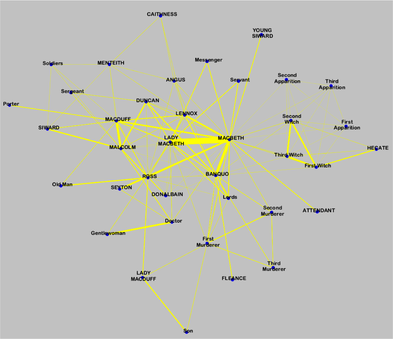
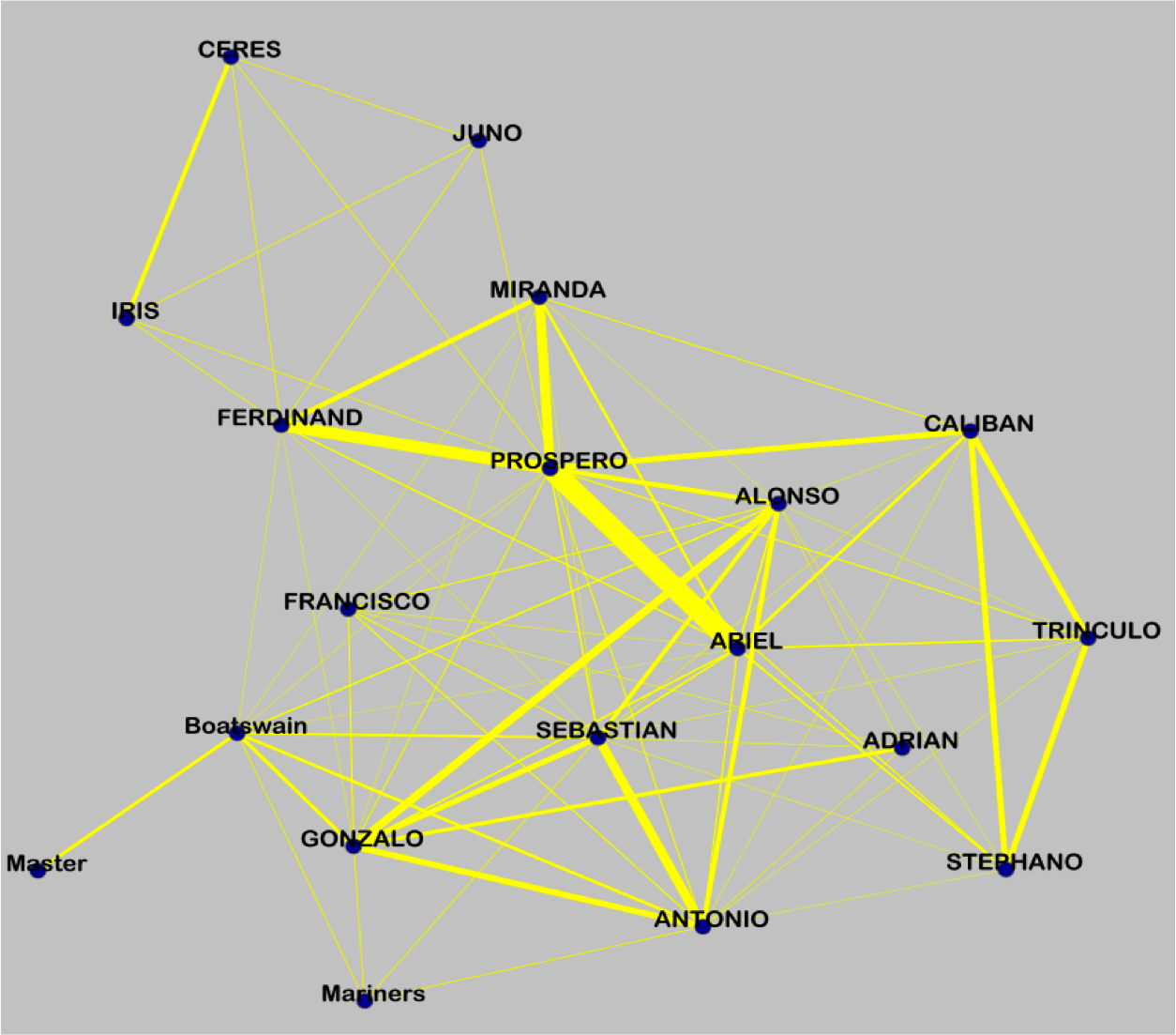
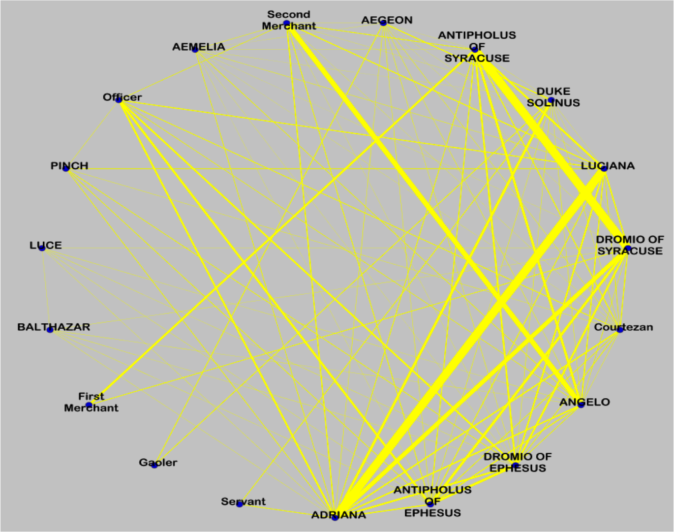
Macbeth	Tempest	A Comedy of Errors

Figure 2: Inferred weighted social networks between characters in Shakespearean plays. The thicker an edge, the stronger the tie. Tie Strength was calculated using the tie-strength measure Linear.

6 Experiments

This section presents our findings on five data sets: Shakespearean plays (Macbeth, Tempest, and A Comedy of Errors), Reality Mining, and Enron Emails.

6.1 Data Sets

Shakespearean Plays

We take three well-known plays by Shakespeare (Macbeth, Tempest, and A Comedy of Errors) and create bipartite person$\times$event graphs. The person-nodes are the characters in the play. Each event is a set of characters who are on the stage at the same time. We calculate the strength of ties between each pair of nodes. Thus without using any semantic information and even without analyzing any dialogue, we estimate how much characters interact with one another.

The Reality Mining Project

This is the popular dataset from the Reality Mining project at MIT (Eagle, Pentland, and Lazer, 2009). This study gave one hundred smart phones to participants and logged information generated by these smart phones for several months. We use the bluetooth proximity data generated as part of this project. The bluetooth radio was switched on every five minutes and logged other bluetooth devices in close proximity. The people are the participants in the study and events record the proximity between people. This gives us a total of 326,248 events.

Enron Emails

This dataset consists of emails from 150 users from the Enron corporation, that were made public during the Federal Energy Regulatory Commission investigation. We look at all emails that occur between Enron addresses. Each email is an event and all the people copied on that email i.e. the sender (from), the receivers (to, cc and bcc) are included in that event. This gives a total of 32,471 people and 371,321 events.

6.2 Measuring Coverage of the Axioms

In Section 4, we discussed axioms governing tie-strength and characterized the axioms in terms of a partial order in Theorem 11. We shall now look at an experiment to determine the “coverage” of the axioms, in terms of the number of pairs of ties that are actually ordered by the partial order.

For different datasets, we use Theorem 11 to generate a partial order between all ties. Table 2 shows the percentage of all ties that are not resolved by the partial order – i.e., the partial order cannot tells us if one tie is greater or if they are equal. Each measure of tie-strength gives a total order on the ties; and, hence resolves all the comparisons between pairs of ties. The number of tie-pairs which are left incomparable in the partial order gives a notion of the how much room the axioms leave open for different tie-strength functions to differ from each other. Table 2 shows that partial order does resolve a very high percentage of the ties. Also, we see that real-world datasets (e.g., Reality Mining) have more unresolved ties than the cleaner Shakespearean plays datasets.

Dataset	Tie Pairs	Incomparable Pairs (%)
Tempest	14,535	275 (1.89)
Comedy of Errors	14,535	726 (4.99)
Macbeth	246,753	584 (0.23)
Reality Mining	13,794,378	1,764,546 (12.79)

Table 2: Number of ties not resolved by the partial order. The last column shows the percentage of tie pairs on which different tie-strength functions can differ.

Next, we look at two tie-strength functions (Jaccard Index and Temporal Proportional) which do not obey the axioms. As previously shown, Theorem 11 implies that these functions do not obey the partial order. So, there are some tie-pairs in conflict with the partial order. Table 3 shows the number of tie-pairs that are actually in conflict. This experiment gives us some intuition about how far away a measure is from the axioms. We see that for these datasets, Temporal Proportional agrees with the partial order more than the Jaccard Index. We can also see that as the size of the dataset increases, the percentage of conflicts decreases drastically.

Dataset	Tie Pairs	Jaccard (%)	Temporal(%)
Tempest	14,535	488 (3.35)	261 (1.79)
Comedy	14,535	1,114 (7.76)	381 (2.62)
Macbeth	246,753	2,638 (1.06)	978 (0.39)
Reality	13,794,378	290,934 (0.02)	112,546 (0.01)

Table 3: Number of conflicts between the partial order and the tie-strength functions: Jaccard Index and Temporal Proportional. The second and third columns show the percentage of tie-pairs in conflict with the partial order.

6.3 Visualizing Networks

We obtain the tie strength between characters from Shakespearean plays using the linear function proposed by Linear. Figure 2 shows the inferred weighted social networks. Note that the inference is only based on people occupying the same stage and not on any semantic analysis of the text. The inferred weights (i.e. tie strengths) are consistent with the stories. For example, the highest tie strengths are between Macbeth and Lady Macbeth in the play Macbeth, between Ariel and Prospero in Tempest, and between Dromio of Syracuse and Antipholus of Syracuse in A Comedy of Errors.

6.4 Measuring Correlation among Tie-Strength Functions

Figures 3 and 4 show the frequency distributions of the number of people at an event. We see that these distributions are very different for the different graphs (even among the real-world communication networks, Enron and MIT Reality Mining). This suggests that different applications might need different measures of tie strength.

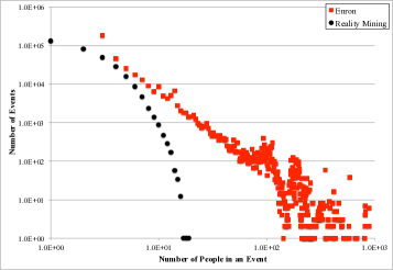
Figure 3: Frequency distribution of number of people per event for the Reality Mining and Enron datasets (in log-log scale)

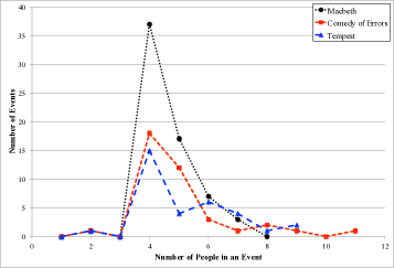
Figure 4: Frequency distribution of number of people per event for the Shakespearean Plays

Figure 4 shows Kendall’s $\tau$ coefficient for the Shakespearean plays, the Reality Mining data and Enron emails. Depending on the data set, different measures of tie strength are correlated. For instance, in the “clean” world of Shakespearean plays Common Neighbor is the least correlated measure; while in the “messy” real world data from Reality Mining and Enron emails, Max is the least correlated measure.

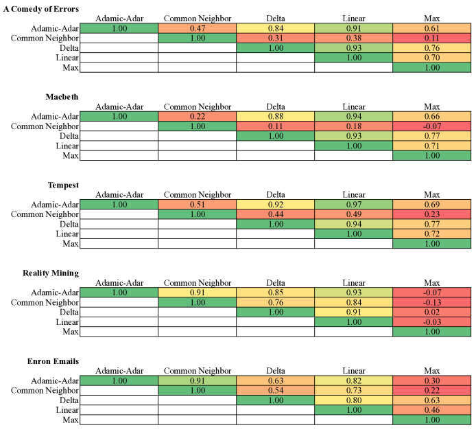
Figure 5: Kendall’s $\tau$ coefficient for Shakespearean plays, the Reality Mining data and the Enron emails. The color scale goes from bright green (coefficient = 1) to bright red (coefficient = -1). In the Skakespearean plays, the least correlated measure is Common Neighbor (as indicated by the red cells in that column). In the real-world communication networks of Enron and Reality Mining, the least correlated measure is Max (again as indicated by the red cells in that column). Since the correlation matrices are symmetric, we show only the upper-triangle entries.

7 Conclusions

We presented an axiomatic approach to the problem of inferring implicit social networks by measuring tie strength from bipartite person$\times$event graphs. We characterized functions that satisfy all axioms and demonstrated a range of measures that satisfy this characterization. We showed that in ranking applications, the axioms are equivalent to a natural partial order; and demonstrated that to settle on a particular measure, we must make a non-obvious decision about extending this partial order to a total order which is best left to the particular application. We classified measures found in prior literature according to the axioms that they satisfy. Finally, our experiments demonstrated the coverage of the axioms and revealed through the use of Kendall’s Tau correlation whether a dataset is well-behaved, where we do not have to worry about which tie-strength measure to choose, or we have to be careful about the exact choice of measure.

References

- Adamic and Adar [2003] L. A. Adamic and E. Adar. Friends and neighbors on the web. Social Networks, 25(3):211–230, 2003.
- Allali et al. [2011] O. Allali, C. Magnien, and M. Latapy. Link prediction in bipartite graphs using internal links and weighted projection. In Proceedings of the 3rd International Workshop on Network Science for Communication Networks, NetSciCom, 2011.
- Altman and Tennenholtz [2005] A. Altman and M. Tennenholtz. Ranking systems: the pagerank axioms. In Proceedings of the 6th ACM conference on Electronic Commerce, EC, pages 1–8, 2005.
- Eagle et al. [2009] N. Eagle, A. Pentland, and D. Lazer. Inferring social network structure using mobile phone data. Proceedings of the National Academy of Sciences, 106(36):15274–15278, 2009.
- Gilbert and Karahalios [2009] E. Gilbert and K. Karahalios. Predicting tie strength with social media. In Proceedings of the 27th international conference on Human factors in computing systems, CHI, pages 211–220, 2009.
- Granovetter [1973] M. Granovetter. The strength of weak ties. American Journal of Sociology, 78(6):1360–1380, 1973.
- Jeh and Widom [2002] G. Jeh and J. Widom. Simrank: A measure of structural-context similarity. In Proceedings of the International Conference on Knowledge Discovery and Data Mining, KDD, pages 538–543, 2002.
- Kahanda and Neville [2009] I. Kahanda and J. Neville. Using transactional information to predict link strength in online social networks. In Proceedings of the 3rd Conference on Weblogs and Social Media, ICWSM, 2009.
- Karzanov and Khachiyan [1991] A. Karzanov and L. Khachiyan. On the conductance of order markov chains. Order, 8(1):7–15, 1991.
- Katz [1953] L. Katz. A new status index derived from sociometric analysis. Psychometrika, 18(1):39–43, 1953.
- Liben-Nowell and Kleinberg [2003] D. Liben-Nowell and J. Kleinberg. The link prediction problem for social networks. In Proceedings of the 12th International Conference on Information and Knowledge Management, CIKM, pages 556–559, 2003.
- Lin [1998] D. Lin. An information-theoretic definition of similarity. In Proceedings of the Fifteenth International Conference on Machine Learning, ICML, pages 296–304, 1998.
- Roth et al. [2010] M. Roth, A. Ben-David, D. Deutscher, G. Flysher, I. Horn, A. Leichtberg, N. Leiser, Y. Matias, and R. Merom. Suggesting friends using the implicit social graph. In Proceedings of the 16th Conference on Knowledge Discovery and Data Mining, KDD ’10, pages 233–242, 2010.