Nonlinear stability of phase-locked states for the Kuramoto model with finite inertia

Abstract

We discuss the nonlinear stability of phase-locked states for globally coupled nonlinear oscillators with finite inertia, namely the modified Kuramoto model, in the context of the robust $\ell^{\infty}$-norm. We show that some classes of phase-locked states are orbitally $\ell^{\infty}$-stable in the sense that its small perturbation asymptotically leads to only the phase shift of the phase-locked state from the original one without changing its fine structures as keeping the same suitable coupling strength among oscillators and the same natural frequencies. The phase shift is uniquely determined by the average of initial phases, the average of initial frequencies, and the strength of inertia. We numerically confirm the stability of the phase-locked state as well as its uniqueness and the phase shift, where various initial conditions are considered. Finally, we argue that some restricted conditions employed in the mathematical proof are not necessary, based on numerical simulation results.

1 Introduction

Since Kuramoto introduced a mathematical model of coupled nonlinear oscillators Ku by refining the earlier Winfree’s model Wi to be more mathematically tractable, it has become a minimal model for collective synchronization phenomena, which are ubiquitous in real systems ranging from physics to biology. The original Kuramoto model is very simple but exhibits lots of rich behaviors including a synchronization transition, where all the oscillators’ phases are tuned by the coupling strength against the diversity of natural frequencies, and eventually reach a phase-locked state (frequency entrainment) including in-phase synchronization with exactly the same value (see A-B ; Da for detailed discussion).

Synchronization is a quite interesting nonlinear phenomenon, which can yield a dynamic phase transition against the coupling strength among weakly coupled oscillators for a given natural frequency distribution. Above the coupling strength threshold, oscillators become partially phase-locked, which is called partial synchronization. The existence of partially phase-locked solutions and their stability were studied by Kuramoto Ku and Crawford Cr , respectively. As an extension of the aforementioned works, Aeyels and Rogge addressed the stability issue for networks of a finite number of oscillators A-R , and Mirollo and Strogatz analyzed the linear stability of phase-locked states for globally coupled Kuramoto oscillators M-S . Later on, lots of phase models have been proposed to describe the dynamic behavior of large populations of nonlinearly coupled oscillators. Furthermore, it has also been widely discussed that the nature of synchronization transitions for the continuum version of the original Kuramoto model is subject to the shape of the natural frequency distribution function. While the synchronization transition has been widely discussed from the physical point of view, the strict shape of phase-locked states has not drawn much less attention because it concerns far from the transition. Of course, the transition is one of the interesting topics to be studied in many senses, such as critical behaviors and its universality issue. However, it is mostly restricted to numerical studies, which implies that there are always some technical difficulties to reach a correct conclusion without rigorous mathematical guidelines and/or proofs. In that sense, it is meaningful if we can report what and how can be mathematically proven in the perspective of relevant aspects directly and indirectly to major interests for a given model before proceeding numerical studies near and at the transition.

In this paper, we address the modified Kuramoto model with finite inertia and take an interest with the details of phase-locked states in order to handle the shape of phase-locked states as well as their uniqueness issue for a fixed distribution of natural frequencies. Consider an ensemble of finite number of Kuramoto oscillators with finite inertia. Let $\theta_{i}=\theta_{i}(t)$ be the phase of the $i$-th oscillator and $m$ denotes the strength of uniform inertia acting on Kuramoto oscillators. In this situation, the dynamics of $\theta_{i}$ is governed by the initial valule problem of second-order ODEs:

$$m{\ddot{\theta}}_{i}+{\dot{\theta}}_{i}=\Omega_{i}+\frac{K}{N}\sum_{j=1}^{N}\sin(\theta_{j}-\theta_{i}),\quad t>0,\quad i=1,...,N,$$ (1.1)

subject to initial phase-frequency configuration:

$$(\theta_{i},{\dot{\theta}}_{i})(0)=(\theta_{i0},\omega_{i0}=\dot{\theta}_{i0}).$$ (1.2)

Without loss of generality, we assume that the average of natural frequencies is zero:

$$\Omega_{c}:=\frac{1}{N}\sum_{i=1}^{N}\Omega_{i}\equiv 0.$$ (1.3)

The system (1.1) was first introduced by Ermentrout Er as a phenomenological model to explain the slow synchronization of certain biological systems, e.g., fireflies of the Pteroptyx malaccae, and this model has been used to describe various dynamical systems A-S2 ; D-D-T ; P-C ; W-C-S1 ; W-C-S2 ; W-S0 ; W-St ; W-S . The whole review and mathematical results for the Kuramoto model can be found in A-B ; S-M1 ; S-M2 ; S-S-W . In the earlier study, the first author and his collaborators C-H-Y have verified that for some classes of initial configurations and $mK\geq\frac{1}{4}$, the speed to the phase-locked states is slower than that of the original Kuramoto model (without the inertial term), which illustrates the slow relaxation of Kuramoto oscillators.

The main novelty of this paper is to provide a simple proof for the nonlinear stability of some classes of phase-locked states in globally coupled Kuramoto oscillators with finite inertia. Using the robust $\ell^{\infty}$-norm, we present the proof under the suitable conditions on initial phase-frequency configurations, coupling strengths, and finite inertia. It is noted that phase-locked states are orbitally $\ell^{\infty}$-stable, which results in the uniqueness of phase-locked states.

This paper is organized after introduction as follows. In Sec. 2, we briefly recall some basic definitions and mathematical structures od the system (1.1). In Sec. 3, we show the proof of orbital stability of phase-locked states and provide extensive numerical simulations, which confirm our analytical results. Finally, Section 4 is devoted to the summary of main results and the conclusion of the paper.

2 Frameworks and main results

In this section, we discuss two frameworks depending on the relative size of inertial strength and present main results on the orbital stability of phase-locked states. We also present several mathematical structures of the system (1.1)-(1.3), and recall a second-order Gronwall’s lemma from C-H-Y which will be used in the proof of our main result.

Before we begin our technical discussions, we first recall several definitions for the phase-locked state and its orbital stability as follows.

Definition 2.1

(Phase-locked state and orbital stability)

1. Let $\theta(t):=(\theta_{1}(t),\cdots,\theta_{N}(t))\in\mathbb{T}^{N}$ be the solution to the system (1.1) - (1.3). Then $\theta$ is (strongly) phase-locked if and only if $\theta$ is an equilibrium solution to the system of ODEs (1.1), i.e.,

   $$\Omega_{i}+\frac{K}{N}\sum_{i=1}^{N}\sin(\theta_{j}-\theta_{i})=0,\qquad{\dot{\theta}}_{i}=0.$$

2. Let $\theta$ and ${\tilde{\theta}}$ be two phase-locked solutions to the system (1.1) and (1.3). Then, $\theta$ and ${\tilde{\theta}}$ are congruent and denoted if and only if there exists a constant $\beta\in R$ such that

   $$\theta-{\tilde{\theta}}=\beta{\mathbb{I}}_{N},$$

   where ${\mathbb{I}}_{N}:=(1,\cdots,1)\in\mathbb{Z}^{N}$.

3. Let $\theta^{e}$ be a phase-locked solution to the system (1.1) and (1.3). Then $\theta^{e}$ is orbitally stable if and only if for any initial phase-configuration $\theta_{0}$ close to $\theta^{e}$ in a norm $||\cdot||$, the solution $\theta(t)$ converges to the phase-shift of $\theta^{e}$ in a norm $||~{}\cdot~{}||$ as $t\to\infty$, i.e.,

   $$\lim_{t\to\infty}||\theta(t)-(\theta^{e}+\beta\mathbb{I}_{N})||=0,\quad\mbox{for some constant $\beta$}.$$

Below we add some comments on the above definitions.

Remark 2.1

1. In general, a phase-locked state is a traveling profile with a constant phase velocity $\Omega_{c}$.

2. The time-dependent solution $\theta=\theta(t)$ is a (weakly) phase-locked state if and only if there exist positive constants $C_{*},C^{*}\geq 0$ independent of $t$ satisfying

   $$C_{*}\leq|\theta_{i}(t)-\theta_{j}(t)|\leq C^{*},\quad t\geq 0.$$

2.1 Basic estimates

We rewrite the system (1.1) as a system of first-order ODEs for $(\theta_{i},\omega_{i}:={\dot{\theta}}_{i})$:

$$\begin{aligned} \displaystyle{\dot{\theta}}_{i}&=\omega_{i},\quad t>0,~{}~{}i=1,\cdots,N,\\ \displaystyle{\dot{\omega}}_{i}&=\frac{1}{m}\Big{(}-\omega_{i}+\Omega_{i}+\frac{K}{N}\sum_{j=1}^{N}\sin(\theta_{j}-\theta_{i})\Big{)}.\end{aligned}$$ (2.1)

We next introduce macro variables (center-of-mass frame) and micro variables (fluctuations around macro variables):

$$\theta_{c}:=\frac{1}{N}\sum_{i=1}^{N}\theta_{i},\quad\omega_{c}:=\frac{1}{N}\sum_{i=1}^{N}\omega_{i},\quad{\hat{\theta}}_{i}:=\theta_{i}-\theta_{c},\quad{\hat{\omega}}_{i}:=\omega_{i}-\omega_{c},$$

Then, macro-variables and micro-variables satisfy, respectively,

$${\dot{\theta}}_{c}=\omega_{c},\quad{\dot{\omega}}_{c}=-\frac{\omega_{c}}{m},$$ (2.2)

and

$$\begin{aligned} {\dot{\hat{\theta}}}_{i}&={\hat{\omega}}_{i},\quad m{\dot{\hat{\omega}}}_{i}&=-{\hat{\omega}}_{i}+{\hat{\Omega}}_{i}+\frac{K}{N}\sum_{j=1}^{N}\sin({\hat{\theta}}_{j}-{\hat{\theta}}_{i}).\end{aligned}$$ (2.3)

By direct calculations,

$$\theta_{c}(t)=\theta_{c}(0)+m\omega_{c}(0)(1-e^{-\frac{t}{m}}),\quad\omega_{c}(t)=e^{-\frac{t}{m}}\omega_{c}(0).$$

Thus, macro-variables converge toward some constant states that are determined by their initial configurations and the magnitude of inertia:

$$\lim_{t\to\infty}(\theta_{c}(t),\omega_{c}(t))=(\theta_{c}(0)+m\omega_{c}(0),0).$$ (2.4)

For convenience, we recall the following second-order differential inequality:

$$\begin{aligned} &a{\ddot{y}}+b{\dot{y}}+cy+d\leq 0,\quad t>0,\\ &y(0)=y_{0},\quad{\dot{y}}(0)=y_{1},\end{aligned}$$ (2.5)

where $a>0,b,c$ and $d$ are constants.

Lemma 2.1

C-H-Y Let $y=y(t)$ be a nonnegative $C^{2}$-function satisfying the differential inequality (LABEL:DI-1). Then we have following relations:

$$(i)~{}b^{2}-4ac>0;$$

$$y(t)\leq\Big{(}y_{0}+\frac{d}{c}\Big{)}e^{-\nu_{1}t}+a\frac{e^{-\nu_{2}t}-e^{-\nu_{1}t}}{\sqrt{b^{2}-4ac}}\Big{(}y_{1}+\nu_{1}y_{0}+\frac{2d}{b-\sqrt{b^{2}-4ac}}\Big{)}-\frac{d}{c}.$$

$$(ii)~{}b^{2}-4ac\leq 0;$$

$$y(t)\leq e^{-\frac{b}{2a}t}\Big{[}y_{0}+\frac{4ad}{b^{2}}+\Big{(}\frac{b}{2a}y_{0}+y_{1}+\frac{2d}{b}\Big{)}t\Big{]}-\frac{4ad}{b^{2}},$$

where decay exponents $\nu_{1}$ and $\nu_{2}$ are given as follows.

$$\nu_{1}:=\frac{b+\sqrt{b^{2}-4ac}}{2a},\quad\nu_{2}:=\frac{b-\sqrt{b^{2}-4ac}}{2a}.$$

2.2 Main results

In order to present main results regarding the stability of phase-locked states, we first discuss two frameworks, which depend on the relative magnitude of inertia $m$ to the strength of coupling $K$ between oscillators.

Let us recall a $\ell^{p}$-norm for a finite-dimensional vector space. For $\theta\in\mathbb{T}^{N}$, the $\ell^{p}$-norm of $\theta$ is defined as follows.

$$||\theta||_{\ell^{p}}:=\left\{\begin{array}[]{ll}\displaystyle\Big{(}\sum_{i=1}^{N}|\theta_{i}|^{p}\Big{)}^{\frac{1}{p}},&p\in[1,\infty),\\ \displaystyle\max_{1\leq i\leq N}|\theta_{i}|,&p=\infty.\end{array}\right.$$

Then, phase and natural frequency diameters can be denoted as

$$D(\theta):=\max_{1\leq i,j\leq N}|\theta_{i}-\theta_{j}|\quad\mbox{and}\quad D(\Omega):=\max_{1\leq i,j\leq N}|\Omega_{i}-\Omega_{j}|.$$

It is noted that for $\theta\in\mathbb{T}^{N}$ with $\sum_{i=1}^{N}\theta_{i}=0$, $||\theta||_{\ell^{\infty}}$ and $D(\theta)$ are equivalent in the sense that

$$||\theta||_{\ell^{\infty}}\leq D(\theta)\leq 2||\theta||_{\ell^{\infty}}.$$

The following two frameworks that concern the magnitude of inertia were first introduced in C-H-Y for the existence of phase-locked states to the system (1.1).

$\bullet$ Framework A: (Small inertia regime)

1. The strength of coupling $K$ and the magnitude of inertia $m$ satisfy

   $$0<D(\Omega)<K,\qquad mK<\frac{D^{\infty}}{4\sin D^{\infty}},$$

   where $D^{\infty}\in\Big{(}0,\frac{\pi}{2}\Big{)}$ is the root of the following trigonometric equation:

   $$\sin x=\frac{D(\Omega)}{K}.$$

2. An initial configuration of $(\theta_{0},\omega_{0})$ satisfies

   $$0<\max\Big{\{}D(\theta_{0}),D(\theta_{0})+2m{\dot{D}}(\theta(t))\Big{|}_{t=0}\Big{\}}<D^{\infty},$$

$\bullet$ Framework B: (Large inertia regime)

1. The strength of coupling $K$ and the magnitude of inertia $m$ satisfy

   $$0<D(\Omega)<\frac{\pi}{8m},\qquad mK>\frac{\pi}{8}.$$

2. An initial configuration of $(\theta_{0},\omega_{0})$ satisfies

   $$0<\max\Big{\{}D(\theta_{0}),D(\theta_{0})+2m{\dot{D}}(\theta(t))\Big{|}_{t=0}\Big{\}}<4mD(\Omega).$$

We also note that for $D^{\infty}\in\Big{(}0,~{}\frac{\pi}{2}\Big{)}$,

$$\frac{D^{\infty}}{4\sin D^{\infty}}<\frac{\pi}{8}.$$

By definitions, Framework A and Framework B correspond some restricted cases of $mK$. Let ${\mathcal{P}}$ be the collection of all phase-locked states evolved from various initial configurations satisfying either Framework A or Framework B, i.e.,

$${\mathcal{P}} := \{\theta^{e}=(\theta^{e}_{1},\cdots,\theta^{e}_{N})\in\mathbb{T}^{N}~{}:~{}\theta^{e}:=\lim_{t\to\infty}\theta(t),\quad\mbox{where $\theta(t)$ is the solution to the system \eqref{main} -\eqref{nat} }$$

$$\hskip 56.9055pt\mbox{ with initial datum $\theta_{0}$ satisfying either Framework A or Framework B }\}.$$

The set ${\mathcal{P}}$ is a proper subset of all possible phase-locked states for the system (1.1) and (1.3) (see Section 3.2), and phase-locked states in ${\mathcal{P}}$ have a diameter strictly less than $\frac{\pi}{2}$.

We now move onto the main results of this paper, the orbital stability of phase-locked states.

Theorem 2.1

(Orbital stability)
Suppose either Framework A or Framework B hold, and let $\theta^{e}$ be a given phase-locked state in ${\mathcal{P}}$. Then $\theta^{e}$ is orbitally $\ell^{\infty}$-stable in the sense that for any perturbed initial configuration ${\tilde{\theta}}_{0}$ satisfying the condition (2) in either Framework A or Framework B, the perturbed solution ${\tilde{\theta}}(t)$ satisfies

$$\lim_{t\to\infty}||{\tilde{\theta}}(t)-(\theta^{e}+(\Delta\theta)^{\infty}\mathbb{I}_{N})||_{\ell^{\infty}}=0,$$

where the phase-shift $(\Delta\theta)^{\infty}$ is explicitly given by

$$(\Delta\theta)^{\infty}:=\theta^{e}_{c}-{\tilde{\theta}}_{c}(0)-m{\tilde{\omega}}_{c}(0).$$

Remark 2.2

1. The conditions of Framework A and Framework B are independent of the system size $N$. Hence, our results can be lifted to the kinetic regime via the thermodynamic limit.

2. Under both Framework A and Framework B, the initial phase-frequency configuration $(\theta_{0},\omega_{0})$ evolves toward the asymptotic phase-locked state $(\theta^{\infty},0)$:

$$\Omega_{i}+\frac{K}{N}\sum_{i=1}^{N}\sin(\theta^{\infty}_{j}-\theta^{\infty}_{i})=0,\qquad\sup_{t\geq 0}D(\theta(t))<\frac{\pi}{2}.$$

3. For the case of $m=0$ (the original Kuramoto model), the orbital stability of phase-locked states is provided in C-H-J-K using the $\ell^{1}$-contraction theory:

$$\lim_{t\to\infty}||\tilde{\theta}(t)-(\theta^{e}+(\Delta\theta)^{\infty}\mathbb{I}_{N})||_{\ell^{1}}=0.$$

However, we cannot apply this estimate to the system (1.1) due to inertia. Thus, we employ a new estimate to include the previous result and also cover the inertial effect, which is based on $\ell^{\infty}$-metric.

4. Theorem 2.1 implies that a phase-locked state with the phase diameter $D(\theta)$ strictly less than $\frac{\pi}{2}$ is unique up to the phase shift. Let $\theta$ and $\tilde{\theta}$ be the two phase-locked states emerged from initial data $(\theta_{0},\omega_{0})$ and $(\tilde{\theta}_{0},\tilde{\omega}_{0})$, respectively. Suppose that

$$D(\theta^{\infty}),~{}D(\tilde{\theta}^{\infty})<\frac{\pi}{2}.$$

Then, by the same argument as in Theorem 2.1, we have

$$\theta^{\infty}-\tilde{\theta}^{\infty}=\Big{(}\theta_{c}(0)-\tilde{\theta}_{c}(0)+m(\omega_{c}(0)-\tilde{\omega}_{c}(0))\Big{)}\mathbb{I}_{N}.$$

3 Nonlinear stability of phase-locked states

In this section, we claim the orbital nonlinear stability of the phase-locked states in the $\ell^{\infty}$ norm as providing some analytical proof, which is also numerically confirmed.

3.1 The proof of Theorem 2.1

Suppose either Framework A or Framework B hold, and let $\theta^{e}$ be a given phase-locked state in ${\mathcal{P}}$ with $D(\theta^{e})<\frac{\pi}{2}$ and ${\tilde{\theta}}_{0}$ be a perturbed phase-configuration of $\theta^{e}$. Then, thanks to Theorem 2.1, the perturbed configuration ${\tilde{\theta}}={\tilde{\theta}}(t)$ with the initial configuration ${\tilde{\theta}}_{0}$ satisfies

$$D(\theta^{e})+D({\tilde{\theta}}(t))<\pi,\qquad t\geq 0.$$

We set

$$\alpha_{i} := \theta^{e}_{i}-{\tilde{\theta}}_{i},\quad\alpha_{c}(t):=\frac{1}{N}\sum_{i=1}^{N}\alpha_{i}(t),\quad\hat{\alpha}_{i}(t):=\alpha_{i}(t)-\alpha_{c}(t),$$

$$\hat{\alpha}_{M} := \max_{1\leq i\leq N}\hat{\alpha}_{i},\quad\hat{\alpha}_{m}:=\min_{1\leq i\leq N}\hat{\alpha}_{i},\quad D(\alpha(t))=\hat{\alpha}_{M}-\hat{\alpha}_{m}.$$

Note that

$$\begin{aligned} \alpha_{c}(t)&=\theta^{e}_{c}-\tilde{\theta}_{c}(t)=\theta^{e}_{c}-\tilde{\theta}_{c}(0)-m(1-e^{-\frac{t}{m}})\tilde{\omega}_{c}(0),\\ &\to\theta^{e}_{c}-\tilde{\theta}_{c}(0)-m\tilde{\omega}_{c}(0),\quad\mbox{as $t\to\infty$},\\ |\alpha_{j}(t)-\alpha_{i}(t)|&=|\theta^{e}_{j}-\tilde{\theta}_{j}(t)-(\theta^{e}_{i}-\tilde{\theta}_{i}(t))|\leq D(\theta^{e})+D({\tilde{\theta}}(t))<\pi,\quad\mbox{for}\quad t\geq 0.\end{aligned}$$ (3.1)

By simple calculations, we obtain

$$m\frac{d^{2}\hat{\alpha}_{i}}{dt^{2}}+\frac{d\hat{\alpha}_{i}}{dt}=\frac{2K}{N}\sum_{j=1}^{N}\cos\Big{(}\frac{\theta^{e}_{j}-\theta^{e}_{i}}{2}+\frac{{\tilde{\theta}}_{j}-{\tilde{\theta}}_{i}}{2}\Big{)}\sin\Big{(}\frac{\hat{\alpha}_{j}-\hat{\alpha}_{i}}{2}\Big{)}.$$ (3.2)

$\bullet$ Step A (Derivation of Gronwall’s inequality for $D(\alpha)$):

It follows from (3.2) that

$$\begin{aligned} m\frac{d^{2}\hat{\alpha}_{M}}{dt^{2}}+\frac{d\hat{\alpha}_{M}}{dt}&=\frac{2K}{N}\sum_{j=1}^{N}\cos\Big{(}\frac{\theta^{e}_{j}-\theta^{e}_{i}}{2}+\frac{{\tilde{\theta}}_{j}-{\tilde{\theta}}_{i}}{2}\Big{)}\sin\Big{(}\frac{\hat{\alpha}_{j}-\hat{\alpha}_{M}}{2}\Big{)}\\ &\leq\Big{(}\frac{K\sin 2D_{0}^{av}}{D_{0}^{av}N}\Big{)}\sum_{j=1}^{N}\Big{(}\frac{\hat{\alpha}_{j}-\hat{\alpha}_{M}}{2}\Big{)}\\ &=-\frac{K\sin 2D_{0}^{av}}{2D_{0}^{av}}{\hat{a}}_{M},\end{aligned}$$ (3.3)

where we used the fact $-\pi<\hat{\alpha}_{j}-\hat{\alpha}_{M}\leq 0$ to find

$$D_{0}^{av}:=\frac{D(\theta^{e})+D({\tilde{\theta}}_{0})}{2},\quad\sum_{i=1}^{N}\hat{\alpha}_{i}=0,$$

$$\sin\Big{(}\frac{\hat{\alpha}_{j}-\hat{\alpha}_{M}}{2}\Big{)}\leq\Big{(}\frac{\sin D_{0}^{av}}{D_{0}^{av}}\Big{)}\Big{(}\frac{\hat{\alpha}_{j}-\hat{\alpha}_{M}}{2}\Big{)}.$$

Similarly, we find

$$m\frac{d^{2}\hat{\alpha}_{m}}{dt^{2}}+\frac{d\hat{\alpha}_{m}}{dt}\geq-\frac{K\sin 2D_{0}^{av}}{2D_{0}^{av}}{\hat{a}}_{m}.$$ (3.4)

We combine the estimates (3.3) and (3.4) to find

$$m\frac{d^{2}D({\alpha})}{dt^{2}}+\frac{dD(\alpha)}{dt}+\bar{K}D({\alpha})\leq 0,\qquad\bar{K}:=\frac{K\sin 2D_{0}^{av}}{2D_{0}^{av}}.$$ (3.5)

$\bullet$ Step B (Decay estimates of $D(\alpha)$):

We apply Lemma 2.1 for (3.5) to obtain

$$D(\alpha(t))\leq\left\{\begin{array}[]{ll}D({\alpha}_{0})e^{-\mu_{1}t}+m\frac{e^{-\mu_{2}t}-e^{-\mu_{1}t}}{\sqrt{1-4m\bar{K}}}\Big{(}{\dot{D}}(\alpha_{0})+\mu_{1}D({\alpha}_{0})\Big{)},&1-4m\bar{K}>0,\\ e^{-\frac{t}{2m}}\Big{[}D({\alpha}_{0})+\Big{(}\frac{1}{2m}D({\alpha}_{0})+\dot{D}({\alpha}_{0})\Big{)}t\Big{]},&1-4m\bar{K}\leq 0,\end{array}\right.$$

where

$$\mu_{1}=\frac{1+\sqrt{1-4m\bar{K}}}{2m},\quad\mu_{2}=\frac{1-\sqrt{1-4m\bar{K}}}{2m}.$$

Hence, for any $\varepsilon\in\Big{(}0,\frac{1}{2m}\Big{)}$, we have

$$D({\alpha}(t))\approx{\mathcal{O}}(1)e^{-\lambda(\varepsilon)t}\quad\mbox{for~{}large~{}time}t,\quad\lambda(\varepsilon):=\min\Big{\{}\mu_{2},\frac{1}{2m}-\varepsilon\Big{\}}.$$

We set

$$(\Delta\theta)^{\infty}:=\theta^{e}_{c}-{\tilde{\theta}}_{c}(0)-m{\tilde{\omega}}_{c}(0).$$

Using the triangle inequality, we get the following results:

$$||\theta^{e}-{\tilde{\theta}}(t)-(\Delta\theta)^{\infty}\mathbb{I}_{N}||_{\ell^{\infty}} = ||\alpha(t)-(\Delta\theta)^{\infty}\mathbb{I}_{N}||_{\ell^{\infty}}$$

$$\leq ||\alpha(t)-\alpha_{c}(t)|+|\alpha_{c}(t)-(\Delta\theta)^{\infty}\mathbb{I}_{N}||_{\ell^{\infty}}$$

$$\leq 2D(\alpha(t))+||\alpha_{c}(t)-(\Delta\theta)^{\infty}\mathbb{I}_{N}||_{\ell^{\infty}},$$

which implies

$$\lim_{t\to\infty}||{\tilde{\theta}}(t)-(\theta^{e}+(\Delta\theta)^{\infty}\mathbb{I}_{N})||_{\ell^{\infty}}=0.$$

This completes the proof.

3.2 Numerical simulations

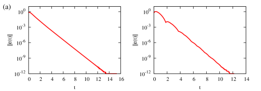
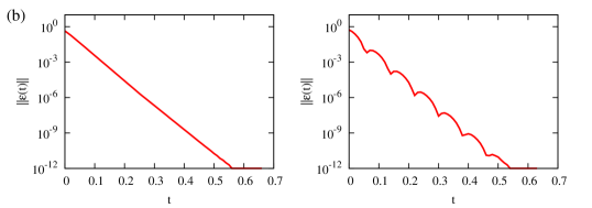
Figure 1: (Color online) Semi-logarithmic plots of the relative error, $||{\mathcal{E}}(t)||$, against time, $t$, which show the exponential decay for various conditions: $N=100$ and 100 realizations from $\{\theta_{i}(0)\}\subset[-\frac{\pi}{10},\frac{\pi}{10}]$, and $\{\omega_{i}(0)\}\subset[-\pi,\pi]$. We test two different distributions of natural frequencies, (a) for the uniform distribution, Framework A (left) with ($m$=0.1, $K$=2.0) and Framework B (right) with ($m$=0.2, $K$=2.0) and (b) for Cauchy (Lorentzian) distribution, Framework A (left) with ($m$=0.004, $K$=40.0) and Framework B (right) with ($m$=0.01, $K$=40.0).

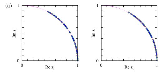
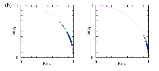
Figure 2: (Color online) Three different phase-locked states ($\circ,~{}\times,~{}+$) on complex plane, which coincide with one another by the rotation with the relative phase-shift for $N=100$, $\{\theta_{i}(0)\}\subset[-\frac{\pi}{10},\frac{\pi}{10}]$, and $\{\omega_{i}(0)\}\subset[-\pi,\pi]$. Two different distributions of natural frequencies are tested with the same setups of Fig. 1, summarized in Table 1. The dashed line on the complex plane is guided for eyes as drawing an unit circle whose center is located at the origin point.

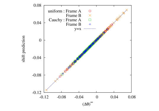
Figure 3: (Color online) For phase-locked states, the analytic estimate (Theorem 2.1) of the relative phase-shift is confirmed in Framework A and Framework B with two distributions of natural frequencies: the uniform distribution and the Cauchy distribution, respectively. We plot all the cases of Figs. 1 and  2, summarized in Table 1. Our numerical simulations and analytical estimates are in perfect agreement with the guide line of $y=x$.

Table 1: All the conditions and parameter sets used in our simulation tests for random 100 realizations of $\theta(0)\in[-\pi/10,\pi/10]$ and $\omega(0)\in[-\pi,\pi]$:

	$\Omega$ Distribution	Framework	m	K
Fig1,2(a)left	uniform($[-1,1]$)	A	0.1	2.0
Fig1,2(a)right	uniform($[-1,1]$)	B	0.2	2.0
Fig1,2(b)left	Cauchy($\gamma=1$)	A	0.004	40.0
Fig1,2(b)right	Cauchy($\gamma=1$)	B	0.01	40.0
Fig4,5(a)left	uniform($[-1,1]$)	-	1.0	3.0
Fig4,5(a)right	uniform($[-1,1]$)	-	0.2	2.0
Fig4,5(b)left	Cauchy($\gamma=1$)	-	0.5	40.0
Fig4,5(b)right	Cauchy($\gamma=1$)	-	0.1	20.0

Table 2: The values in the center of mass frame for selected three initial conditions among 100 realizations for Figs. 2 and  5.

Sample No.	$\theta_{c}(0)$	$\omega_{c}(0)$
1	0.020411279668	-0.056797709228
2	0.015377250725	0.283280670045
3	0.022909592396	-0.004959481400

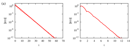
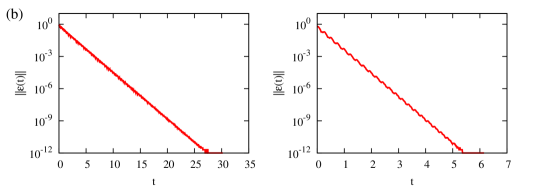
Figure 4: (Color online) Semi-logarithmic plots of the relative error, $||{\mathcal{E}}(t)||$, against time, $t$, which show the exponential decay for various conditions: $N=100$ and 100 realizations from $\{\theta_{i}(0)\}\subset[-\frac{\pi}{10},\frac{\pi}{10}]$, and $\{\omega_{i}(0)\}\subset[-\pi,\pi]$. We test two different distributions of natural frequencies, (a) for the uniform distribution, ($m$=1.0, $K$=3.0) (left) and ($m$=0.2, $K$=2.0) (right), and (b) for the Cauchy distribution, ($m$=0.5, $K$=40.0) (left) and ($m$=0.1, $K$=20.0) (right). Note that these parameter setups satisfy neither Framework A nor Framework B.

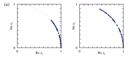
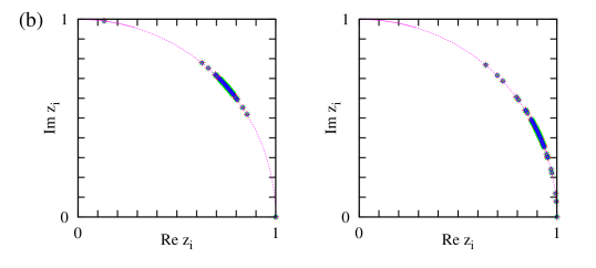
Figure 5: (Color online) Three different phase-locked states ($\circ,~{}\times,~{}+$) on complex plane, which coincide with one another by the rotation with the relative phase-shift for $N=100$, $\{\theta_{i}(0)\}\subset[-\frac{\pi}{10},\frac{\pi}{10}]$, and $\{\omega_{i}(0)\}\subset[-\pi,\pi]$. Two different distributions of natural frequencies are tested with the same setups of Fig. 4, summarized in Table 1. The dashed line on the complex plane is guided for eyes as drawing an unit circle whose center is located at the origin point.

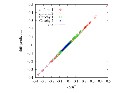
Figure 6: (Color online) For phase-locked states, the analytic estimate (Theorem 2.1) of the relative phase-shift is confirmed in Framework A and Framework B with two distributions of natural frequencies: the uniform distribution and the Cauchy distribution, respectively. We plot all the cases of Figs. 4 and  5, summarized in Table 1. Our numerical simulations and analytical estimates are in perfect agreement with the guide line of $y=x$.

In order to confirm our analytic proof and its validity, we numerically test various situations, which is delineated as follows. We employ the 4th order Runge-Kutta method to numerically integrate the modified Kuramoto model, Eq. (1.1), where

$$\mbox{the time step}~{}~{}\Delta t=10^{-2}\quad\mbox{and}\quad N=100.$$

As the natural frequency distribution, we consider

$$g_{c}(\Omega)=\frac{1}{\pi(\Omega^{2}+1)}~{}:~{}\mbox{Cauchy distribution},\qquad g_{u}(\Omega)=\frac{1}{2}{\bf 1}_{[-1,1]}~{}:~{}\mbox{uniform distribution}.$$

One Half of natural frequencies are randomly chosen from the given analytic distribution form in the positive part $\Omega>0$, and the other half is set to be negative of chosen values, so that the mean of $\Omega_{i}$ set to be 0. Initial configurations of $\{\{\theta_{i}(0)\},\{\omega_{i}(0)=\dot{\theta}_{i}(0)\}\}$ are uniformly chosen from the intervals: $\theta_{i}\in\Big{[}-\frac{\pi}{10},\frac{\pi}{10}\Big{]}$ and $\omega_{i}\in[-\pi,\pi]$ at time $t=0$, respectively.

The following procedure is how we obtain numerical results in this paper: Prepare several sets of natural frequencies and initial conditions, $\{\{\Omega_{i}\},\{\theta_{i}(0)\},\{\omega_{i}(0)\}\}$. Among them, pick up a set, $\{\{\Omega^{\rm locked}_{i}\},\{\theta^{(0)}_{i}(0)\},\{\omega^{(0)}_{i}(0)\}\}$ with which oscillators converge to a phase-locked state. In this paper, we test various initial setups, including the simplest ones: the case for initially static, $\omega_{i}(0)=0$ for any oscillators, and the case for Kuramoto-type dynamic, $\omega_{i}(0)=\Omega_{i}+\frac{K}{N}\sum_{j=1}^{N}{\sin(\theta_{j}-\theta_{i})}$. We find that for random initial configurations, there are no significant difference between numerical results in the steady state. As a result, we can detect phase-locked states as checking the condition $|\theta_{i}(t+dt)-\theta_{i}(t)|<\varepsilon$ at every time step, where we set $\varepsilon=10^{-13}$. If all phases satisfy the given condition, we assume that the system reaches the neighborhood of phase-locked states.

In Fig. 1, we first check out the 4th statement in Remark 2.2 with Framework A and Framework B as stated in Sec. 3, where without loss of generality, we take $\theta(0)\in\Big{[}-\frac{\pi}{10},\frac{\pi}{10}\Big{]}$ and $\omega(0)\in[-\pi,\pi]$ and measure the relative error from one phase-locked state to one another as follows:

$${\mathcal{E}}(t):={\mathcal{E}}(t)-{\mathcal{E}}_{c}(0),\quad{\mathcal{E}}(t):=\theta(t)-\tilde{\theta}(t),\quad{\mathcal{E}}_{c}(0):=\Big{(}\theta_{c}(0)-\tilde{\theta}_{c}(0)+m(\omega_{c}(0)-\tilde{\omega}_{c}(0))\Big{)}\mathbb{I}_{N},$$

where $\tilde{X}$ and $X_{c}$ correspond to the perturbed value from one selected setting and the value in the “center of mass” frame, respectively. The values used in our calculation are shown in Table 2. As expected, the relative error $||{\mathcal{E}}(t)||$ decays exponentially fast to zero, which is the numerical verification of Theorem 2.1 as well.

Once $\{\Omega_{i}\}=\{\Omega^{\rm locked}_{i}\}$ is found, we then fix it as the natural frequency distribution and change the initial conditions of $\{\{\theta_{i}(0)\},\{\omega_{i}(0)\}\}$. With the set $\{\{\Omega^{\rm locked}_{i}\},\{\theta^{(1)}_{i}(0)\},\{\omega^{(1)}_{i}(0)\}\}$, $\{\{\Omega^{\rm locked}_{i}\},\{\theta^{(2)}_{i}(0)\},\{\omega^{(2)}_{i}(0)\}\}$, and so on. The gathered 100 phase-locked states of final phases, $\{{\theta^{(1)f}_{i}}\}$, $\{{\theta^{(2)f}_{i}}\}$,…, $\{{\theta^{(100)f}_{i}}\}$, are plotted as $z_{i}\equiv e^{i\theta^{f}_{i}+\Delta\theta}$ on the complex plane as shown in Fig. 2 where only three cases are taken. Figure 2 shows that different initial conditions reach indeed the same phase-locked state with the relative phase-shift, $(\Delta\theta)^{\infty}$, between one and another, which are tested in Framework A and Framework B for two different distributions, respectively.

The relative phase-shift is the amount of a rotated angle, which is needed to collapse numerical data of several phase-locked states with different initial conditions but the same natural frequency distribution. Figure 3 shows that all 100 sets of final phases coincide with one another. The sum of errors, $\sum_{i=1}^{N}{|\theta^{(j)f}_{i}-\theta^{(k)f}_{i}|}$, is less than $10^{-10}$, where $i$ is an oscillator index and $j,k$ are sample indices. In Fig. 3, numerically estimated values of $(\Delta\theta)^{\infty}$ are compared with analytically estimated values (shift prediction) using initial conditions, based on Theorem 2.1, which implies that the analytic estimate is correct.

Finally, in Figs. 4, 5, and  6, we numerically show that arbitrary initial conditions (neither Framework A nor Framework B) also converge to an unique and stable phase-locked state as long as keeping the same natural frequency distribution. This implies that the restrictions of Framework A and Framework B are not necessary for the system to converge to a phase-locked state for a given natural frequency distribution. All the conditions, parameters, values used in our simulation tests are shown in Table 1 and Table 2.

4 Conclusion

In summary, we have presented a simple proof for the nonlinear stability of some classes of phase-locked states in terms of the modified Kuramoto model with finite inertia in the context of $\ell^{\infty}$-norm. Phase-locked states of the modified Kuramoto model with $\Omega_{c}=0$ correspond to the equilibrium solutions of the system (1.1):

$$\Omega_{i}+\frac{K}{N}\sum_{i=1}^{N}\sin(\theta_{j}-\theta_{i})=0,\qquad{\dot{\theta}}_{i}=0.$$ (4.1)

The solvability of the above nonlinear equation is not clear at all. In the earlier work C-H-Y , the existence of phase-locked states are established via a time-asymptotic approach, i.e., instead of solving the above nonlinear system (4.1) directly, the time-dependent system (1.1) was solved from some admissible initial configurations. Therefore, in the time-asymptotic limit, the desired nonlinear system (4.1) can be solved. This time-asymptotic approach can reveal the fine structure of the phase-locked states (see C-H-J-K for the original Kuramoto model). Moreover, two frameworks were presented for the well-selected parameters and initial configurations to guarantee the validity of this time-asymptotic approach.

In this paper, we have adopted the same framework ideas employed in the aforementioned work, where the existence of phase-locked states were only investigated, and showed that the phase-locked states whose existence is guaranteed by C-H-Y are orbitally $\ell^{\infty}$-stable in the sense that its small perturbation leads to the relative phase-shift from the original phase-locked state. Based on this fact, we claim that the phase-locked state has in some sense a robust structure. This implies why we can often observe a typical phase-locked states in biological systems. As can be seen in numerical simulation tests (see Fig. 2), Framework A and Framework B in Sec. 2 do not generate all the possible phase-locked states and our stability theory do not cover the phase-locked states whose phase-diameter is larger than $\frac{\pi}{2}$. At present, we cannot provide a complete classification for the stability of phase-locked states to the system (1.1), such as the clear answers of the following questions: For a given $m,K$ and $\{\Omega_{i}\}$, how many phase-locked states exist? Are all phase-locked states orbitally stable? Of course, it is impossible to find unstable phase-locked states in our numerical investigation because intrinsic numerical errors make unstable phase-locked states invisible. Thus, we leave these intriguing issues for future works to be investigated CCHHK as well as the nature of phase transitions in the modified Kuramoto model CHHK .

Finally, based on our extensive numerical simulation tests, we also note that the restriction of the phase-diameter in phase-locked states is no longer necessary to support the orbital stability, $D(\theta^{e})\leq\frac{\pi}{2}$, which is related to the framework setup. In other words, we numerically observe that the phase-locked state with $D(\theta^{e})>\frac{\pi}{2}$ satisfies its uniqueness and orbital stability as well.

References

- (1) Kuramoto, Y.: Self-entrainment of a populations of coupled nonlinear oscillators, in: Araki, H. (Ed.), Proceedings of the International Symposium on Mathematical Problems in Theoretical Physics. Lecture Notes, vol. 39, Spring, New York, 420-422 (1975)
- (2) Winfree, A. T.: Biological rhythms and behavior of populations of coupled oscillators. J. Theor. Biol. 16, 15-42 (1967)
- (3) Acebrón, J. A., Bonilla, L .L., Pérez Vicente, C. J. P., Ritort, F., Spigler, R.,: The Kuramoto model: A simple paradigm for synchronization phenomena. Rev. Mod. Phys. 77 , 137-185 (2005)
-
(4)
Daniels, B. C.: Synchronization of globally coupled
nonlinear oscillators: the rich behavior of the Kuramoto model.
Available at http://go.owu.edu/physics/ StudentResearch/2005/
BryanDaniels/
Kuramoto-paper.pdf, 2005 - (5) Crawford, J. D.: Amplitude expansions for instabilities in populations of globally-coupled oscillators. J. Stat. Phys. 74, 1047-1084 (1994)
- (6) Aeyels, D., Rogge, J.: Existence of partial entrainment and stability of phase locking behavior of coupled oscillator. Prog. Theor. Phys. 112, 921-942 (2004).
- (7) Mirollo, R. E., Strogatz, S. H.: The Spectrum of the locked state for the Kuramoto model of coupled oscillators. Physica D 205, 249-266 (2005)
- (8) Ermentrout, G. B.: An adaptive model for synchrony in the firefly Pteroptyx malaccae. J. Math. Biol. 29, 571-585 (1991)
- (9) Acebrón, J. A., Spigler, R.: Adaptive frequency model for phase-frequency synchronization in large populations of globally coupled nonlinear oscillators. Phys. Rev. Lett. 81, 2229-2332 (1998)
- (10) Daniels, B. C., Dissanayake, S. T., Trees, B. R.: Synchronization of coupled rotators: Josephson junction ladders and the locally coupled Kuramoto model. Phys. Rev. E. 67, 026216 (2003)
- (11) Park, K., Choi, M. Y.: Synchronization in networks of superconducting wires. Phys. Rev. B 56, 387-394 (1997)
- (12) Wiesenfeld, K., Colet, R., Strogatz, S. H.: Frequency locking in Josephson arrays: Connection with the Kuramoto model. Phys. Rev. E 57, 1563-1569 (1988)
- (13) Wiesenfeld, K., Colet, R., Strogatz, S. H.: Synchronization transitions in a disordered Josephson series arrays. Phys. Rev. Lett. 76, 404-407 (1996)
- (14) Watanabe, S., Swift, J. W.: Stability of periodic solutions in series arrays of Josephson junctions with internal capacitance. J. Nonlinear Sci. 7, 503-536 (1997)
- (15) Watanabe, S., Strogatz, S. H.: Constants of motion for superconducting Josephson arrays. Physica D 74, 197-253 (1994)
- (16) Wiesenfeld, K., Swift, J. W.: Averaged equations for Josephson junction series arrays. Phys. Rev. E 51, 1020-1025 (1995)
- (17) Strogatz, S. H., Mirollo, R. E.: Stability of incoherence in a population of coupled oscillator. J. Stat. Phys. 63, 613-635 (1991)
- (18) Strogatz, S. H., Mirollo, R. E.: Splay states in globally coupled Josephson arrays: Analytical prediction of Floquet multipliers. Phys. Rev. E 47, 220-227 (1993)
- (19) Swift, J. W., Strogatz, S. H., Wiesenfeld, K.: Averaging of globally coupled oscillators. Physica D 55, 239-250 (1992)
- (20) Choi, Y.-P., Ha, S.-Y., Yun, S.-B.: Complete synchronization of Kuramoto oscillators with finite inertia. Physica D 240, 32-44 (2011)
- (21) Choi, Y.-P., Ha, S.-Y., Jung, S., Kim, Y.: Asymptotic formation and orbital stability of phase-locked states for the Kuramoto model. To appear in Physica D
- (22) Choi, C., Choi, Y.-P., Ha, M., Ha, S.-Y., Kahng, B.: (to be published)
- (23) Choi, C., Ha, M., Ha, S.-Y., Kahng, B.: (in preparation)