The $\beta$ Decay of ³²Cl: Precision $\gamma$-Ray Spectroscopy and a Measurement of Isospin-Symmetry Breaking

Abstract

Background

Models to calculate small isospin-symmetry-breaking effects in superallowed Fermi decays have been placed under scrutiny in recent years. A stringent test of these models is to measure transitions for which the correction is predicted to be large. The decay of ³²Cl decay provides such a test case.

Purpose

To improve the $\gamma$ yields following the $\beta$ decay of ³²Cl and to determine the $ft$ values of the the $\beta$ branches, particularly the one to the isobaric-analogue state in ³²S.

Method

Reaction-produced and recoil-spectrometer-separated ³²Cl is collected in tape and transported to a counting location where $\beta-\gamma$ coincidences are measured with a precisely-calibrated HPGe detector.

Results

The precision on the $\gamma$ yields for most of the known $\beta$ branches has been improved by about an order of magnitude, and many new transitions have been observed. We have determined ³²Cl-decay transition strengths extending up to $E_{x}\sim 11$ MeV.  The $ft$ value for the decay to the isobaric-analogue state in ³²S has been measured. A comparison to a shell-model calculation shows good agreement.

Conclusions

We have experimentally determined the isospin-symmetry-breaking correction to the superallowed transition of this decay to be $(\delta_{C}-\delta_{\mathrm{NS}})_{\mathrm{exp}}=5.4(9)\%$, significantly larger than for any other known superallowed Fermi transition. This correction agrees with a shell-model calculation, which yields $\delta_{C}-\delta_{\mathrm{NS}}=4.8(5)\%$. Our results also provide a way to improve the measured $ft$ values for the $\beta$ decay of ³²Ar.

I Motivation

The comparative half-lives of superallowed Fermi $\beta$ decays between $0^{+}$ isobaric analogue states have been the focus of intense research activity for many years and presently represents one of the most stringent tests of the Standard Model of the electroweak interaction Hardy and Towner (2009). The high precision of both experimental measurements and theoretical calculations of their $ft$ values set stringent limits on scalar and right-handed currents, verify conservation of the vector current to $\sim 10^{-4}$, and determine the up-down element of the Cabibbo-Kobayashi-Maskawa (CKM) quark-mixing matrix, $V_{ud}$ Hardy and Towner (2005a, b, 2009). Experimentally, the $ft$ value of thirteen cases have been measured to $\lesssim 0.3\%$; this places a demanding requirement on theory to attain similar precision. Although these transitions are intrinsically simpler to describe theoretically than most $\beta$ decays because they are relatively insensitive to nuclear-structure effects, small ($\sim 1\%$) corrections must be applied to account for the fact that the decay occurs within the nuclear medium. Recently, emphasis has been placed on scrutinizing the nuclear-structure-dependent isospin-symmetry-breaking (ISB) corrections, $\delta_{C}$ Towner and Hardy (2008); Auerbach (2009); Liang et al. (2009); Satuła et al. (2011); Miller and Schwenk (2008); *Miller:09, which characterizes the degree to which the Fermi matrix element, $M_{F}$, deviates from $M_{0}$, its value in the limit of strict isospin symmetry:

$$|M_{F}|^{2}=|M_{0}|^{2}(1-\delta_{C}).$$ (1)

The 13 most precisely-measured cases mentioned previously are all isospin $T=1$ to $T=1$ transitions in $A=4n+2$ nuclei. Shell-model calculations for these cases yield values of order $\delta_{C}\sim 0.5\%$ for $A<56$ Hardy and Towner (2009) and values of order $\delta_{C}\sim 1.5\%$ for $A>56$ Hardy and Towner (2009); Hyland et al. (2006). If attention is switched to $A=4n$ nuclei, even larger values of $\delta_{C}$ are predicted, which if experimentally extracted, would provide an even more demanding test of such ISB calculations. The reason larger values are expected in $A=4n$ nuclei is that the daughter analog state sits among many states of lower isospin, $T-1$. Some of these states have the same spin as the analog state and sizable isospin mixing can occur.

In this work, we will expand on a recent Letter Melconian et al. (2011) which discusses an extraction of the isospin-symmetry breaking correction in the decay of $1^{+},T=1$ ³²Cl. Its Fermi decay branch feeds a $1^{+},T\!=\!1$ state in ³²S, whose position in the spectrum at 7001-keV excitation Triambak et al. (2006) is very close to a known $1^{+},T\!=\!0$ state at 7190 keV Ouellet and Singh (2011).   As discussed below, a calculation of $\delta_{C}$ for this case yields $\delta_{C}=4.8(5)\%$, a significantly larger value than those found in $A=4n+2$ nuclei.

Another motivation for this work is related to the recently measured $T\!=\!2$ decay of ³²Ar Bhattacharya et al. (2008). Here calculations predict $\delta_{C}=1.8\%$ Signoracci and Brown (2011). The ISB correction for this case extracted from the experimental $ft$ values was found to be $\delta_{C}^{\mathrm{exp}}=(2.1\pm 0.8)\%$ Bhattacharya et al. (2008) and later corrected to $\delta_{C}^{\mathrm{exp}}=(1.8\pm 0.8)\%$ in Ref. Wrede et al. (2010), where an improved value for the end-point energy was deduced. A potentially large source of systematic uncertainty arising from the need to detect $\gamma$ rays in this measurement may be minimized using the $\gamma$ branches of ³²Cl. This is because $\beta$ decay of ³²Ar is followed by the $\beta$ decay of ³²Cl $64.4(2)\%$ of the time Bhattacharya et al. (2008). Thus, ³²Cl provides an in situ efficiency calibration which is useful to extract isospin-breaking information from ³²Ar. The present work opens the possibility for significant improvements in the precision with which $\delta_{C}$ can be determined in the decay of ³²Ar.

II Experimental procedure

The experiment was carried out at the Cyclotron Institute, Texas A&M University. A primary beam of ³²S was produced by an ECR ion source and injected into the K500 superconducting cyclotron to accelerate it to $\approx$ $24.8$ MeV/nucleon. The $\approx 400$ nA ³²S beam exited the cyclotron and was directed towards the target chamber of the Momentum Achromatic Recoil Separator (MARS) Tribble et al. (1991). A $20$ MeV/nucleon secondary beam of ³²Cl was produced via the inverse kinematic transfer reaction, ${}^{1}\mathrm{H}(^{32}\mathrm{S},n)^{32}\mathrm{Cl}$ on a LN₂ cooled, hydrogen gas target at $\approx 1.4$ atm. MARS was used to spatially separate the reaction products, resulting in a ³²Cl beam with an intensity of $\sim 2\times 10^{5}$ ions/s. Beam contamination was identified using a position-sensitive Si-strip ($\Delta E$) detector followed by a silicon ($E$) detector which were placed just downstream of the MARS focal plane. For data collection, the Si detectors were removed and the beam exited the MARS beamline through a $50~{}\mu$m-thick Kapton window. The beam then passed through a 0.3 mm thick BC404 scintillator to count the number of ions. Prior to being implanted into a $76~{}\mu$m-thick aluminized-Mylar tape which is part of a fast tape-transport system, the beam was passed through a set of Al degraders. The thickness of the degraders was chosen to ensure that the activity was deposited mid-way through the tape. The different ranges of the contaminants compared to ³²Cl allowed further purification; however, since we were searching for small branches and wanted to maximize the yields, we allowed greater contamination than usual of the deposited activity, accepting 91% as our final purity of ³²Cl.

The ³²Cl atoms were collected in an $\approx 1$ cm diameter spot on the tape for 0.8 s, after which the beam was interrupted and the tape-transport system was triggered to move the activity to a shielded counting station $90$ cm away. The latter was accomplished in $\approx 180$ ms. The set-up is shown schematically in Fig. 1. Once transported to the shielded area, $\beta-\gamma$ coincident data were acquired for typically 1 sec (83% of the total data set). In a few of the runs (corresponding to 11% and 6% of the data respectively) we used count times of 2 secs and 4 secs to check for long-lived contaminants. The data were registered event-by-event by recording all $\beta-\gamma$ coincidences between a 1-mm-thick BC404 plastic scintillator and a 70% HPGe detector. The $1.5$ inch diameter scintillator $\Delta E$ detector had a threshold of $40$ keV and was placed 5 mm behind the tape subtending $\approx 32\%$ of the total solid angle for the $\beta$s. The $\gamma$ detector was placed much farther away: $15.1$ cm from the tape to reduce the effects of coincidence summing. The $\gamma$-ray energy, the $\Delta E$ of the $\beta$, the coincidence time between them, and the time of the event relative to the beginning of the cycle were all recorded. The typical tape cycle, outlined in Fig. 1, was repeated continuously throughout the experiment. The total number of $\beta$ singles events and the total number of heavy ions (HIs) from MARS (detected by the first scintillator) for each cycle were determined from scalers and recorded. The ratio of $\beta$ singles to HIs was used to veto bad cycles where, for example, the tape transport did not place the activity exactly in the correct location. Of the $\approx 36\,000$ cycles made over the course of the experiment, 92.5% survived the $\beta$/HI ratio cut.

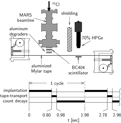
Figure 1: Schematic diagram of the end of MARS and the fast tape-transport system as well as a timing diagram for the experiment. The counting time for decays was generally 1 sec as indicated, but times of 2 and 4 sec were also used for the diagnosis of longer-lived contaminants.

II.1 $\gamma$ Efficiencies

The extremely precise absolute photopeak efficiency calibration of the HPGe detector is a critical component of this experiment. This efficiency has been carefully studied up to energies of 3.5 MeV as discussed in Refs. Hardy et al. (2002); Helmer et al. (2003, 2004). Over the range of $50-1400$ keV, Ref. Helmer et al. (2003) discusses how the absolute efficiency has been calibrated to $\pm 0.2\%$, and Ref. Helmer et al. (2004) uses a combination of measurements and calculations using the Cyltran Halbleib et al. (1992) Monte Carlo code to extend the efficiency curve from $1.4-3.5$ MeV to $\pm 0.4\%$ precision. For this work, the highest energy $\gamma$ rays observed are at $7.2$ MeV, requiring us to further extend the photopeak efficiency curve. Our adopted curve and its extrapolation, shown in the top panel of Fig. 2, is calculated using the the same Cyltran program used in Refs. Hardy et al. (2002); Helmer et al. (2003, 2004). Note that above 3.5 MeV, the efficiency curve is no longer linear on the log-log plot as a simple extrapolation might suggest, instead falling off more quickly. We additionally checked this extrapolation against an independent calculation based on the Monte Carlo radiation transport code Penelope Sempau et al. (1997). As can be seen in the bottom panel of Fig. 2, there is excellent agreement between the two calculated photopeak efficiencies over the range of energies observed in this work. As the figure also indicates, we increase the uncertainties in the efficiency curve, adopting conservative uncertainties of $\pm 1$% from 3.5–5 MeV, and $\pm 5\%$ above 5 MeV.  The differences between the Cyltran and Penelope extrapolated efficiency curves are well within these uncertainty ranges.

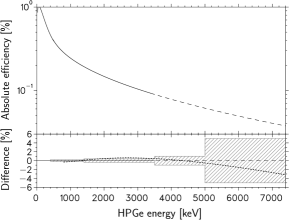
Figure 2: Top: the adopted absolute photopeak efficiency curve of the HPGe used in this work. The solid line is the measured efficiency up to 3.5 MeV from Refs. Hardy et al. (2002); Helmer et al. (2003, 2004), while the dashed line above 3.5 MeV represents an extrapolation based on Cyltran calculations. Bottom: percent difference of a Penelope simulation minus the adopted curve (dotted line) and the assigned uncertainties to the efficiency curve used in the present analysis (hatched region).

We have investigated the effects of summing in the HPGe detector using our Monte Carlo simulations. A small but non-negligible factor arises from Compton summing of $\gamma$ rays that scatter off various volumes. This makes knowing the total efficiency for $\gamma$ detection necessary, although the precision does not need to be very stringent because this summing with photopeak events is a small correction. However, accurately quantifying the effects of summing is difficult due to the large volume needed for tracking photons that may scatter from any of the surrounding elements. Our simulations where the geometry contained only detailed descriptions of the detectors and Mylar tape (i.e. neglecting the table, the floor, the walls, etc.) underestimates this summing effect. Rather than attempting to include the many potentially important scattering surfaces, we chose to perform Penelope simulations with our geometry encased by an Aluminum cylinder knowing that this surely overestimates the effect. The result of simulations using these two geometries is shown in Fig. 3 where differences as large as a factor of two arise at lower energies. We take the total efficiency to be halfway between these two simulated curves, with an uncertainty that spanned the results of both. This results in a large uncertainty in the total efficiency but since the Compton summing with photopeaks is a small correction, this conservative estimate does not limit our determination of the $\gamma$ branches.

We also investigated the possible effects of $\gamma$-ray angular correlations, which may affect the probability of a photopeak event summing with the photopeak from another cascade $\gamma$. The only cases that would result in a non-zero $\gamma$-$\gamma$ correlation are $1^{+}\!\!\rightarrow 2^{+}\!\!\rightarrow 0^{+}$ cascades; we tested both $E2$ and $M1$ transition types and found that independent of the transition type, $\gamma$-$\gamma$ angular correlations do not lead to any additional summing in our geometry.

Figure 3: Total efficiency of the HPGe as simulated by Penelope. The filled circles represent the simulated points with our basic geometry (detectors and Mylar tape) while the open circles show the results when our basic geometry is encased in an Aluminum cylinder. The dashed lines going through each is a 4^th order polynomial fit, and the solid central line is the average of the two which we take to be our total efficiency curve. We assign an uncertainty that spans the result of both simulations. We used these curves to determine systematic uncertainties associated with summing in our detectors.

II.2 $Q_{EC}$ and the $\beta$ Efficiency

The mass excess of ³²Cl is obtained from our averaging Refs. Wrede et al. (2010); Kankainen et al. (2010); Audi et al. (2003) to get $\mathrm{ME}(^{32}\mathrm{Cl})=-13334.60(57)$ keV, and $\mathrm{ME}(^{32}\mathrm{S})=-26015.535(2)$ keV is taken from Ref. Shi et al. (2005). Taken together, the decay energy is $Q_{EC}=12680.9(6)$ keV.  Although the fraction of events below the finite $E_{\beta}$ threshold of $40$ keV in the plastic scintillator is expected to have a weak dependence on the $\beta$ end-point energy, in principle the $\beta$ efficiency depends on $Q_{\beta}$. To investigate this effect, Penelope simulations were used to determine the $\beta$ efficiency of the plastic scintillator. A linear fit of the mean $\beta$ efficiency for the entire $\beta$ spectrum versus $\beta$ end-point energy yielded an efficiency that was consistent with being flat over the $4-12$-MeV range of end-points relevant for this decay: $\eta(Q_{\beta})=[32.32(41)-0.022(45)Q_{\beta}]\%$.

III Data analysis

Figure 4 shows the spectrum from the resistive-readout position-sensitive Silicon detector at the focal plane of MARS.  This logarithmic 2D plot shows that the most significant contaminations in the beam prior to our closing the purifying slits were ³⁰S and ³¹S, with ³²Cl making up $\approx 86\%$ of the beam at the focal plane of MARS.   The ³¹S contamination was minimized by closing the vertical slits at the focal plane of MARS as indicated in the figure, reducing it from $\approx 3\%$ to $\approx 0.4\%$. The slits had little effect at removing the ³⁰S contamination, however, as it lies in the same vertical band as the ³²Cl. The purity of the beam at the focal plane of MARS with the vertical slits in place was $\approx 89\%$. As mentioned previously, the ^30,31S contaminations were further reduced by the degraders, which were chosen to maximize the implantation of ³²Cl in the centre of the Mylar tape. The purity of the beam implanted in the tape was improved by another couple of percent to $\approx 91\%$ ³²Cl with ³⁰S the largest contaminant at $\approx 7.5\%$. Note that we could have obtained a higher purity at the cost of reducing the rate; however, since the $\gamma$ energies of the contaminants do not overlap the ³²Cl lines, we chose to maximize the rate.

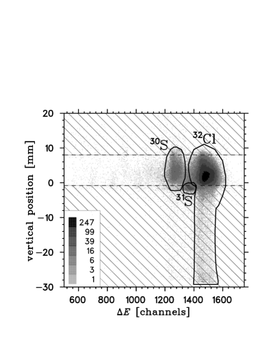
Figure 4: Identification of the ion beam at the focal plane of MARS, before the purifying slits in the vertical position were moved to the closed positions (indicated by the hatched areas). The region labeled ³²Cl represents 86% of all events in the spectrum, which was increased to 89% once the slits were in place. The tails in the vertical position are a result of incomplete charge collection in the resistive-readout Silicon $\Delta E$ detector.

The plot in Fig. 5 shows the time difference between $\beta$ particles detected in the scintillator and $\gamma$-rays observed in the HPGe detector plotted against the $\gamma$ energy. One clearly sees a strong peak at $t_{\beta}-t_{\gamma}\approx 475$ ns. In addition to the expected walk at low $\gamma$ energies (below 511 keV), a smaller 2^nd peak around 600 ns in the timing is visible; although the source of this peak is not fully understood, the $\gamma$ spectrum gated on just it proves that these are good events. We therefore included it in the analysis and defined a time gate between $430$ and $800$ ns to select real coincidences (the dashed horizontal lines in Fig. 5). The rest of the timing spectrum defines another window which selects accidental coincidences. The $E_{\gamma}$ projection of Fig. 5 shows two curves: the top one represents the projection of the real-coincidence window, and the lower one represents the accidental coincidences. The lower one, properly normalized, was then used as a background spectrum to be included in our fitting function as described below. The real-coincidence window position and size were varied significantly to check for potential systematic errors. This procedure yielded results with no significant sensitivity to the particular window used, as long as it covered the range containing all of the real coincidences.

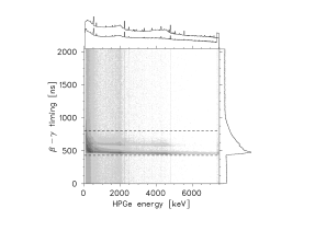
Figure 5: Logarithmic 2D plot of the $\gamma$ energy versus the timing between the $\beta$ and $\gamma$. Accidental coincident events were defined to have $t_{\beta\gamma}\leq 430$ ns or $t_{\beta\gamma}\geq 800$ ns. The lower curve of the projection of the HPGe energy represents these background events (scaled according to the cut-window size). The upper projection is the good events with $430~{}\mathrm{ns}<t_{\beta\gamma}<800$ ns.

Figure 6 shows the $\gamma$ spectrum observed in the HPGe detector in hardware coincidence with a $\beta$ signal in the scintillator. This is the same as the upper projection of Fig. 5 but with finer binning. Except for a strong peak at 677 keV from the decay of ³⁰S nearly every statistically significant peak is associated with the decay of ³²Cl. One exception is at 2776 keV where $360\pm 50$ counts are seen which could not be identified based on the known levels in ³²S Ouellet and Singh (2011) nor with any contaminants. If this was, in fact, a product of the decay of ³²Cl, it would only represent a 0.1% $\gamma$-ray yield.

Figure 6: The $\gamma$ spectrum observed by the HPGe detector in coincidence with a $\beta$. Peaks are labeled with their energy, the symbol * or the symbol **, referring to the full energy, single-escape and double-escape peaks, respectively. Peaks not associated with ³²Cl have in addition a label indicating the parent nucleus. Decays from the 7001-keV isobaric analogue state are highlighted with boxed values. The only significant background peak is at 677 keV from the ³⁰S contamination.

A reassuring check of the cleanliness of our data and identification of the ³⁰S contamination is shown in Fig. 7. This shows a comparison of the lifetime of the two most intense peaks in the ³²Cl spectrum (2230 and 4771 keV) as well as the main peak (677 keV) from ³⁰S. Dead time and pile-up effects were assumed to be negligible corrections and are not included in these half-life curves. The fit was from 0.060 to 0.985 s after the activity was transferred to the counting station. The fit lifetime of 2230-keV $\gamma$ events is $0.3012(13)$ s which is consistent with the $0.300(5)$ s lifetime fit from 4771-keV events. Both of these results are in agreement with the accepted half-life of $0.298(1)$ s of Ref. Armini et al. (1968). For the 667-keV line from ³⁰S events, the Compton tail from higher-energy $\gamma$s from the shorter-lived ³²Cl represent a contamination to the ³⁰S curve. In order to remove their effect, the minimum time included in the fit range for ³⁰S was 1 sec, over three ³²Cl half-lives. The fit yielded the half-life in this case to be $1.169(34)$ s, in good agreement with the accepted value of $1.1786(45)$ s from Ref. Wilson et al. (1980). Other ³²Cl peaks did not have enough statistics to be able to confirm the consistency of their $t_{1/2}$ decay curves.

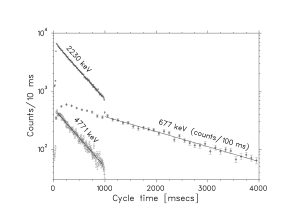
Figure 7: Number of counts as a function of time after the activity was transferred by the fast tape-transport system (points) and lifetime fits (solid lines). These decay spectra are gated on the two most prominent ³²Cl lines (2230 and 4771 keV) as well as the dominant contaminant, ³⁰S at 677 keV.   The ³²Cl peaks were fit to runs where events were counted for 1 s following transfer, and the longer-lived ³⁰S peak used runs where the count time was 4 s.

III.1 The $\gamma$ Peak Areas

In order to extract peak areas we used a fitting function consisting of four terms:

1. A Gaussian, $F_{\mathrm{Gauss}}=\frac{1}{\sqrt{2\pi}\sigma}\exp{\left(-\frac{(x-\mu)^{2}}{2\sigma^{2}}\right)}$, which corresponds to a $\delta$-function at the $\gamma$ peak channel number, $\mu$, convoluted with noise of width $\sigma$. Due to the sharp rise of this peak, we integrated the function over the ADC channel width, $\Delta x$, before comparing to the experimentally observed histogram. Thus the main peak of our fitting function is:

   $$F(x)=\frac{\frac{1}{2}\left[\mathrm{erf}\left(\frac{x-\mu+\Delta x/2}{\sqrt{2}\sigma}\right)-\mathrm{erf}\left(\frac{x-\mu-\Delta x/2}{\sqrt{2}\sigma}\right)\right]}{\Delta x},$$

   where $\mathrm{erf}$ is the error function.

2. A convolution of an exponential, $F_{\mathrm{exp}}=\exp{\left[-\lambda(x-\mu)\right]}$, with a Gaussian. Normalizing to unit area over the range zero to infinity, we define a low-energy tail function corresponding to incomplete charge collection as:

   $$T(x)=\frac{\lambda\ \exp\left(\frac{\lambda^{2}\sigma^{2}}{2}+\lambda(x-\mu)\right)\mathrm{erfc}\left(\frac{x-\mu+\lambda\sigma^{2}}{\sqrt{2}\sigma}\right)}{1+\mathrm{erf}\left(\frac{\mu}{\sqrt{2}\sigma}\right)-\exp\left(\frac{\lambda^{2}\sigma^{2}}{2}\!-\!\lambda\mu\right)\mathrm{erfc}\left(\frac{\lambda\sigma^{2}-\mu}{\sqrt{2}\sigma}\right)}.$$

   Here $\mathrm{erfc}(x)=1-\mathrm{erf}(x)$ is the complementary error function and $\lambda$ is the decay constant of the exponential.

3. A constant background, $F_{\mathrm{bkgd}}=b$.

4. The background histogram from the accidental coincidences in $\beta-\gamma$ timing, $F_{\mathrm{accid}}(x)$, as described previously.

In order that the total number of $\gamma$ signal events is a free parameter of the fits, we combined and normalized the terms so that our final fitting function was:

$$F_{\mathrm{fit}} =a_{\gamma}^{2}\left[(1-a_{\mathrm{tail}}^{2})F(x)+a_{\mathrm{tail}}^{2}T(x)\right]$$

$$\qquad\qquad\qquad\qquad+F_{\mathrm{bkgd}}+F_{\mathrm{accid}}(x).$$ (2)

In our model, the parameters $a_{\gamma}$ and $a_{\mathrm{tail}}$ are squared so that neither the normalization of the photopeak area nor the relative amplitude of the tail due to incomplete light collection are able to converge to a negative value when fitting very small amplitude or non-existant peaks. The total number of good $\gamma$ events in a peak is given by $N^{\gamma}=a_{\gamma}^{2}$ and the uncertainty is $\Delta N^{\gamma}=2a_{\gamma}\Delta a_{\gamma}$, where $\Delta a_{\gamma}$ is the statistical uncertainty returned from the fitting routine. Note that by defining the fitting function in this way, our statistical uncertainty in the number of $\gamma$ events includes any correlations with other parameters of the fit.

The $\gamma$ energies investigated included any transitions between states such that $E_{\gamma}>400$ keV.  The background from the Compton edge of the 511 keV peak compromised the sensitivity of searching for peaks below this energy. All fits were made using a FORTRAN code based on the Marquardt algorithm Marquardt (1963) for $\chi^{2}$ minimization. The program assumes Poisson statistics in the data (rather than Gaussian), and thus properly handles bins with very few counts. The data were divided into small blocks with equal number of total counts and analyzed individually. This procedure minimized the effects of gain variations since each data set was acquired over a limited range of time rather than over the whole run. Gain variations determined by the change in the fit centroid value were always below 0.05%; so in the end, the effects due to gain variations were negligible. The number of blocks of data varied for each peak depending on its intensity; for example, while fitting the high-statistics 2230-keV peak the data were divided into 170 blocks, while the much weaker 7189-keV peak had all of the data summed together into one histogram before fitting. When the data were divided into blocks for fitting, the areas were summed and uncertainties propagated to get the total number of counts. We note that this number is in statistical agreement with the result obtained when fitting the summed histogram, although in the latter case the $\chi^{2}$ was worse due to small drifts in the gain.

Figure 8 shows a typical fit to the 2230-keV peak. In general the fits were excellent, with very few converging with a confidence level (CL) far from the ideal 50%; the distribution of confidence levels has a mean of 30.8% and a standard deviation of 24.2%.

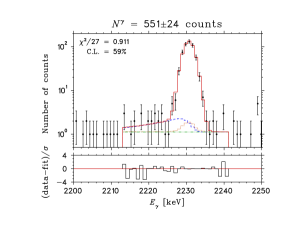
Figure 8: (Colour online) The top panel shows a typical fit, in this case to the 2230-keV peak, using the fitting function of Eq. (2). The dashed line is the tail, $T(x)$, from incomplete charge collection; the dotted is the accidental coincidences, $F_{\mathrm{accid}}$; the dash-dot line is a flat background; and the solid histogram is the total fitting function. The bottom panel shows the residual of the fit in terms of $\sigma$.

The energy calibration of the energy of our HPGe detector was made using: (a) the two most precisely known and strongest $\gamma$ de-excitations from levels in ³²S (2230.49(15) and 4281.51(26) keV from Ref. Babilon et al. (2002)); and (b) the three independent $\gamma$-rays from our main contaminant ³⁰S (667.01(3), 708.70(3) and 2342.2(1) keV Ouellet and Singh (2011)).

III.2 The $\beta$ and $\gamma$ Branches

Another FORTRAN code, also based on the Marquardt algorithm, was used to fit $\beta$ and $\gamma$ branches to the observed number of $\gamma$ events, $N^{\gamma}_{i,j}$, where $j$ represents the state to which the $i$^th state $\gamma$ decays. Letting $\beta_{i}$ represent the probability for the $\beta$ decay to proceed to state $i$, we normalize the $\beta$ branches such that

$$\sum\beta_{i}=1,$$ (3)

where $i$ is summed over all of the states considered in the analysis (see below). Similarly, we normalize the $\gamma$ branch probabilities, $\gamma_{i,j}$, from a given ³²S excited state $i$ to lower state $j$ as

$$\sum_{j<i}\gamma_{i,j}=1.$$ (4)

In terms of these branches, to first order the number of observed $\gamma$ rays is given by:

$$N^{\gamma}_{i,j}=N_{\mathrm{tot}}\left[\beta_{i}\eta_{i}+\sum_{k>i}\beta_{k}\eta_{k}\gamma_{k,i}\right]\gamma_{i,j}\epsilon_{i,j},$$ (5)

where the first term in the brackets arises from the $\beta$ transition directly to state $i$, and the second term represents the feeding from $\beta$ transitions to higher levels that $\gamma$ decay to state $i$. Here $N_{\mathrm{tot}}$ is the total number of decays (a free parameter in the fits since the total number of $\beta$’s was not precisely measured), $\epsilon_{i,j}$ is the photopeak efficiency of the HPGe detector at an energy $E_{i,j}$, and $\eta_{i}$ is the efficiency of the plastic scintillator to observe a $\beta$ with an end-point energy $Q_{i}$. Small corrections to Eq. (5) (included in the analysis but omitted here for clarity) are required to account for (a) summing with cascade $\gamma$s from above and below (which requires the total efficiency of the HPGe), and (b) summing with the $511$ annihilation radiation since this is a $\beta^{+}$ decay.

The nine lowest $(0,1,2)^{+}$ states observed by Détraz et al. Détraz et al. (1973) and Anderson et al. Anderson et al. (1966) along with the $(1.0^{+0.2}_{-0.5})\%$ ground state branch from Armini et al. Armini et al. (1968) represent most of the $\beta$ yield; however little is known above $7.2$ MeV of excitation energy. Some $\beta$-delayed proton and alpha decays have been observed Honkanen et al. (1979) to states above 8.7 MeV with particle energies as low as 762(5) keV, but this still leaves a $1.5$ MeV window of $Q$-value in which no $\beta$ transitions have been identified. This suggests that there is no appreciable $\beta$ feeding in this energy region; however, it does not rule out the possibility of a large number of weak $\beta$ transitions. Each of these transitions may be too small to be detected individually, but could cumulatively contribute a total $\beta$ strength of up to a few per cent. This “Pandemonium effect,” originally pointed out in Ref. Hardy et al. (1977), was raised again recently Hardy and Towner (2002) with regard to superallowed $\beta$ decay in $p,f$-shell nuclei. Following the approach advocated in these references, we use a shell-model calculation to compute the weak $\beta$ branches and include its predicted strength in the analysis. The model space used is the full $s,d$ shell with the effective interactions USD of Wildenthal Wildenthal (1984) and the two more recent updates USD-A and USD-B of Brown and Richter Brown and Richter (2006).

We include in our analysis of the branches and yields a total of $51$ excited states in ³²S.  Our shell-model calculation correctly predicts all of the $9$ lowest $(0,1,2)^{+}$ states with $E_{x}<7.2$ MeV reported in Détraz et al. Détraz et al. (1973). We find that the RMS deviations of the shell-model calculation from the known excitation energies Ouellet and Singh (2011) are quite good: 120 keV (USD), 209 keV (USD-A) and 172 keV (USD-B). This is a gratifying indication that the shell model is performing well in this $s,d$-shell nucleus. Even though selection rules prohibit $\beta$ decays to the six lowest $(3,4)^{\pm}$ states, they are included in the analysis when accounting for $\gamma$-ray de-excitations. The shell-model calculations identify approximately $40$ $\beta$ transitions to states whose excitation energies in ³²S lies between $7.485$ and $\approx 11.8$ MeV.  Unfortunately, the high density of states in this energy range makes a state-by-state comparison difficult, especially for the $2^{+}$ states. Based on the good correspondence of excitation energies and $\gamma$ de-excitation branches, we are able to identify $6$ of the shell-model states in this region with ones in the ENSDF Data Tables. None of the other $30$ shell-model states individually has a $\beta$-transition strength greater than $0.3\%$, but cumulatively they sum to $0.50\%$ in the USD, $0.69\%$ in the USD-A, and $0.55\%$ in the USD-B calculations. We include these weak $\beta$ strengths and de-excitation $\gamma$ rays predicted by the shell model in our overall analysis.

In the analysis, a $\beta$ branch could be deduced as long as there is at least one decay $\gamma$ ray lying within the 7.35 MeV energy range of our HPGe. The ground-state branch and higher excitation-energy shell-model-state branches that were not observed in this experiment were included in the analysis as missing strength. For the ground state, we take the branch to be $(1.0^{+0.2}_{-0.5})\%$ as determined by Armini et al. Armini et al. (1968), and the combination of all the unseen shell-model states at energies above 7.2 MeV is taken to be the average of the USD, USD-A and USD-B calculations with an uncertainty that spans the variation: $(0.60\pm 0.10)\%$. The $\alpha$-particle and proton-emitting states in the $8.7$ to $11.1$ MeV excitation energy range reported by Honkanen et al. Honkanen et al. (1979) are not separately included because their summed $\beta$ strength of $(0.080\pm 0.005)\%$ is significantly less than and no doubt already included in the missing strength predicted by the shell model.

IV Results

IV.1 Experimental Results

The excitation energies in ³²S, the $\beta$-decay branches and the $\log{ft}$ values determined in this work are shown in Table 1. The states up to 7.2 MeV each have multiple $\gamma$ rays which were observed in this work. Thus the $\gamma$ branches in these cases could be fit using the procedure described earlier. Furthermore, the fitting routine allowed us to treat the excitation energies of these states as free parameters, and fit the observed lines such that the $E_{x}$ values minimized the $\chi^{2}$ of the calculated $\gamma$ energies. For the highest three energy levels listed in Table 1, only one de-excitation $\gamma$ ray was observed; therefore, in these cases the $\gamma$ branches had to be taken from previous work Ouellet and Singh (2011), and the excitation energy had to be calculated solely on the one calibrated $\gamma$ ray that was observed.

In Table 2 we list the $\gamma$ branches for the states which have multiple $\gamma$ rays within our $7.35$ MeV energy range. The $\gamma$ energy in this table is calculated by first averaging the ENSDF Ouellet and Singh (2011) $E_{x}$’s with our own (the first two columns of Table 1) and then calculating the Doppler-corrected $E_{\gamma}$ based on the new excitation energies.

Table 1: Excitation energies in ³²S, deduced $\beta$ branches and the comparative half-lives of the decay of ³²Cl. The $0^{+}$ spin assignment of the $7637$- and $7921$-keV levels are determined from a comparison with our shell-model calculation. Not listed are the weakly-fed states between $7.4-11.8$ MeV predicted by the shell-model to have a total branch of $(0.60\pm 0.10)\%$.

$E_{x}$ in 32S [keV]

$\beta$ branch [%]

$\log ft$

$J^{\pi}_{n},T$

ENSDFa

This work

Average

Détraz et al.b

This work

Détraz et al.b

This work

$9207.55$±

$0.71$

$9204.7$±

$1.7$

$9207.1$±

$0.7$

$1^{+}_{5},1$

–

$0.22$±

$0.04^{+0.02}_{-0.09}$

–

4.

3${}_{-0.1}^{+0.4}$

$8125.40$±

$0.20$

–

$8125.40$±

$0.20$

$1^{+}_{4},1$

–

$<0.19$

–

$>5$.

$0$

$7921.0$±

$1.0$

$7924.3$±

$1.8$

$7921.8$±

$0.9$

$0^{+}_{5},0$

–

$0.033$±

$0.012^{+0.010}_{-0.004}$

–

5.

9${}_{-0.1}^{+0.3}$

$7637.0$±

$1.0$

–

$7637.0$±

$1.0$

$0^{+}_{4},0$

–

$<0.026$

–

$>6$.

$2$

$7535.7$±

$1.0$

$7535.3$±

$1.8$

$7535.6$±

$0.9$

$0^{+}_{3},1$

–

$0.185$±

$0.017^{+0.019}_{-0.003}$

–

5.

34${}_{-0.05}^{+0.04}$

$7190.1$±

$1.5$

$7190.5$±

$1.6$

$7190.3$±

$1.1$

$1^{+}_{3},0$

$0.9$±

$0.1$

$0.62$±

$0.05\!\pm\!0.01$

$4.90$±

$0.10$

4.

98${}_{-0.03}^{+0.04}$

$7115.3$±

$1.0$

$7114.7$±

$1.5$

$7115.1$±

$0.8$

$2^{+}_{5},1$

$0.5$±

$0.2$

$0.62$±

$0.04^{+0.00}_{-0.02}$

$5.1$±

$0.2$

5.

01$\pm$0.03

$7001.4$±

$0.4$

$7001.0$±

$1.3$

$7001.4$±

$0.4$

$1^{+}_{2},1$

$20.5$±

$2.0$

$22.47$±

$0.13^{+0.16}_{-0.12}$

$3.52$±

$0.04$

3.

500$\pm$0.004

$6666.1$±

$1.0$

$6665.4$±

$1.4$

$6665.9$±

$0.8$

$2^{+}_{4},0$

$1.8$±

$0.5$

$2.09$±

$0.07^{+0.01}_{-0.03}$

$4.72$±

$0.12$

4.

671${}^{+0.016}_{-0.014}$

$5548.5$±

$1.0$

$5548.3$±

$1.1$

$5548.4$±

$0.8$

$2^{+}_{3},0$

$4.1$±

$0.5$

$3.83$±

$0.07\!\pm\!0.09$

$4.77$±

$0.06$

4.

816${}^{+0.014}_{-0.012}$

$4695.3$±

$0.4$

$4695.5$±

$0.9$

$4695.3$±

$0.4$

$1^{+}_{1},0$

$6.8$±

$0.8$

$6.10$±

$0.08^{+0.03}_{-0.04}$

$4.81$±

$0.05$

4.

880${}^{+0.007}_{-0.006}$

$4281.8$±

$0.3$

$4281.9$±

$0.8$

$4281.81$±

$0.28$

$2^{+}_{2},0$

$3.1$±

$0.4$

$2.18$±

$0.08\!\pm\!0.02$

$5.45$±

$0.07$

5.

444${}^{+0.016}_{-0.015}$

$3778.4$±

$1.0$

$3778.1$±

$0.9$

$3778.3$±

$0.7$

$0^{+}_{2},0$

$2.6$±

$0.8$

$0.95$±

$0.07^{+0.01}_{-0.05}$

$5.48$±

$0.13$

5.

94${}_{-0.03}^{+0.04}$

$2230.57$±

$0.15$

$2230.4$±

$0.5$

$2230.56$±

$0.14$

$2^{+}_{1},0$

$60$±

$4$

$59.08$±

$0.18^{+0.39}_{-0.26}$

$4.49$±

$0.04$

4.

516${}^{+0.002}_{-0.003}$

ground state

$0^{+}_{1},0$

not measuredc

not measuredd

aRef. Ouellet and Singh (2011).

bRef. Détraz et al. (1973).

cFixed to $1.0^{+0.2}_{-0.5}\%$ from Armini, et al. Armini et al. (1968).

dCalculated to be $6.7^{+0.2}_{-0.1}$.

Table 2: $\gamma$-decay branches, in percent, for excited states in ³²S and comparison to the currently accepted values in ENSDF Ouellet and Singh (2011). The 2230.48(14) keV $2^{+}_{1}$ transition to the $0^{+}_{1}$ ground state is assumed to be 100% since there are no other known levels to which the $2^{+}_{1}$ state may decay. The energies of the $\gamma$ rays are calculated based on the adopted energy levels, i.e. the average of our work and ENSDF, the third column in Table 1 and shown in Fig. 9.

Transition	$E_{\gamma}$ [keV]	ENSDF				Present work			Transition	$E_{\gamma}$ [keV]	ENSDF				Present work
$1^{+}_{3}\rightarrow 2^{+}_{3}$	$1641.8\pm 1.3$					$<6$.	$7$		$2^{+}_{4}\rightarrow 2^{+}_{3}$	$1117.4\pm 1.1$					$<1$.	$1$
$1^{+}_{1}$	$2494.9\pm 1.1$		$<42$			$2$.	$6\!\pm\!2.1^{+0.1}_{-0.7}$		$1^{+}_{1}$	$1970.5\pm 0.9$		$14$	$\pm 2$		$7$.	$3\!\pm\!1.8^{+0.0}_{-0.2}$
$2^{+}_{2}$	$2908.4\pm 1.1$		$<35$			$<3$.	$4$		$2^{+}_{2}$	$2384.0\pm 0.9$		$<7$			$3$.	$7\!\pm\!0.9^{+0.0}_{-0.3}$
$0^{+}_{2}$	$3411.9\pm 1.3$		$<55$			$19$.	$5\!\pm\!2.7^{+0.2}_{-1.1}$		$0^{+}_{2}$	$2887.5\pm 1.0$		$49$	$\pm 5$		$46$.	$7\!\pm\!1.6^{+0.7}_{-0.2}$
$2^{+}_{1}$	$4959.3\pm 1.1$		$59$	$\pm 12$		$50$.	$8\!\pm\!3.8^{+0.8}_{-1.4}$		$2^{+}_{1}$	$4435.0\pm 0.8$		$37$	$\pm 4$		$39$.	$6\!\pm\!1.6^{+0.4}_{-0.7}$
$0^{+}_{1}$	$7189.4\pm 1.1$		$41$	$\pm 12$		$27$.	$1\!\pm\!2.9^{+2.0}_{-0.8}$		$0^{+}_{1}$	$6665.1\pm 0.8$		$<3$			$2$.	$3\!\pm\!0.8^{+0.3}_{-0.4}$
									$2^{+}_{3}\rightarrow 1^{+}_{1}$	$853.1\pm 0.8$					$0$.	$65\!\pm\!0.20\!\pm\!0.03$
									$2^{+}_{2}$	$1266.6\pm 0.8$		$<1$			$0$.	$86\!\pm\!0.30^{+0.12}_{-0.02}$
$2^{+}_{5}\rightarrow 2^{+}_{3}$	$1566.6\pm 1.1$					$<4$.	$6$		$0^{+}_{2}$	$1770.1\pm 1.0$		$<1$			$3$.	$3\!\pm\!0.6\!\pm\!0.1$
$1^{+}_{1}$	$2419.7\pm 0.9$		$9$	$\pm 1$		$9$.	$0\!\pm\!2.0^{+0.1}_{-1.0}$		$2^{+}_{1}$	$3317.7\pm 0.8$		$60$	.0$\pm$1.5		$59$.	$2\!\pm\!0.8^{+1.1}_{-0.9}$
$2^{+}_{2}$	$2833.2\pm 0.9$		$3$	$\pm 1$		$3$.	$0\!\pm\!2.0^{+0.6}_{-0.4}$		$0^{+}_{1}$	$5547.9\pm 0.7$		$40$	.0$\pm$1.5		$36$.	$1\!\pm\!0.7^{+1.0}_{-1.1}$
$0^{+}_{2}$	$3336.7\pm 1.1$		$3$	$\pm 2$		$5$.	$8\!\pm\!2.2^{+0.0}_{-0.3}$
$2^{+}_{1}$	$4884.1\pm 0.8$		$83$	$\pm 2$		$79$.	$3\!\pm\!3.9^{+1.2}_{-0.5}$		$1^{+}_{1}\rightarrow 2^{+}_{2}$	$413.5\pm 0.5$		$<0$	$.6$		$<0$.	$28$
$0^{+}_{1}$	$7114.3\pm 0.8$		$2$	.9$\pm$0.5		$<4$.	$6$		$0^{+}_{2}$	$917.1\pm 0.8$		$<0$	$.4$		$0$.	$50\!\pm\!0.14^{+0.01}_{-0.04}$
									$2^{+}_{1}$	$2464.7\pm 0.4$		$61$	.0$\pm$1.0		$63$.	$3\!\pm\!0.5^{+0.2}_{-0.1}$
									$0^{+}_{1}$	$4695.0\pm 0.4$		$39$	.0$\pm$1.0		$36$.	$2\!\pm\!0.5^{+0.1}_{-0.2}$
$1^{+}_{2}\rightarrow 2^{+}_{3}$	$1452.9\pm 0.8$					$1$.	$23\!\pm\!0.08\!\pm\!0.01$		$2^{+}_{2}\rightarrow 0^{+}_{2}$	$503.5\pm 0.7$		$<0$	$.3$		$<1$.	$5$
$1^{+}_{1}$	$2305.9\pm 0.5$		$<1$			$0$.	$61\!\pm\!0.10\!\pm\!0.03$		$2^{+}_{1}$	$2051.2\pm 0.3$		$13$	.0$\pm$0.5		$16$.	$1\!\pm\!0.9^{+0.1}_{-0.4}$
$2^{+}_{2}$	$2719.4\pm 0.5$		$<2$			$2$.	$37\!\pm\!0.08^{+0.01}_{-0.07}$		$0^{+}_{1}$	$4281.5\pm 0.3$		$87$	.0$\pm$0.5		$83$.	$5\!\pm\!1.1^{+0.3}_{-0.1}$
$0^{+}_{2}$	$3222.9\pm 0.8$		$9$	$\pm 5$		$3$.	$92\!\pm\!0.12^{+0.05}_{-0.02}$
$2^{+}_{1}$	$4770.4\pm 0.4$		$91$			$91$.	$63\!\pm\!0.19^{+0.06}_{-0.04}$		$0^{+}_{2}\rightarrow 2^{+}_{1}$	$1547.7\pm 0.7$		$99$	$.965$		$98$.	$6\!\pm\!0.8^{+0.2}_{-0.0}$
$0^{+}_{1}$	$7000.5\pm 0.4$		$<2$			$0$.	$25\!\pm\!0.07\!\pm\!0.01$		$0^{+}_{1}$	$3778.0\pm 0.7$		$0$	.035$\pm$0.006		$1$.	$4\!\pm\!0.8^{+0.0}_{-0.2}$

Figure 9 graphically depicts the results listed in Tables 1 and 2. The figure also includes within it the references to previous results which were used in the analysis. For example, the $\gamma$ ray from the $1_{5}^{+}$ state at 9206 keV was outside the energy range of our HPGe, so we took its $\gamma$ de-excitation branching ratio from the ENSDF Data Tables in order to fit the $\beta$ branch based on the observed $\gamma$ ray to the $2^{+}_{1}$ first excited state.

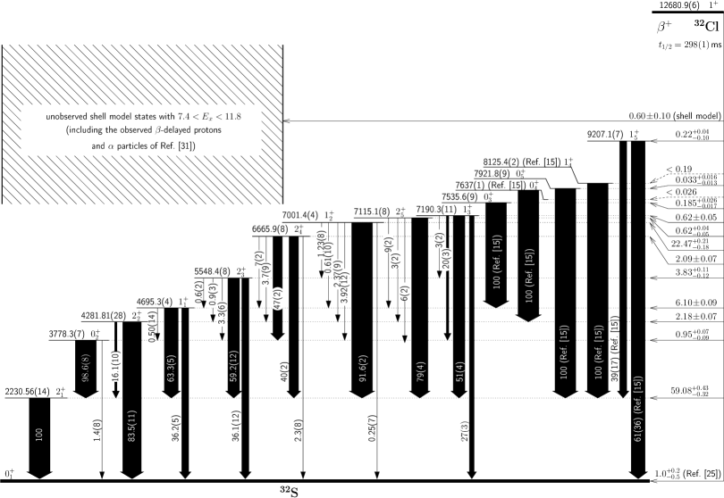
Figure 9: $\beta^{+}$ decay scheme for ³²Cl, summarizing the $\gamma$ and $\beta$ branches in Tables 1 and 2 determined from this work. All branches are expressed in percent. The excitation energies are the weighted average of the present work and the accepted values from ENSDF Ouellet and Singh (2011) (third column of Table 1).

In both Tables 1 and 2, the first uncertainty in the branches is statistical and the second is systematic. The sources of systematic error considered include: the cuts made on the data (the $\beta$/HI ratio, the $\beta$–$\gamma$ timing windows for real versus accidental coincidences, and the start/stop of the counting time following transfer of the activity); the uncertainty in the $\gamma$ photopeak areas and total efficiencies; the $\beta$ efficiency; the effective interaction of the shell model used for weakly-fed states above 7.2 MeV; including/excluding the ENSDF $\gamma$ branches for higher levels (and varying them by their uncertainties when included); and the ${}^{+0.2}_{-0.5}\%$ uncertainty in the ground state branch. For the $\gamma$ branches in Table 2, the sum of the quoted probabilities for decay from a given excited state in ³²S is not necessarily 100%, i.e. contrary to Eq. (4), it may seem that $\sum_{j<i}\gamma_{i,j}\leq 1$; this is because of possible–but not statistically significant–peaks where the data only allows us to place limits on the branch. As with the $\gamma$ yields discussed below, a branch is quoted only if the area of a $\gamma$-ray peak in the HPGe was larger than its total uncertainty. If this condition is not satisfied, we instead quote an upper limit on the branch at the 90% C.L.  For example, the $2^{+}_{5}$ state at 7115 keV has four statistically significant branches which have a combined probability of only $97.1\pm 5.3^{+1.3}_{-1.2}$%. For the other two branches, the fit converged to results that were consistent with zero and for which only upper limits may be quoted: $1.2\!\pm\!2.3^{+0}_{-0.5}\%$ ($2^{+}_{3}$) and $1.7\!\pm\!2.0^{+0.6}_{-0.1}\%$ ($0^{+}_{1}$). All together, including these statistically insignificant transition strengths, the total probability is 100%; the “missing” 2.9% in Table 2 for the decay from the $2^{+}_{5}$ state is potentially within transitions which are below our detection sensitivity. Note, however, that the $1$-$\sigma$ upper limit on the sum of the statistically significant branches includes 100%.

With the $\beta$ and $\gamma$ branches established, we are able to calculate the $\gamma$ yields. The reason we present the yields after the discussion of the branches is because of the small summing corrections which depend on the branching ratios. The results are listed in Table 3 where we again compare the excitation energies to ENSDF Ouellet and Singh (2011) and the yields to the work of Détraz et al. Détraz et al. (1973).

Table 3: Yields of $\gamma$-rays following the $\beta$ decay of ³²Cl. All values are in percent, and limits correspond to the 90% confidence level. The overall normalization is fixed such that the transition to the ground state is consistent with $1.0^{+0.2}_{-0.5}\%$ as reported by Armini, et al. Armini et al. (1968) and includes the $(0.60\pm 0.10)\%$ unobserved, weakly-fed shell-model states in the energy range of $7.4-11.8$ MeV.

$E_{\gamma}$ [keV]

$\gamma$ yield [%]

Transition

ENSDFa

This work

Détraz et al.b

This work

$7189.2$±

$1.5$

$7189.8$±

$1.2$

$1^{+}_{3}$

$(7190)$

$\rightarrow$

$0^{+}_{1}$

$(\mathrm{g.s.})$

$0.41$±

$0.10$

$0.169^{+0.024}_{-0.020}$

$7114.5$±

$1.0$

$2^{+}_{5}$

$(7115)$

$\rightarrow$

$0^{+}_{1}$

$(\mathrm{g.s.})$

$<0.029$

$7000.6$±

$0.4$

$7001.4$±

$1.6$

$1^{+}_{2}$

$(7001)$

$\rightarrow$

$0^{+}_{1}$

$(\mathrm{g.s.})$

$0.057\!\pm\!0.016$

$6976.2$±

$0.7$

$6973.5$±

$1.3$

$1^{+}_{5}$

$(9208)$

$\rightarrow$

$2^{+}_{1}$

$(2230)$

$0.098\pm 0.018$

$6665.4$±

$1.0$

$6665.8$±

$2.1$

$2^{+}_{4}$

$(6666)$

$\rightarrow$

$0^{+}_{1}$

$(\mathrm{g.s.})$

$0.048^{+0.018}_{-0.019}$

$5894.2$±

$0.2$

$1^{+}_{4}$

$(8125)$

$\rightarrow$

$2^{+}_{1}$

$(2230)$

$<0.027$

$5689.9$±

$1.0$

$5693.3$±

$1.3$

$0^{+}_{5}$

$(7921)$

$\rightarrow$

$2^{+}_{1}$

$(2230)$

$0.033^{+0.014}_{-0.013}$

$5548.0$±

$1.0$

$5548.9$±

$0.9$

$2^{+}_{3}$

$(5549)$

$\rightarrow$

$0^{+}_{1}$

$(\mathrm{g.s.})$

$1.6$±

$0.3$

$1.50^{+0.08}_{-0.09}$

$4959.1$±

$1.5$

$4959.6$±

$0.8$

$1^{+}_{3}$

$(7190)$

$\rightarrow$

$2^{+}_{1}$

$(2230)$

$0.32\!\pm\!0.04$

$4884.3$±

$1.0$

$4883.7$±

$0.8$

$2^{+}_{5}$

$(7115)$

$\rightarrow$

$2^{+}_{1}$

$(2230)$

$0.45$±

$0.20$

$0.504^{+0.031}_{-0.032}$

$4770.4$±

$0.4$

$4770.8$±

$0.8$

$1^{+}_{2}$

$(7001)$

$\rightarrow$

$2^{+}_{1}$

$(2230)$

$20.5$±

$2.0$

$20.62^{+0.20}_{-0.17}$

$4694.9$±

$0.4$

$4695.6$±

$0.8$

$1^{+}_{1}$

$(4695)$

$\rightarrow$

$0^{+}_{1}$

$(\mathrm{g.s.})$

$2.8$±

$0.6$

$2.42\!\pm\!0.05$

$4435.2$±

$1.0$

$4435.5$±

$0.8$

$2^{+}_{4}$

$(6666)$

$\rightarrow$

$2^{+}_{1}$

$(2230)$

$0.8$±

$0.2$

$0.83\!\pm\!0.06$

$4281.5$±

$0.3$

$4282.0$±

$0.7$

$2^{+}_{2}$

$(4282)$

$\rightarrow$

$0^{+}_{1}$

$(\mathrm{g.s.})$

$2.6$±

$0.1$

$2.42\!\pm\!0.06$

$3778.2$±

$1.0$

$3777$±

$4$

$0^{+}_{2}$

$(3778)$

$\rightarrow$

$0^{+}_{1}$

$(\mathrm{g.s.})$

$0.044\!\pm\!0.025$

$3411.5$±

$1.8$

$3412.2$±

$0.7$

$1^{+}_{3}$

$(7190)$

$\rightarrow$

$0^{+}_{2}$

$(3778)$

$0.122\!\pm\!0.019$

$3355.0$±

$1.0$

$0^{+}_{4}$

$(7637)$

$\rightarrow$

$2^{+}_{2}$

$(4282)$

$<0.026$

$3336.7$±

$1.4$

$3339.7$±

$1.2$

$2^{+}_{5}$

$(7115)$

$\rightarrow$

$0^{+}_{2}$

$(3778)$

$0.037\!\pm\!0.015$

$3317.7$±

$1.0$

$3317.9$±

$0.6$

$2^{+}_{3}$

$(5549)$

$\rightarrow$

$2^{+}_{1}$

$(2230)$

$2.5$±

$0.4$

$2.46\!\pm\!0.05$

$3222.8$±

$1.1$

$3222.4$±

$0.6$

$1^{+}_{2}$

$(7001)$

$\rightarrow$

$0^{+}_{2}$

$(3778)$

$0.881^{+0.029}_{-0.027}$

$2908.2$±

$1.5$

$1^{+}_{3}$

$(7190)$

$\rightarrow$

$2^{+}_{2}$

$(4282)$

$<0.022$

$2887.6$±

$1.4$

$2887.0$±

$0.5$

$2^{+}_{4}$

$(6666)$

$\rightarrow$

$0^{+}_{2}$

$(3778)$

$1.0$±

$0.4$

$0.976^{+0.028}_{-0.025}$

$2840.3$±

$1.1$

$2839.7$±

$0.5$

$0^{+}_{3}$

$(7536)$

$\rightarrow$

$1^{+}_{1}$

$(4695)$

$0.185\!\pm\!0.018$

$2833.4$±

$1.0$

$2832.4$±

$1.5$

$2^{+}_{5}$

$(7115)$

$\rightarrow$

$2^{+}_{2}$

$(4282)$

$0.019\!\pm\!0.013$

$2719.5$±

$0.5$

$2719.0$±

$0.5$

$1^{+}_{2}$

$(7001)$

$\rightarrow$

$2^{+}_{2}$

$(4282)$

$0.533^{+0.019}_{-0.024}$

$2494.7$±

$1.6$

$2495.2$±

$2.3$

$1^{+}_{3}$

$(7190)$

$\rightarrow$

$1^{+}_{1}$

$(4695)$

$0.016\!\pm\!0.014$

$2464.6$±

$0.4$

$2464.4$±

$0.5$

$1^{+}_{1}$

$(4695)$

$\rightarrow$

$2^{+}_{1}$

$(2230)$

$4.0$±

$0.4$

$4.24\!\pm\!0.05$

$2419.9$±

$1.1$

$2417.7$±

$0.6$

$2^{+}_{5}$

$(7115)$

$\rightarrow$

$1^{+}_{1}$

$(4695)$

$0.057^{+0.013}_{-0.015}$

$2384.2$±

$1.0$

$2383.3$±

$0.5$

$2^{+}_{4}$

$(6666)$

$\rightarrow$

$2^{+}_{2}$

$(4282)$

$0.077^{+0.019}_{-0.021}$

$2306.0$±

$0.6$

$2305.2$±

$0.5$

$1^{+}_{2}$

$(7001)$

$\rightarrow$

$1^{+}_{1}$

$(4695)$

$0.137\!\pm\!0.023$

$2230.49$±

$0.15$

$2230.2$±

$0.4$

$2^{+}_{1}$

$(2230)$

$\rightarrow$

$0^{+}_{1}$

$(\mathrm{g.s.})$

$92$±

$4$

$91.9^{+0.6}_{-0.4}$

$2051.2$±

$0.3$

$2050.7$±

$0.4$

$2^{+}_{2}$

$(4282)$

$\rightarrow$

$2^{+}_{1}$

$(2230)$

$0.47\!\pm\!0.04$

$1970.7$±

$1.1$

$1969.3$±

$0.6$

$2^{+}_{4}$

$(6666)$

$\rightarrow$

$1^{+}_{1}$

$(4695)$

$0.15\!\pm\!0.04$

$1770.0$±

$1.4$

$1769.6$±

$0.4$

$2^{+}_{3}$

$(5549)$

$\rightarrow$

$0^{+}_{2}$

$(3778)$

$0.136\!\pm\!0.026$

$1641.6$±

$1.8$

$1^{+}_{3}$

$(7190)$

$\rightarrow$

$2^{+}_{3}$

$(5549)$

$<0.04$

$1566.8$±

$1.4$

$2^{+}_{5}$

$(7115)$

$\rightarrow$

$2^{+}_{3}$

$(5549)$

$<0.030$

$1547.8$±

$1.0$

$1547.1$±

$0.4$

$0^{+}_{2}$

$(3778)$

$\rightarrow$

$2^{+}_{1}$

$(2230)$

$3.6$±

$0.6$

$3.155^{+0.040}_{-0.036}$

$1452.9$±

$1.1$

$1451.8$±

$0.4$

$1^{+}_{2}$

$(7001)$

$\rightarrow$

$2^{+}_{3}$

$(5549)$

$0.276\!\pm\!0.019$

$1266.7$±

$1.0$

$1265.7$±

$0.6$

$2^{+}_{3}$

$(5549)$

$\rightarrow$

$2^{+}_{2}$

$(4282)$

$<0.036\!\pm\!0.013$

$1117.6$±

$1.4$

$2^{+}_{4}$

$(6666)$

$\rightarrow$

$2^{+}_{3}$

$(5549)$

$<0.022$

$916.9$±

$1.1$

$915.8$±

$0.5$

$1^{+}_{1}$

$(4695)$

$\rightarrow$

$0^{+}_{2}$

$(3778)$

$0.034\!\pm\!0.009$

$853.2$±

$1.1$

$851.8$±

$0.5$

$2^{+}_{3}$

$(5549)$

$\rightarrow$

$1^{+}_{1}$

$(4695)$

$0.027\!\pm\!0.008$

$503.4$±

$1.0$

$2^{+}_{2}$

$(4282)$

$\rightarrow$

$0^{+}_{2}$

$(3778)$

$<0.04$

$413.5$±

$0.5$

$1^{+}_{1}$

$(4695)$

$\rightarrow$

$2^{+}_{2}$

$(4282)$

$<0.019$

aCalculated from the adopted levels of Ref. Ouellet and Singh (2011).

bRef. Détraz et al. (1973).

There is generally good agreement with the results of Détraz et al., although we find significantly less strength in the $\beta$ branches to the 3.78 and 4.28 MeV levels. We attribute this discrepancy to the fact that many of the higher levels not considered in Ref. Détraz et al. (1973) $\gamma$ de-excite through these levels; thus though our $\gamma$-ray yields for these states are in good agreement, our $\gamma$-ray feeding from higher levels results in a smaller deduced $\beta$ branch for these states. Another difference from Détraz et al. is seen with the 7190 keV $1^{+}_{3}$ level where we see less than half as much $\gamma$ yield, and find a $\beta$ branch that is 30% smaller. It is difficult to comment on this discrepancy since an efficiency curve is not provided in Ref. Détraz et al. (1973).

The shell-model predictions of the $\beta$ branches for the five highest energy levels of Table 1 are: 0.22(4)% (7536 keV); 0.05(4)% (7637 keV); 0.10(3)% (7921 keV); 0.06(1)% (8125 keV); and 0.06(1)% (9208 keV). The agreement is quite reasonable, where the only significant difference ($>2\sigma$) seen is in the branch to the 8125-keV level; here the shell model calculation predicts $\approx 3\times$ more strength than our limits allow for the branch to the 8125-keV state. Note that the sum of these branches in the shell model, $0.49(7)\%$, is in perfect agreement with the corresponding sum of the observed branches: $(0.51^{+0.10}_{-0.14})\%$. Given the high density of states in this energy range, it is a testament to the quality of the shell-model in this case that these branches are reproduced so well. It further justifies our use of the shell model to account for the Pandemonium effect as discussed earlier.

In addition to reducing the uncertainties in all of the branches/yields by approximately an order of magnitude, we have observed $22$ more $\gamma$ branches and three new $\beta$ branches compared to Détraz et al. Détraz et al. (1973). For the ten $\gamma$ and two $\beta$ transitions where we did not observe a statistically significant branch, a 90% CL limit is quoted.

IV.2 Comparison to Shell-Model Calculations

Shell-model calculations have been performed for the states involved in the $\beta$-decay of ³²Cl, which has a spin-parity of $1^{+}$. For transitions to $0^{+}$ and $2^{+}$ states in ³²S, the strength is pure Gamow-Teller whereas for the isobaric analogue transition, the decay is almost pure Fermi. Decays to non-analogue $1^{+}$ states can also include a Fermi component (via isospin mixing) and so for an experimental branch to one of these states, we can proceed in one of two ways:

1. make some assumptions about the Fermi contribution and deduce $|M(\mathrm{GT})|$.

2. make some assumptions about the Gamow-Teller contribution and deduce $|M(\mathrm{F})|$.

In the next section we discuss Gamow-Teller matrix elements after making some minimal assumptions about the Fermi contribution. We will compare our experimental $M(\mathrm{GT})$ values with shell-model computations to say something about the quality of the USD wave functions. Following this, we take the other approach by assuming that the USD values for $B(\mathrm{GT})$ are correct allowing us to deduce $B(\mathrm{F})$. In turn we can calculate an experimental value for the isospin-mixing parameter, $\delta_{C1}$, which we compare with theoretical calculations.

IV.2.1 Gamow-Teller matrix elements

Here we present a comparison of calculated versus experimental $B(\mathrm{GT})$’s. Because several of the transitions are quite retarded, with $\log{ft}$ values exceeding 5 (see Table 1), the spectrum shape may depart significantly from the allowed shape. To proceed, we use a shell-model calculation to compute the shape correction function $C(W)$ as described in the appendix of Ref. Hardy and Towner (2005b). We define an “exact” statistical rate function as

$$f_{\mathrm{exact}}=\int_{1}^{W_{0}}pW(W_{0}-W)^{2}\,F(Z,W)\,C(W)\,dW,$$ (6)

where $W=E_{e}/m_{e}$ is the electron total energy in electron rest-mass units, $W_{0}$ is the maximum value of $W$, $p=(W^{2}-1)^{1/2}$ is the electron momentum, $Z$ is the charge of the daughter nucleus, and $F(Z,W)$ is the Fermi function. The usual statistical rate function, $f$, as used for example in Table 1 to obtain $\log{ft}$ values, puts the shape correction function $C(W)$ to unity. Taking the Fermi strength to be zero for these non-analogue transitions, we obtain an experimental value for the GT strength from

$$B_{\mathrm{exp}}(\mathrm{GT})=\frac{2\mathcal{F}t^{0^{+}\!\!\rightarrow 0^{+}}}{f_{\mathrm{exact}}t(1+\delta_{R}^{\prime})},$$ (7)

and an associated experimental GT matrix element, $M_{\mathrm{exp}}(\mathrm{GT})$, defined by:

$$B_{\mathrm{exp}}(\mathrm{GT})=g_{A,\mathrm{eff}}^{2}|M_{\mathrm{exp}}(\mathrm{GT})|^{2}.$$ (8)

Because $f_{\rm exact}$ depends on the GT matrix element via $C(W)$, we use an iterative procedure which is explained below. In Eq. (7) we use $\mathcal{F}t^{0^{+}\!\!\rightarrow 0^{+}}=3071.81(83)$ s from the survey of Hardy and Towner Hardy and Towner (2009). The partial half-life, $t$, is calculated from the ³²Cl half-life of $t_{1/2}=298(1)$ ms Armini et al. (1968) and the branches, $R$, listed in Table 1, corrected for a small electron-capture fraction, $P_{\mathrm{EC}}$:

$$t=\frac{t_{1/2}}{R}\left(1+P_{\mathrm{EC}}\right).$$ (9)

The correction $\delta_{R}^{\prime}$ is the transition-dependent part of the radiative correction and is obtained from a standard QED calculation that depends on $Z$ and $W$. It is evaluated to order $\alpha$ and $Z\alpha^{2}$, with the order $Z^{2}\alpha^{3}$ terms estimated Sirlin (1967, 1987); Jaus and Rasche (1987); Czarnecki et al. (2004). Thus with the quantities on the right-hand side of Eq. (7) determined, an experimental $B_{\mathrm{exp}}(\mathrm{GT})$ value is obtained. This relates to the Gamow-Teller matrix element, $M_{\mathrm{exp}}(\mathrm{GT})$, as shown in Eq. (8). It requires knowledge of the ratio of the axial-vector to vector coupling constants, denoted $g_{A}$, for which an effective value is used, $g_{A,\mathrm{eff}}$ in the context of shell-model calculations in finite model spaces. In the $s,d$ shell, the systematic studies of Wildenthal and Brown Brown and Wildenthal (1985, 1987) have shown the effective value to be of order unity, so we take $g_{A,\mathrm{eff}}=1$.

In the shell model, the calculation of the Gamow-Teller matrix element is based on:

$$M(\mathrm{GT})=\sum_{\alpha,\beta}\langle f|a_{\alpha}^{{\dagger}}b_{\beta}|i\rangle\langle\alpha|\mathrm{GT}|\beta\rangle,$$ (10)

where $a_{\alpha}^{{\dagger}}$ creates a neutron in quantum state $\alpha$, $b_{\beta}$ annihilates a proton in quantum state $\beta$ and $\langle\alpha|\mathrm{GT}|\beta\rangle$ is the single-particle Gamow-Teller matrix element. The matrix element of $a_{\alpha}^{{\dagger}}b_{\beta}$ in the initial and final many-body states are known as the one-body density matrix elements (OBDME). The same OBDME used in the construction of the shape-correction function, $C(W)$, are also used in the shell-model evaluation of $M(\mathrm{GT})$. Our procedure is to scale one of these OBDME, recompute $C(W)$ and $f_{\mathrm{exact}}$, and obtain a new $M_{\mathrm{exp}}(\mathrm{GT})$ from Eq. (7). We then repeat the procedure, refining the scaling at each step until the theory input matches the experimental output. We found that it did not matter which USD calculation we started from, or which OBDME we scaled; the convergent result for the Gamow-Teller matrix element was always the same. Thus the method is quite stable.

Table 4: Deduced experimental Gamow-Teller matrix elements, $M_{\mathrm{exp}}(\mathrm{GT})$, in the decay of ³²Cl, and comparison with three shell-model calculations. The RMS deviations in the predicted $|M(\mathrm{GT})|$ compared to experiment are $0.073$ (USD), $0.068$ (USD-A) and $0.067$ (USD-B).

								Experiment		Theory $|M(\mathrm{GT})|$
$E_{x}$ in 32Sa		$J_{n}^{\pi},T$	$t$ [s]		$f_{\mathrm{exact}}\,^{b}$		$\delta_{R}^{\prime}~{}[\%]$	$|M(\mathrm{GT})|$		USD	USD-A	USD-B
$9207.1$±	$0.7$	$1_{5}^{+},1$	135	${}_{-22}^{+115}$	133	$.2\!\pm\!0.2$	$1.70(3)$	$0.58$	$\!\!\!\!{}^{+0.05}_{-0.15}$	$0.300$	$0.348$	$0.298$
$8125.4$±	$0.2$	$1_{4}^{+},1$	$>150$		689	$.2\!\pm\!2.7$	$1.55(3)$	$<0.20$		$0.123$	$0.146$	$0.134$
$7921.8$±	$0.9$	$0_{5}^{+},0$	900	${}_{-300}^{+600}$	879	$.5\!\pm\!1.3$	$1.52(3)$	$0.087$	$\pm 0.019$	$0.130$	$0.148$	$0.183$
$7637.0$±	$1.0$	$0_{4}^{+},0$	$>1200$		1261	$\pm 4$	$1.49(3)$	$<0.05$		$0.121$	$0.022$	$0.056$
$7535.6$±	$0.9$	$0_{3}^{+},1$	161	$\pm 18$	1392	$\pm 3$	$1.48(3)$	$0.164$	$\pm 0.009$	$0.193$	$0.165$	$0.192$
$7190.3$±	$1.1$	$1_{3}^{+},0$	48	$\pm 4$	2024	$\pm 4$	$1.44(3)$	$0.250$	$\pm 0.010^{c}$	$0.143$	$0.117$	$0.162$
$7115.1$±	$0.8$	$2_{5}^{+},1$	48	$\pm 3$	2232	$.4\!\pm\!2.4$	$1.44(3)$	$0.238$	$\pm 0.008$	$0.259$	$0.166$	$0.228$
$7001.4$±	$0.4$	$1_{2}^{+},1$	1	.327$\pm 0.012$	2413	$.0\!\pm\!1.7$	$1.42(3)$			$0.012$	$0.064$	$0.036$
$6665.9$±	$0.8$	$2_{4}^{+},0$	14	.3$\pm 0.5$	3411	$\pm 4$	$1.40(3)$	$0.353$	$\pm 0.006$	$0.428$	$0.273$	$0.365$
$5548.4$±	$0.8$	$2_{3}^{+},0$	7	.79$\pm 0.23$	8583	$\pm 7$	$1.30(3)$	$0.301$	$\pm 0.004$	$0.227$	$0.333$	$0.302$
$4695.3$±	$0.4$	$1_{1}^{+},0$	4	.89$\pm 0.07$	15702	$\pm 30$	$1.24(3)$	$0.281$	$\pm 0.002^{c}$	$0.280$	$0.309$	$0.346$
$4281.81$±	$0.28$	$2_{2}^{+},0$	13	.7$\pm 0.5$	21280	$\pm 10$	$1.22(3)$	$0.145$	$\pm 0.003$	$0.071$	$0.059$	$0.085$
$3778.3$±	$0.7$	$0_{2}^{+},0$	31	$\pm 3$	28009	$\pm 26$	$1.18(3)$	$0.083$	$\pm 0.003$	$0.076$	$0.137$	$0.077$
$2230.56$±	$0.14$	$2_{1}^{+},0$	0	.504$\pm 0.003$	67470	$\pm 40$	$1.11(3)$	$0.423$	$\pm 0.001$	$0.423$	$0.421$	$0.457$
ground state		$0_{1}^{+},0$	30	${}_{-5}^{+30}$	167900	$\pm 1600$	$0.94(3)$	$0.035$	$\!{}_{-0.010}^{+0.003}$	$0.004$	$0.089$	$0.024$
aThe average of currently accepted values and the present work, i.e. the third column of Table 1.
bThe error bar reflects both the uncertainty in the $Q$-value and the range obtained for different shell-model calculations of the shape-correction function, $C(W)$.
cFor these non-analogue $1^{+}$ transitions the experimental derived value is $\sqrt{B(\mathrm{F})+B(\mathrm{GT})}$, where the Fermi contribution originates from isospin mixing as discussed in the text. For the 4695-keV level, the Fermi contribution is theoretically expected to be very small, so the value quoted is likely a good estimate for $|M_{\mathrm{exp}}(\mathrm{GT})|$. For the 7190-keV level, the Fermi contribution is likely substantial, so a conservative estimate for $|M_{\mathrm{exp}}(\mathrm{GT})|$ is in the range $0<|M_{\mathrm{exp}}(\mathrm{GT})|<0.260$.

In Table 4 we list the partial half-lives, $t$, the statistical rate function $f_{\mathrm{exact}}$ at convergence, the radiative correction $\delta_{R}^{\prime}$, and the deduced experimental Gamow-Teller matrix element. We also list the theoretical values from three shell-model calculations with effective interactions USD, USD-A and USD-B, now without any of the adjustments to the OBDME discussed above. Thus, Table 4 compares $M_{\mathrm{exp}}(\mathrm{GT})$ values with theoretical expectations. The comparison is very favourable with the RMS difference $\approx 0.07$. Where the matrix element is quite large, say $M(\mathrm{GT})>0.2$, theory does exceedingly well. For retarded transitions with $M(\mathrm{GT})<0.2$, theory does not perform as well, but here the small values are a consequence of cancellations among shell-model amplitudes which are much harder to get precisely right. The same comparison is presented in Fig. 10, where the integrated $B(\mathrm{GT})$ values are displayed as a function of excitation energy. As has been found by Brown and Wildenthal Brown and Wildenthal (1985, 1987), the USD effective interaction in $s,d$-shell nuclei gives a reasonably accurate picture of Gamow-Teller properties in these nuclei. The newer interactions, USD-A and USD-B, perform equally well.

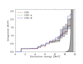
Figure 10: (Colour online) The observed integrated $B(\mathrm{GT})$ as a function of excitation energy for the decay of ³²Cl and comparison to shell-model calculations. For the experimental histogram (thick solid line with the shaded region representing its uncertainty bars), we have assumed zero Fermi strength in the 4695-keV state, zero Gamow-Teller strength in the IAS state, the range of Gamow-Teller strength given in the footnote of Table 4 for the 7190-keV state, and included the $\beta$-delayed particle emitting states from Ref. Honkanen et al. (1979). The hatched region indicates strength that may be missed in the experiment because the phase space for $\beta$ decay is too small resulting in $\beta$-delayed branches less than $0.0015\%$ which would not have been reported in Ref. Honkanen et al. (1979).

IV.2.2 Isospin-symmetry breaking in Fermi transitions

We switch our attention to the $\beta$ transition to the 7001-keV, $1^{+}_{2},T\!=\!1$ isobaric analogue state (IAS). This transition is a mix of Fermi and Gamow-Teller components; therefore from the partial half-life alone it is not possible to deduce the Gamow-Teller matrix element. Hence the gap in Table 4. However, the shell-model calculation for the Gamow-Teller matrix element predicts for the IAS state a very small value indeed. This is a fortunate happenstance: it gives us the opportunity to study this transition as if it were a pure Fermi type, compare it with the precisely measured pure Fermi transitions between $0^{+}$ states, and deduce the amount of isospin-symmetry breaking (ISB) in this transition. A fairly large ISB effect is anticipated because in ³²S the IAS state is only 189 keV away from the 7190-keV state; a state with the same spin but different isospin. Perturbation theory predicts that when two states of the same spin are close together in the spectrum, Coulomb and charge-dependent nuclear forces induce a degree of isospin-symmetry breaking that is inversely proportional to the square of the energy separation of the two states. For a separation of 189 keV, mixing at the several percent level can be anticipated.

The partial half-life for decay to the IAS state has been determined with $1\%$ accuracy, namely $t^{\mathrm{IAS}}=1.331(12)$ s. From this, the ISB correction $\delta_{C}$ can be determined to $15\%$ accuracy from the equation:

$$\begin{split}f_{\mathrm{exact}}\,t^{\mathrm{IAS}}&(1+\delta_{R}^{\prime})(1+\delta_{\mathrm{NS}}-\delta_{C})\\ &=\frac{K}{G_{V}^{2}(1+\Delta_{R}^{V})[B(\mathrm{F})+B(\mathrm{GT})]}\\ &=\frac{2\mathcal{F}t^{0^{+}\!\!\rightarrow 0^{+}}}{B(\mathrm{F})+B(\mathrm{GT})}.\end{split}$$ (11)

Here $K/(\hbar c)^{6}=2\pi^{3}\hbar\ln{2}/(m_{e}c^{2})^{5}$ is a constant and $G_{V}$ is the vector coupling constant characterizing the strength of the vector weak interaction. The quantity $K/G_{V}^{2}(1+\Delta_{R}^{V})$ is taken from the precision work on $0^{+}\!\!\rightarrow 0^{+}$ superallowed transitions and is expressed in terms of $\mathcal{F}t^{0^{+}\!\!\rightarrow 0^{+}}$ introduced in Eq. (7). The radiative correction has been split into three pieces: (a) a nucleus-independent term, $\Delta_{R}^{V}$, is included in $\mathcal{F}t^{0^{+}\!\!\rightarrow 0^{+}}\!$; (b) a trivially nucleus-dependent term, $\delta_{R}^{\prime}$, is calculated to be $1.421(32)\%$; and (c) a second nucleus-dependent term, $\delta_{\mathrm{NS}}$, is small but requires a nuclear-structure calculation to be evaluated. It is convenient to place $\delta_{\mathrm{NS}}$ and $\delta_{C}$ together as both are dependent on shell-model nuclear-structure calculations. Finally $B(\mathrm{F})$ is the square of the Fermi matrix element, $B(\mathrm{F})=|M_{0}|^{2}=2$ for $T\!=\!1$ transitions in the isospin-symmetry limit, and $B(\mathrm{GT})$ is the square of the Gamow-Teller matrix element, Eq. (7). For $B(\mathrm{GT})$, we take the three theoretical values from the shell-model calculation using USD, USD-A and USD-B effective interactions, average them and assign an uncertainty equal to half the spread between the largest and smallest calculated values: $B(\mathrm{GT})=0.002\pm 0.002$. On rearranging Eq. (11), we obtain

$$(\delta_{C}-\delta_{\mathrm{NS}})_{\mathrm{exp}} =1-\frac{2\langle\mathcal{F}t^{0^{+}\!\!\rightarrow 0^{+}}\rangle}{f_{\mathrm{exact}}\,t^{\mathrm{IAS}}(1+\delta_{R}^{\prime})\big{[}B(\mathrm{F})+B(\mathrm{GT})\big{]}}$$

$$=5.4(9)\%,$$ (12)

a substantial isospin symmetry breaking term, the largest yet determined in a superallowed Fermi transition.

In what follows we present a shell-model calculation of $\delta_{C}-\delta_{\mathrm{NS}}$ following the procedures developed by Towner and Hardy Towner and Hardy (2008). First, for the ISB correction $\delta_{C}$ defined in Eq. (1), the technique is to introduce Coulomb and other charge-dependent terms into the shell-model Hamiltonian. However, because the Coulomb force is long range, the shell-model space has to be very large indeed to include all the potential states with which the Coulomb interaction might connect. Currently this is not a practical proposition. To proceed, Towner and Hardy Towner and Hardy (2008) divide $\delta_{C}$ into two parts:

$$\delta_{C}=\delta_{C1}+\delta_{C2}.$$ (13)

For $\delta_{C1}$, we perform a shell-model calculation in the truncated $0\hbar\omega$ model space of the $s,d$-shell orbitals. Charge-dependent terms are added to the charge-independent Hamiltonians of USD, USD-A and USD-B. The strengths of these charge-dependent terms are adjusted to reproduce the $b=-5.4872(35)$ MeV and $c=0.1953(37)$ MeV Britz et al. (1998) coefficients of the isobaric multiplet mass equation (IMME) as applied to the $1^{+},T\!=\!1$ states in $A=32$, the triplet of states involved in the $\beta$-transition under study. As mentioned already, the bulk of the isospin mixing in the IAS occurs with the neighbouring $1^{+}_{3}$ state. This observation is used to constrain and refine the calculation. In the limit of two-state mixing, perturbation theory indicates that

$$\delta_{C1}\propto 1/(\Delta E)^{2},$$ (14)

where $\Delta E$ is the energy separation of the analogue and non-analogue $1^{+}$ states. Thus it is important that the shell-model Hamiltonian produce a good-quality spectrum of $1^{+}$ states. The shell model calculation has varying degrees of success in this regard. For the $1^{+}$ states in $A=32$, the separation between the IAS and the third $1^{+}_{3},T\!=\!0$ state is observed to be $188.9\pm 1.2$ keV.  The shell model calculates this separation to be 184 keV with USD, 248 keV with USD-A and 387 keV with USD-B interactions. These are quite respectable results given the inherent accuracy of a shell-model calculation for predicting energies. However, for a reliable $\delta_{C1}$ calculation, this spread in $\Delta E$ values is quite a problem. To cope with this, the Towner-Hardy recommended procedure is to scale the calculated $\delta_{C1}$ value by a factor of $(\Delta E)_{\mathrm{theo}}^{2}/(\Delta E)_{\mathrm{exp}}^{2}$, the ratio of the square of the energy separation of the $1^{+}$ states in the model calculation to that known experimentally. After this is done, the $\delta_{C1}$ values obtained in the three shell-model calculations are reasonably consistent: $\delta_{C1}=3.73\%$ for USD, $3.32\%$ for USD-A, and $4.19\%$ for USD-B. We average these three results and assign an uncertainty equal to half the spread between them to arrive at:

$$\delta_{C1}=3.75(45)\%.$$ (15)

For the calculation of $\delta_{C2}$ we need to consider mixing with states outside the $0\hbar\omega$ shell-model space. The principal mixing is with states that have one more radial node. Such mixing effectively changes the radial function of the proton involved in the $\beta$ decay relative to that of the neutron. The practical calculation, therefore, involves computing radial overlap integrals with modeled proton and neutron radial functions. Details of how this is done are given in Ref. Towner and Hardy (2008). The radial functions are taken to be eigenfunctions of a Saxon-Woods potential whose strength is adjusted so that the asymptotic form of the radial function has the correct dependence on the separation energy. The initial and final $A$-body states are expanded in a complete set of $(A\!-\!1)$-parent states. The separation energies are the energy differences between the $A$-body state and the $(A\!-\!1)$-body parent states. A shell-model calculation is required to give the spectrum of parent states and the spectroscopic amplitudes of the expansion. For the three USD interactions, we compute $\delta_{C2}=0.827\%$ for USD and $0.865\%$ for both USD-A and USD-B. Our adopted value is:

$$\delta_{C2}=0.85(3)\%.$$ (16)

The uncertainty, calculated in the same manner as described in Ref. Towner and Hardy (2008), represents the range of results for the USD interactions, the different methodologies considered in adjusting the strength of the Saxon-Woods potential, and the uncertainty in the Saxon-Woods radius parameter which was fitted to the experimental charge radius of ³²S.

Finally, we need an evaluation of the nuclear-structure-dependent piece of the radiative correction, $\delta_{\mathrm{NS}}$. Such a term arises because in a many-body system such as a nucleus, the electromagnetic interaction and the weak interaction that collectively induce a radiative correction do not have to interact with the same nucleon in the nucleus. When these interactions occur with different nucleons, the process is described by two-body operators. The evaluation of matrix elements of two-body operators depends in detail on the nuclear structure of the states involved. Such calculations were first made in 1992 Towner (1992); Barker et al. (1992) and updated two years later Towner (1994). We follow the latter reference and compute $\delta_{\mathrm{NS}}$ for each of the $s,d$-shell effective USD interactions. Essentially the same result was obtained in each case. We adopt the average value of

$$\delta_{\mathrm{NS}}=-0.15(2)\%.$$ (17)

The result is a very small correction, about 3 times smaller than the uncertainty in $\delta_{C}$.

Adding together Eqs. (15), (16) and (17), we obtain

$$\delta_{C}-\delta_{\mathrm{NS}}=4.8(5)\%,$$ (18)

which agrees with the experimental result of $5.4(9)\%$ of Eq. (12) within stated uncertainties. A comparison of this result with calculations for the $0^{+}\!\!\rightarrow 0^{+}$ cases is shown in Fig. 11. As one can clearly see, the correction in ³²Cl is about five times larger than the typical $<1\%$ values found for the $s,d$-shell nuclei in $0^{+}\!\!\rightarrow 0^{+}$ superallowed transitions. The TH model, which has already been shown Towner and Hardy (2010) to reproduce the nucleus-to-nucleus variation of ISB effects in superallowed zerotozero transitions required by the CVC hypothesis, is shown here to produce a much larger ISB effect as again verified by the current experiment.

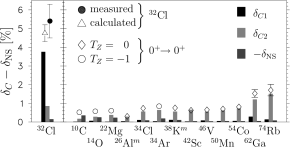
Figure 11: Our determination of the isospin-symmetry-breaking correction for ³²Cl (filled circle) and calculations for ³²Cl as well as other superallowed transitions (open points). The three components, $\delta_{C1}$, $\delta_{C2}$ and $\delta_{\mathrm{NS}}$, are shown separately. The measurement and prediction for ³²Cl, particularly the $\delta_{C1}$ component, is significantly larger than in any of the $0^{+}\!\!\rightarrow 0^{+}$ transitions.

Let us now briefly consider the isospin mixing in the non-analogue $1^{+}$ states at $7190$ and $4695$ keV, and deduce experimental values for the degree of mixing in the same way as just described for the IAS state. We assume the shell-model calculation for $B(\mathrm{GT})$ to be correct, assigning an uncertainty equal to half the spread between the different results obtained with the USD, USD-A and USD-B interactions. For the $7190$-keV state, the shell-model calculations yield $B(\mathrm{GT})=0.020(6)$, and for the $4695$-keV state $B(\mathrm{GT})=0.098(21)$. An experimental value for $B(\mathrm{F})+B(\mathrm{GT})$ is computed from a rearranged Eq. (12):

$$B_{\mathrm{exp}}(\mathrm{F})+B_{\mathrm{exp}}(\mathrm{GT})=\frac{2\mathcal{F}t^{0^{+}\!\!\rightarrow 0^{+}}}{f_{\mathrm{exact}}t(1+\delta_{R}^{\prime})},$$ (19)

where the nuclear-structure-dependent radiative correction, $\delta_{\mathrm{NS}}$, is ignored. Inserting the experimental values into the right-hand side of Eq. (19), we obtain

$$B_{\mathrm{exp}}(\mathrm{F})+B_{\mathrm{exp}}(\mathrm{GT}) =0.062\pm 0.005$$

$$B_{\mathrm{exp}}(\mathrm{F}) =0.042\pm 0.008$$ (20)

for the 7190-keV state, and

$$B_{\mathrm{exp}}(\mathrm{F})+B_{\mathrm{exp}}(\mathrm{GT}) =0.0790\pm 0.0012$$

$$B_{\mathrm{exp}}(\mathrm{F}) =-0.019\pm 0.021$$

$$\mathrm{or}\qquad B_{\mathrm{exp}}(\mathrm{F}) <0.014$$ (21)

for the 4695-keV state. In the limit of exact isospin symmetry the $B(\mathrm{F})$ values would be zero for these non-analogue transitions. So the non-zero value in Eq. (20) is a further indication that isospin-symmetry breaking is present. For non-analogue transitions, we define

$$B(\mathrm{F})=|M_{0}|^{2}\delta_{C1}^{n}(1-\delta_{C2})\simeq 2\delta_{C1}^{n}$$ (22)

where $\delta_{C1}^{n}$ is the isospin-symmetry breaking correction for the $n$^th $1^{+}$ state in ³²S computed in the $s,d$ shell-model space, and $\delta_{C2}$ the radial overlap correction representing Coulomb mixing beyond the $0\hbar\omega$ model space. In Eq. (22), we drop the $\delta_{C1}\delta_{C2}$ cross term as being negligible. From the experimental results in Eqs. (20) and (21), we determine $\delta_{C1,\,\mathrm{exp}}^{3}=2.1(4)\%$ for the 7190-keV state and $\delta_{C1,\,\mathrm{exp}}^{1}<0.7\%$ for the 4695-keV state. The theory calculation that produced the result for $\delta_{C1}$ in Eq. (15) also gives as a by-product values of $\delta_{C1}^{n}$ for the non-analogue transitions. For the 7190-keV and 4695-keV states, theory predicts $\delta_{C1}^{3}=3.2(3)\%$ and $\delta_{C1}^{1}=0.04(1)\%$ respectively. Evidently there is a small discrepancy between theory and experiment for the symmetry-breaking in the 7190-keV transition. On the theory side, if we accept the symmetry-breaking in the IAS state to be correct, then it is most likely to be correct in the 7190-keV state as well. This is because the situation is close to 2-state mixing, and the loss of Fermi strength to the IAS state is recovered in the 7190-keV state. On the experimental side, the result depends on the correctness of the Gamow-Teller strength calculated with USD wave functions. If the $B(\mathrm{GT})$ were over-estimated by the USD calculation, then theoretical and experimental values for the isospin symmetry mixing in the 7190-keV state could easily be reconciled.

V Conclusions

We have measured relative $\gamma$-ray intensities and deduced $\beta$-decay branches for the decay of ³²Cl. We have observed 3 new $\beta$ branches, 22 new $\gamma$ lines, placed limits on 2 other $\beta$ branches and 10 other $\gamma$ transitions, and have improved the precision on previously known yields and branches by about an order of magnitude.

In total, twelve $\beta$ branches have been measured in the decay of ³²Cl. Eleven of these are Gamow-Teller transitions and one is predominantly Fermi. For the Gamow-Teller transitions, the GT matrix element has been determined and compares favourably with shell-model calculations using USD effective interactions. These calculations also find the Gamow-Teller component in the IAS transition to be very small, indicating this transition is almost pure Fermi-like. Thus, this transition can be analyzed in an identical way to that used for the $0^{+}\!\!\rightarrow 0^{+}$ superallowed transitions. We extract a sizable isospin symmetry breaking correction for this transition, $\delta_{C}-\delta_{\mathrm{NS}}=5.4(9)\%$, which agrees well with a theoretical value of $4.8(5)\%$.

In addition, the improved precision in the relative $\gamma$-ray intensities can be used for a more precise determination of $\gamma$-ray efficiencies in the decay of ³²Ar Bhattacharya et al. (2008). The $\gamma$ intensity from the lowest $T\!=\!2$ state in ³²Cl is of interest for measuring isospin symmetry breaking in the $T\!=\!2$ superallowed decay of ³²Ar. Presently the $\gamma$-decay intensities from the decay of ³²Ar are limited by statistical precision, but the present work opens the possibility of determining its $\gamma$ branches to higher precision in future experiments.

VI Acknowledgments

We acknowledge the support staff of the Cyclotron Institute and the Center for Experimental Nuclear Physics and Astrophysics. The work of the Texas A&M authors is supported by the U.S. Department of Energy under Grant No. DE-FG02-93ER40773 and by the Robert A. Welch Foundation under Grant No. A-1397. The University of Washington authors were supported by the U.S. Department of Energy under Grant No. DE-FG02-97ER41020.

References

- Hardy and Towner (2009) J. C. Hardy and I. S. Towner, Phys. Rev. C 79, 055502 (2009).
- Hardy and Towner (2005a) J. C. Hardy and I. S. Towner, Phys. Rev. Lett. 94, 092502 (2005a).
- Hardy and Towner (2005b) J. C. Hardy and I. S. Towner, Phys. Rev. C 71, 055501 (2005b).
- Towner and Hardy (2008) I. S. Towner and J. C. Hardy, Phys. Rev. C 77, 025501 (2008).
- Auerbach (2009) N. Auerbach, Phys. Rev. C 79, 035502 (2009).
- Liang et al. (2009) H. Liang, N. V. Giai, and J. Meng, Phys. Rev. C 79, 064316 (2009).
- Satuła et al. (2011) W. Satuła, J. Dobaczewski, W. Nazarewicz, and M. Rafalski, Phys. Rev. Lett. 106, 132502 (2011).
- Miller and Schwenk (2008) G. A. Miller and A. Schwenk, Phys. Rev. C 78, 035501 (2008).
- Miller and Schwenk (2009) G. A. Miller and A. Schwenk, Phys. Rev. C 80, 064319 (2009).
- Hyland et al. (2006) B. Hyland et al., Phys. Rev. Lett. 97, 102501 (2006).
- Melconian et al. (2011) D. Melconian et al., Phys. Rev. Lett. 107, 182301 (2011).
- Triambak et al. (2006) S. Triambak et al., Phys. Rev. C 73, 054313 (2006).
- Ouellet and Singh (2011) C. Ouellet and B. Singh, Nucl. Data Sheets 112, 2199 (2011).
- Bhattacharya et al. (2008) M. Bhattacharya et al., Phys. Rev. C 77, 065503 (2008).
- Signoracci and Brown (2011) A. Signoracci and B. A. Brown, Phys. Rev. C 84, 031301 (2011).
- Wrede et al. (2010) C. Wrede et al., Phys. Rev. C 81, 055503 (2010).
- Tribble et al. (1991) R. Tribble, C. Gagliardi, and W. Liu, Nucl. Instrum. Methods Phys. Res. B 56-57, 956 (1991).
- Hardy et al. (2002) J. C. Hardy et al., Appl. Radiat. Isot. 56, 65 (2002).
- Helmer et al. (2003) R. G. Helmer et al., Nucl. Instrum. Methods Phys. Res. A 511, 360 (2003).
- Helmer et al. (2004) R. G. Helmer, N. Nica, J. C. Hardy, and V. E. Iacob, Appl. Radiat. Isot. 60, 173 (2004).
- Halbleib et al. (1992) J. A. Halbleib et al., ITS version 3.0: The Integrated TIGER Series of Coupled Electron/Photon Monte Carlo Transport Codes, Tech. Rep. SAND91-1634 (Sandia National Laboratory, 1992).
- Sempau et al. (1997) J. Sempau et al., Nucl. Instrum. Methods Phys. Res., Sect. B 132, 377 (1997).
- Kankainen et al. (2010) A. Kankainen et al., Phys. Rev. C 82, 052501 (2010).
- Audi et al. (2003) G. Audi, A. H. Wapstra, and C. Thibault, Nucl. Phys. A 729, 337 (2003).
- Shi et al. (2005) W. Shi, M. Redshaw, and E. G. Myers, Phys. Rev. A 72, 022510 (2005).
- Armini et al. (1968) A. J. Armini, J. W. Sunier, and J. R. Richardson, Phys. Rev. 165, 1194 (1968).
- Wilson et al. (1980) H. S. Wilson, R. W. Kavanagh, and F. M. Mann, Phys. Rev. C 22, 1696 (1980).
- Marquardt (1963) D. W. Marquardt, J. Soc. Industr. Appl. Math. 11, 431 (1963).
- Babilon et al. (2002) M. Babilon, T. Hartmann, P. Mohr, K. Vogt, S. Volz, and A. Zilges, Phys. Rev. C 65, 037303 (2002).
- Détraz et al. (1973) C. Détraz et al., Nucl. Phys. A 203, 414 (1973).
- Anderson et al. (1966) W. Anderson, L. Dillman, and J. Kraushaar, Nucl. Phys. 77, 401 (1966).
- Honkanen et al. (1979) J. Honkanen et al., Nuclear Physics A 330, 429 (1979).
- Hardy et al. (1977) J. C. Hardy et al., Phys. Lett. B 71, 307 (1977).
- Hardy and Towner (2002) J. C. Hardy and I. S. Towner, Phys. Rev. Lett. 88, 252501 (2002).
- Wildenthal (1984) B. H. Wildenthal, Prog. Part. Nucl. Phys. 11, 5 (1984).
- Brown and Richter (2006) B. A. Brown and W. A. Richter, Phys. Rev. C 74, 034315 (2006).
- Sirlin (1967) A. Sirlin, Phys. Rev. 164, 1767 (1967).
- Sirlin (1987) A. Sirlin, Phys. Rev. D 35, 3423 (1987).
- Jaus and Rasche (1987) W. Jaus and G. Rasche, Phys. Rev. D 35, 3420 (1987).
- Czarnecki et al. (2004) A. Czarnecki, W. J. Marciano, and A. Sirlin, Phys. Rev. D 70, 093006 (2004).
- Brown and Wildenthal (1985) B. A. Brown and B. H. Wildenthal, Atomic Data Nucl. Data Tables 33, 347 (1985).
- Brown and Wildenthal (1987) B. A. Brown and B. H. Wildenthal, Nucl. Phys. A 474, 290 (1987).
- Britz et al. (1998) J. Britz, A. Pape, and M. Antony, At. Data Nucl. Data Tables 69, 125 (1998).
- Towner (1992) I. S. Towner, Nucl. Phys. A 540, 478 (1992).
- Barker et al. (1992) F. C. Barker et al., Nucl. Phys. A 540, 501 (1992).
- Towner (1994) I. S. Towner, Phys. Lett. B 333, 13 (1994).
- Towner and Hardy (2010) I. S. Towner and J. C. Hardy, Phys. Rev. C 82, 065501 (2010).