Dynamical Mass Generation of Composite Dirac Fermions and Fractional Quantum Hall Effects near Charge Neutrality in Graphene

Abstract

We develop a composite Dirac fermion theory for the fractional quantum Hall effects (QHE) near charge neutrality in graphene. We show that the interactions between the composite Dirac fermions lead to a dynamical mass generation through exciton condensation. The four-fold spin-valley degeneracy is fully lifted due to the mass generation and the exchange effects such that the odd-denominator fractional QHE observed in the vicinity of charge neutrality can be understood in terms of the integer QHE of the composite Dirac fermions. At the filling factor $\nu=1/2$, we show that the massive composite Dirac fermion liquid is unstable against chiral $p$-wave pairing for weak Coulomb interactions and the ground state is a paired nonabelian quantum Hall state described by the Moore-Read Pfaffian in the long wavelength limit.

I Introduction

Since the discovery of graphene graphene , a rich set of integer Novoselov ; YZhang1 ; YZhang2 ; Jiang and fractional Du ; Bolotin ; Ghahari ; Dean quantum Hall effects (QHE) has been explored experimentally under the new setting of two-dimensional lattice electrons with a relativistic energy-momentum dispersion at low energy. Currently, the $\nu=1/3$ state has been convincingly observedDu ; Bolotin ; Ghahari ; Dean ; Feldman1 ; Feldman2 . Remarkably, initial evidence for the emergence of a $\nu=1/2$ fractional quantum Hall state has been reported Ghahari , raising the hope for realizing nonabelian statistics in suspended graphene.

For graphene, it is known that there is a spin-valley SU(4) symmetry. This restricts the filling factors $\nu$ of the integer QHE of the Dirac fermions to $\pm 2,\pm 6,\pm 10,\cdots$, provided that the SU(4) symmetry is unbroken. The observation of the $\nu=\pm 1$ integer Hall plateaus YZhang1 indicates that the SU(4) symmetry is broken. Dynamical mass generation, which lifts the spin-valley degeneracy of the zeroth Dirac Landau level ($\zeta LL$) mc , as well as quantum Hall ferromagnetism MacDonald ; Alicea ; KYang have been proposed for its explanation. Despite recent theoretical efforts on the fractional QHE (FQHE) in graphene KYang ; Apalkov ; Toke1 ; Goerbig ; Khveshchenko ; Papic , it remains uncertain whether the observed $\nu=1/3$ state implies SU(4) symmetry breaking and is therefore a single-component Laughlin state, or a multi-component Halperin state with spin-valley degeneracy Papic . Moreover, although states at even-denominator filling factors have been investigated numerically Toke2 ; Wojs by exact-diagonalization, the effect of Landau level mixing, which may be relevant for the stabilization of the Moore-Read Pfaffian state BN ; WTJ ; Rezayi ; Sodemann ; Peterson ; Simon , was neglected when the Hilbert space is projected and restricted to that of a specific Landau level.

In this paper, we propose a mechanism of dynamical mass generation by exciton condensation and exchange-driven polarization to qualitatively describe both the abelian and the nonabelian FQHE in graphene. To this end, we extend the composite fermion Chern-Simons (CS) theory HLR ; Jain to the case of Dirac particles attached to an even number of flux quanta through the CS gauge field, which can be implemented by a unitary transformation. We will refer to this transformation as the CS transformation.

The CS approach is more suitable for studying the fractional quantum Hall regime where Landau level mixing is significant, since it does not restrict the quantum states to the $\zeta LL$. The importance of Landau level mixing in graphene can be seen from the fact that, contrary to semiconductor heterostructures where the dispersion is non-relativistic, the Coulomb interaction energy and Landau level spacing for Dirac fermions both scale with $\sqrt{B}$, where $B$ is the strength of the magnetic field. Specifically, the ratio of the interaction energy and energy spacing between the zeroth and first Landau levels is given by $\alpha_{g}/\sqrt{2}$ where $\alpha_{g}=e^{2}/4\pi\epsilon\hbar v_{F}$ is the fine structure constant for graphene. For free standing graphene, the bare value of the fine structure constant is $\alpha_{g}\approx 2.2$ (see e.g., Ref. Drut ). Therefore, the two energy scales are of the same order; the system should be in the strong coupling regime mc where Landau level spacing is a relevant energy scale.

A crucial step in our theory is to work with the proper particle density via a particle-hole transformation such that the vacuum state of the relativistic composite Dirac fermions (CDF) is defined by the charge neutral state with all negative energy states filled. The CDF theory introduced in this paper are rather general, involving only relations between the CDF particle density and its filling fraction $\widetilde{\nu}$. As we will show, the latter corresponds to a unique filling fraction $\nu$ of the original electrons once the ground state is determined.

At the filling fractions $\widetilde{\nu}=\pm 1/\widetilde{\phi}$ with $\widetilde{\phi}$ an even integer, we will show, by variational calculations of the ground state energy, that it is energetically favorable for the CDF to develop an exciton condensate. The latter supports single quasiparticle excitations with a CDF mass gap at low density above the condensate. It turns out that the possible CS transformations can be grouped into three types depending on whether the SU(4) symmetry is broken and how it is broken. If the exciton mass gaps have the same sign for all SU(4) components, the SU(4) symmetry is preserved. This kind of CDF systems have a non-zero Chern number $\pm 2$, implying that the exciton condensate is an anomalous Hall liquid. In terms of the Bloch electrons in graphene, this corresponds to a total filling factor $\nu=\pm(2-\widetilde{\nu})$. However, when the exciton mass gaps for different SU(4) components are of different signs, the SU(4) symmetry is broken and the spin-valley degeneracy is lifted. There are two ways to break the symmetry since we have two inequivalent ways to partition the four spin-valley components into two groups. In the first case, one of the components has a different sign from the remaining three; in the second case, the four components are divided evenly into two groups. The former has Chern number $\pm 1$ and describes electron states at $\nu=\pm(1-\widetilde{\nu})$. The latter is topologically trivial with net Chern number zero. It therefore describes the electron states at filling fractions $\nu=\pm\widetilde{\nu}$. In this case, the exchange term in the statistical interaction further breaks the remaining symmetry so that the ground state is fully spin-valley polarized.

Thus, in the present theory, the dynamical SU(4) symmetry-breaking mass generation offers a route to the observed FQHE states in graphene near charge neutrality Du ; Bolotin ; Ghahari ; Dean . We show that the quasiparticles above the exciton condensate have a pairing instability in the chiral $p$-wave channel, leading to an even denominator paired quantum Hall state described by the nonabelian Moore-Read Pffafian MR ; RG in the long wavelength limit. On the other hand, at odd-denominator filling fractions such as $\nu=1/3$, the quasiparticles above the exciton condensate occupy fully filled Landau levels of the residual magnetic field Jain , giving rise to a single-component Laughlin state for the electrons in graphene.

The key ingredient of the present theoretical framework is the dynamical mass generation of massless Dirac fermions, which enables us to approach the FQHEs near filling factors $\nu=0,\pm 1,\pm 2$ in a unified way. This is an exciting example of the interplay between condensed matter and high energy physics; as the mechanism was introduced by Nambu and Jona-Lasinio Nambu inspired by the BCS theory of superconductivity. It was used recently to explain Landau level splitting mc in graphene. Here we extend this mechanism to the FQHE of lattice electrons in graphene, thus provide another physical realization of dynamical mass generation in a condensed matter system. We note that such an excitonic mass generation intrinsically involves Landau level mixing since it requires the formation of particle-hole pairs consisting of states from different Landau levels.

This paper is structured as follows. In Section II, we formulate the composite Dirac fermion theory by introducing a unitary transformation that implements the flux attachment. We then derive the statistical interaction mediated by the CS gauge field, focusing on the even denominator filling factors where the external magnetic field is canceled by the flux of the CS field. The effects of the statistical interaction is then investigated. In Section III, we show that an immediate consequence of the statistical interaction is the exciton condensation which opens up mass gaps for the four components of the CDFs. The normal state is obtained by doping the exciton insulating state according to the filling factors of the fractional quantum Hall states. In Section IV, we study the pairing instability induced by the statistical interaction. We show that the leading instability is in the complex $p$-wave channel which provides a realization of the nonabelian Moore-Read state in graphene.

II Theory of composite Dirac fermions

We start with graphene electrons in the continuum limit under a perpendicular external magnetic field $\mathbf{B}=-B\hat{\mathbf{z}}$. The effective Hamiltonian can be written down in terms of the four-component fermion operator $\psi_{s}(\mathbf{x})$ for the two-sublattice and two-valley degrees of freedom,

$$H=-i\hbar v_{F}\int\,\text{d}^{2}x\psi_{s}^{\dagger}\alpha_{i}(\partial_{i}+ieA_{i}/\hbar)\psi_{s},$$ (1)

where $v_{F}$ is the Fermi velocity and $A_{i}(\mathbf{x})$ is the vector potential: $\nabla\times\mathbf{A}=\mathbf{B}$. The summations over repeated spin index $s$ and the spatial index $i=1,2$ are implied. The $4\times 4$ matrix $\alpha_{i}=\gamma^{0}\gamma^{i}$, with the $\gamma$ matrices given by $\gamma^{0}=I\otimes\tau_{1}$, $\gamma^{i}=-i\sigma_{i}\otimes\tau_{2}$, where $\sigma_{i}$ and $\tau_{i}$ are the $2\times 2$ Pauli matrices acting in the sublattice and valley subspaces, respectively. To make the SU(4) symmetry explicit, it is instructive to separate out the valley degrees of freedom and rewrite the Hamiltonian as

$$H =-i\hbar v_{F}\int\,\text{d}^{2}x\psi_{Rs}^{\dagger}(\mathbf{x})\sigma_{i}\left(\partial_{i}+i\frac{e}{\hbar}A_{i}\right)\psi_{Rs}(\mathbf{x})$$

$$+i\hbar v_{F}\int\,\text{d}^{2}x\psi_{Ls}^{\dagger}(\mathbf{x})\sigma_{i}\left(\partial_{i}+i\frac{e}{\hbar}A_{i}\right)\psi_{Ls}(\mathbf{x}).$$ (2)

Here $\psi_{\tau s}(\mathbf{x})$ is a two-component fermion spinor field for spin $s=\uparrow,\downarrow$ and valley $\tau=R,L$. For convenience, we denote $\psi_{\tau s}=\psi_{\alpha}$ with $\alpha=\{1,2,3,4\}=\{(\downarrow,R),(\downarrow,L),(\uparrow,R),(\uparrow,L)\}$.

The CDF field $\Psi_{\alpha}$ can be introduced by a unitary transformation

$$\left(\begin{array}[]{c}\psi_{1}\\ \psi_{2}\\ \psi_{3}\\ \psi_{4}\end{array}\right)=\begin{pmatrix}e^{i\mathcal{I}_{1}}&&0&&0&&0\\ 0&&e^{i\mathcal{I}_{2}}&&0&&0\\ 0&&0&&e^{i\mathcal{I}_{3}}&&0\\ 0&&0&&0&&e^{i\mathcal{I}_{4}}\\ \end{pmatrix}\left(\begin{array}[]{c}\Psi_{1}\\ \Psi_{2}\\ \Psi_{3}\\ \Psi_{4}\end{array}\right),$$ (11)

with

$${\cal I}_{\alpha}(\mathbf{x})=\sum_{\beta}\int\,\text{d}^{2}x^{\prime}\mathcal{K}_{\alpha\beta}\rho_{\beta}(\mathbf{x}^{\prime})\arg(\mathbf{x}-\mathbf{x}^{\prime}),$$ (12)

where $\alpha,\beta=1,2,3,4$ and $\rho_{\alpha}$ is the particle density operator in the spin-valley sector $\alpha$. Note that due to the presence of multiple components, a $\mathcal{K}$-matrix must be introduced in the unitary transformation Wen . Its physical meaning is explained below. The form of the $\mathcal{K}$-matrix can be specified by physical considerations. In order for the CDF field $\Psi_{\alpha}(\mathbf{x})$ to be fermionic, $\mathcal{K}$ must be symmetric and its diagonal elements must be even Rajaraman .

The transformed Hamiltonian, i.e. the Hamiltonian of the CDFs is given by

$$H=(-1)^{\alpha}i\hbar v_{F}\int\,\text{d}^{2}x\Psi_{\alpha}^{\dagger}\sigma_{i}\left[\partial_{i}+i{e\over\hbar}(A_{i}+a^{\alpha}_{i})\right]\Psi_{\alpha},$$ (13)

with the CS gauge field $\mathbf{a}^{\alpha}=(a_{1}^{\alpha},a_{2}^{\alpha})$:

$$a^{\alpha}_{1}(\mathbf{x}) =\frac{\hbar}{e}\sum_{\beta}\mathcal{K}_{\alpha\beta}\int\,\text{d}^{2}x^{\prime}\frac{-(x_{2}-x^{\prime}_{2})}{|\mathbf{x}-\mathbf{x}^{\prime}|^{2}}\rho_{\beta}(\mathbf{x}^{\prime}),$$

$$a^{\alpha}_{2}(\mathbf{x}) =\frac{\hbar}{e}\sum_{\beta}\mathcal{K}_{\alpha\beta}\int\,\text{d}^{2}x^{\prime}\frac{x_{1}-x^{\prime}_{1}}{|\mathbf{x}-\mathbf{x}^{\prime}|^{2}}\rho_{\beta}(\mathbf{x}^{\prime}).$$ (14)

It is straightforward to verify that $\mathbf{a}^{\alpha}$ satisfies

$$\nabla\times\mathbf{a}^{\alpha}(\mathbf{x})=\hat{\mathbf{z}}\sum_{\beta}\mathcal{K}_{\alpha\beta}\rho_{\beta}(\mathbf{x})h/e.$$ (15)

Physically, Eq. (15) describes how the CS gauge field coupled to the CDFs with the spin-valley index $\alpha$ is generated by the flux quanta attached to other CDFs in the same or different spin-valley sectors. The number of flux quantum is specified by the matrix elements of $\mathcal{K}$. We note that $\rho_{\alpha}$ can be either positive or negative due to the particle-hole symmetry of the Dirac spectrum and our choice of vacuum associated with the charge neutral point. As a result, the matrix elements of $\mathcal{K}$ can be positive or negative. In particular, if $\mathcal{K}$ describes a state with filling factor $\widetilde{\nu}$, $-\mathcal{K}$ describes a state with filling factor $-\widetilde{\nu}$. The condition for the CDFs to experience a vanishing net magnetic field on average requires

$$\sum_{\beta}\mathcal{K}_{\alpha\beta}\braket{\rho_{\beta}}=eB/h$$ (16)

for all the values of $\alpha$. For a given filling fraction $\widetilde{\nu}=\sum_{\alpha}\braket{\rho_{\alpha}}h/eB=\pm 1/\widetilde{\phi}$, there are three types of physical solutions:

$$\mathcal{K}^{1} =\mathrm{sgn}(\widetilde{\nu})\begin{pmatrix}\widetilde{\phi}&\widetilde{\phi}&\widetilde{\phi}&\widetilde{\phi}\\ \widetilde{\phi}&\widetilde{\phi}&\widetilde{\phi}&\widetilde{\phi}\\ \widetilde{\phi}&\widetilde{\phi}&-\widetilde{\phi}&-\widetilde{\phi}\\ \widetilde{\phi}&\widetilde{\phi}&-\widetilde{\phi}&-\widetilde{\phi}\end{pmatrix},$$

$$\mathcal{K}^{2} =\mathrm{sgn}(\widetilde{\nu})\begin{pmatrix}\widetilde{\phi}&\widetilde{\phi}&\widetilde{\phi}&\widetilde{\phi}\\ \widetilde{\phi}&\widetilde{\phi}&\widetilde{\phi}&\widetilde{\phi}\\ \widetilde{\phi}&\widetilde{\phi}&\widetilde{\phi}&\widetilde{\phi}\\ \widetilde{\phi}&\widetilde{\phi}&\widetilde{\phi}&-\widetilde{\phi}\end{pmatrix},$$

$$\mathcal{K}^{3} =\mathrm{sgn}(\widetilde{\nu})\begin{pmatrix}\widetilde{\phi}&\widetilde{\phi}&\widetilde{\phi}&\widetilde{\phi}\\ \widetilde{\phi}&\widetilde{\phi}&\widetilde{\phi}&\widetilde{\phi}\\ \widetilde{\phi}&\widetilde{\phi}&\widetilde{\phi}&\widetilde{\phi}\\ \widetilde{\phi}&\widetilde{\phi}&\widetilde{\phi}&\widetilde{\phi}\end{pmatrix}.$$ (17)

An obvious distinction among the $\mathcal{K}$ matrices is that $\mathcal{K}^{1}$ and $\mathcal{K}^{2}$ break the $\mathrm{SU}(4)$ symmetry while $\mathcal{K}^{3}$ preserves the full symmetry. This can be seen from the CS transformation (11). If all four spin-valley components rotate in the same way, $\mathrm{SU}(4)$ symmetry is preserved. This requires the operator $\mathcal{I}_{\alpha}(\mathbf{x})$ to be identical for the four components. This condition, together with the general requirements for the $\mathcal{K}$-matrix mentioned above, uniquely determines $\mathcal{K}^{3}$. On the other hand, the CS transformation associated with $\mathcal{K}^{1}$ rotates the two spin components differently, thus leads to a broken $\mathrm{SU}(2)$ spin symmetry. Furthermore, the solution of Eq. (16) for $\mathcal{K}^{1}$ requires $\braket{\rho_{\downarrow}}=eB/h\widetilde{\phi}$, $\braket{\rho_{\uparrow}}=0$ for $\widetilde{\nu}=1/\widetilde{\phi}$, where $\rho_{\downarrow}=\rho_{1}+\rho_{2}$ and $\rho_{\uparrow}=\rho_{3}+\rho_{4}$. Thus $\mathcal{K}^{1}$ describes a state in which spin is fully polarized. Equivalently, one can interchange the spin and valley to break the valley symmetry this way, resulting in a $\mathcal{K}$-matrix of similar structure as $\mathcal{K}^{1}$. Interestingly, the $\mathrm{SU}(4)$ symmetry can be broken in another way, i.e., by keeping any three of the spin-valley components degenerate while rotating the remaining component in a different way. This is achieved by the $\mathcal{K}^{2}$. Similar to $\mathcal{K}^{1}$, this matrix implies a constraint $\braket{\rho_{4}}=0$ when $\widetilde{\nu}=1/\widetilde{\phi}$. We will show that the CDFs have different topological properties when they are in the states specified by these three characteristic $\mathrm{K}$-matrices. Note that, due to the particle-hole symmetry, the $\mathcal{K}$-matrices for positive (particle) and negative (hole) filling factors have opposite signs. As a result, some of the $\mathcal{K}$-matrices have negative eigenvalues. This should be contrasted to the case of non-relativistic multi-component electron systems where the $\mathcal{K}$-matrices with negative eigenvalues result in wavefunctions that are not normalizable Beugeling , as a consequence of the quadratic energy-momentum dispersion.

The expressions for $\mathcal{K}^{1}$ and $\mathcal{K}^{3}$ can be further simplified by noting that the two valleys for a given spin projection are degenerate in these states. As a result, the $\mathcal{K}$-matrices in this case effectively reduces to $2\times 2$ matrices. Let $\Psi_{\downarrow}=(\Psi_{1},\Psi_{2})^{T}$ and $\Psi_{\uparrow}=(\Psi_{3},\Psi_{4})^{T}$, the CS transformation can be expressed as

$$\left(\begin{array}[]{c}\psi_{\downarrow}(\mathbf{x})\\ \psi_{\uparrow}(\mathbf{x})\end{array}\right)=\begin{pmatrix}e^{i\mathcal{I}_{\downarrow}(\mathbf{x})}&&0\\ 0&&e^{i\mathcal{I}_{\uparrow}(\mathbf{x})}\end{pmatrix}\left(\begin{array}[]{c}\Psi_{\downarrow}(\mathbf{x})\\ \Psi_{\uparrow}(\mathbf{x})\end{array}\right),$$ (22)

with

$${\cal I}_{s}(\mathbf{x})=\sum_{s^{\prime}}\int\,\text{d}^{2}x^{\prime}\mathcal{K}_{ss^{\prime}}\rho_{s^{\prime}}(\mathbf{x}^{\prime})\arg(\mathbf{x}-\mathbf{x}^{\prime}),$$ (23)

and

$$\mathcal{K}^{1}=\begin{pmatrix}\widetilde{\phi}&\mathrm{sgn}(\widetilde{\nu})\widetilde{\phi}\\ \mathrm{sgn}(\widetilde{\nu})\widetilde{\phi}&-\widetilde{\phi}\end{pmatrix},\quad\mathcal{K}^{3}=\mathrm{sgn}(\widetilde{\nu})\begin{pmatrix}\widetilde{\phi}&\widetilde{\phi}\\ \widetilde{\phi}&\widetilde{\phi}\end{pmatrix}.$$ (24)

Under the transformation,

$$H=-i\hbar v_{F}\int\,\text{d}^{2}x\Psi_{s}^{\dagger}\alpha_{i}(\partial_{i}+ie(A_{i}+a^{s}_{i})/\hbar)\Psi_{s}.$$ (25)

To keep the presentation simple, we will focus on $\mathcal{K}^{1}$ and $\mathcal{K}^{3}$, and comment on $\mathcal{K}^{2}$ when appropriate.

The Hamiltonian $H$ in Eq. (25) can be separated into two parts

$$H=H_{0}+V_{\mathrm{st}},$$ (26)

where $H_{0}$ is the Hamiltonian for free massless Dirac particles and $V_{\mathrm{st}}$ describes the CDF interactions mediated by the CS gauge field. It can be obtained from the $A_{i}+a^{s}_{i}$ terms by using the explicit expressions for $a^{s}_{i}$ in Eq. (II) and writing the vector potential $A_{i}$ in terms of the average density $\braket{\rho_{s}}$. The final result is an interaction of the form:

$$V_{\mathrm{st}}= \sum_{s}-i\hbar v_{F}\int\,\text{d}^{2}x\,\text{d}^{2}x^{\prime}\left(\Psi^{\dagger}_{Rs}(\mathbf{x})\mathcal{M}_{s}(\mathbf{x},\mathbf{x}^{\prime})\Psi_{Rs}(\mathbf{x})\right.$$

$$\left.-\Psi^{\dagger}_{Ls}(\mathbf{x})\mathcal{M}_{s}(\mathbf{x},\mathbf{x}^{\prime})\Psi_{Ls}(\mathbf{x})\right),$$ (27)

where,

$$\mathcal{M}_{s}(\mathbf{x},\mathbf{x}^{\prime})=\sum_{s^{\prime}}\mathcal{K}_{ss^{\prime}}\delta\rho_{s^{\prime}}(\mathbf{x}^{\prime})\begin{pmatrix}0&1/(z-z^{\prime})\\ -1/(\bar{z}-\bar{z}^{\prime})&0\end{pmatrix},$$

with the bilinear fermion operator $\delta\rho_{s}=\rho_{s}-\langle\rho_{s}\rangle$, and the holomorphic coordinates $z=x+iy$, $\bar{z}=x-iy$. We will refer to $V_{\mathrm{st}}$, which is essentially a CDF current-density interaction, as the statistical interaction.

Since the CDF experiences zero net magnetic field, its field operator can be conveniently expanded in the helicity basis as

$$\Psi_{Rs}(\mathbf{x}) =\frac{1}{\sqrt{2\mathcal{V}}}\sum_{\mathbf{k}}e^{i\mathbf{k}\cdot\mathbf{x}}\left[\begin{pmatrix}e^{-i\theta_{\mathbf{k}}}\\ 1\end{pmatrix}A_{s\mathbf{k}}+\begin{pmatrix}e^{-i\theta_{\mathbf{k}}}\\ -1\end{pmatrix}B^{\dagger}_{s\mathbf{k}}\right],$$

$$\Psi_{Ls}(\mathbf{x}) =\frac{1}{\sqrt{2\mathcal{V}}}\sum_{\mathbf{k}}e^{i\mathbf{k}\cdot\mathbf{x}}\left[\begin{pmatrix}e^{-i\theta_{\mathbf{k}}}\\ -1\end{pmatrix}C_{s\mathbf{k}}+\begin{pmatrix}e^{-i\theta_{\mathbf{k}}}\\ 1\end{pmatrix}D^{\dagger}_{s\mathbf{k}}\right],$$

where $\theta_{\mathbf{k}}=\arctan k_{y}/k_{x}$. Note that, in the operator expansion, we have performed a particle-hole transformation such that removing a particle in a negative energy state is redefined as creating a hole with positive energy. Specifically, $B^{\dagger}_{s\mathbf{k}}$ and $D^{\dagger}_{s\mathbf{k}}$ in the above expressions are the hole creation operators for the $R$- and $L$-valleys respectively. In the helicity basis, the kinetic energy part of the Hamiltonian becomes

$$H_{0}=\sum_{s\mathbf{k}}\hbar v_{F}k(A^{\dagger}_{s\mathbf{k}}A_{s\mathbf{k}}+B^{\dagger}_{s\mathbf{k}}B_{s\mathbf{k}}+C^{\dagger}_{s\mathbf{k}}C_{s\mathbf{k}}+D^{\dagger}_{s\mathbf{k}}D_{s\mathbf{k}}).$$ (28)

III Exciton condensation and normal states

The statistical interaction derived in the previous section has important physical consequences on the nature of the ground states for the CDFs. We now show that it drives the formation of an exciton condensate of the CDFs. The normal state is obtained by populating quasi-particles on top of the exciton condensate. In other words, the normal state of the CDFs corresponds to doping an excitonic insulator. We shall use the variational approach and construct a variational wavefunction for the normal. First, at charge neutrality, the exciton vacuum can be written as follows,

$$\ket{0}= \prod_{s}\prod_{\mathbf{k}}\left(\cos\varphi_{Rs\mathbf{k}}-\sin\varphi_{Rs\mathbf{k}}A^{\dagger}_{s\mathbf{k}}B^{\dagger}_{s\mathbf{k}}\right)$$

$$\times\left(\cos\varphi_{Ls\mathbf{k}}-\sin\varphi_{Ls\mathbf{k}}C^{\dagger}_{s\mathbf{k}}D^{\dagger}_{s\mathbf{k}}\right)\ket{\mathrm{vac}},$$ (29)

where $\varphi_{R,L}$ are variational parameters and $\ket{\mathrm{vac}}$ describes the state where the valence CDF bands are filled and the conduction bands empty. The quasiparticle operators associated with the exciton condensate $|0\rangle$ can be obtained through a Bogoliubov transformation and are given by,

$$a^{\dagger}_{s\mathbf{k}} =\cos\varphi_{Rs\mathbf{k}}A^{\dagger}_{s\mathbf{k}}+\sin\varphi_{Rs\mathbf{k}}B_{s\mathbf{k}},$$

$$b_{s\mathbf{k}} =-\sin\varphi_{Rs\mathbf{k}}A^{\dagger}_{s\mathbf{k}}+\cos\varphi_{Rs\mathbf{k}}B_{s\mathbf{k}},$$ (30)

for the $R$-valley and similarly in terms of $c^{\dagger}_{s\mathbf{k}}$ and $d_{s\mathbf{k}}$ for the $L$-valley (not shown). It is straightforward to verify that $\ket{0}$ contains no quasiparticles, i.e. $a_{s\mathbf{k}}\ket{0}=b_{s\mathbf{k}}\ket{0}=0$.

The normal state with a nonzero particle density can be constructed by creating quasiparticles on top of the exciton vacuum $\ket{0}$. A generic normal state with a positive filling factor can be written as $\ket{N}=\prod_{s}\prod_{k\leq k^{Rs}_{F}}a^{\dagger}_{s\mathbf{k}}\prod_{k\leq k^{Ls}_{F}}c^{\dagger}_{s\mathbf{k}}\ket{0}$ where $k_{F}^{Rs}$ and $k_{F}^{Ls}$ are the Fermi wave vectors associated with the two valleys with spin $s$. At the filling factor $\widetilde{\nu}$, we have

$$\sum_{s,k\leq k^{Rs}_{F}}\braket{N}{a^{\dagger}_{s\mathbf{k}}a_{s\mathbf{k}}}{N}+\sum_{s,k\leq k^{Ls}_{F}}\braket{N}{c^{\dagger}_{s\mathbf{k}}c_{s\mathbf{k}}}{N}=\widetilde{\nu}eB/h.$$ (31)

Hereafter, the wave vector will be measured in unit of $k_{F}=1/l_{B}\widetilde{\phi}^{1/2}$, which corresponds to the spin-polarized CDF Fermi vector, and the energy in unit of $\hbar v_{F}k_{F}$. We will show that the variational energy is indeed minimized at nonzero $\varphi_{R,L}$ in favor of an exciton condensate.

It is useful to note that the exciton condensation energy from the statistical interaction is linear in the exciton mass. This is due to the fact that $V_{\mathrm{st}}$ is a current-density interaction and can be expressed as,

$$V_{\mathrm{st}}=i\sum_{s,s^{\prime}}\mathcal{K}_{ss^{\prime}}$$

$$\times\int\,\text{d}^{2}x\,\text{d}^{2}x^{\prime}\bar{\Psi}_{s}(\mathbf{x})\gamma^{3}\gamma^{5}\Psi_{s^{\prime}}(\mathbf{x}^{\prime})\frac{(\mathbf{x}-\mathbf{x}^{\prime})\cdot\mathbf{J}_{s^{\prime}s}(\mathbf{x}^{\prime},\mathbf{x})}{|\mathbf{x}-\mathbf{x}^{\prime}|^{2}},$$ (32)

where $J_{i,s^{\prime}s}(\mathbf{x}^{\prime},\mathbf{x})=\bar{\Psi}_{s^{\prime}}(\mathbf{x}^{\prime})\gamma^{i}\Psi_{s}(\mathbf{x})$. The internal energy coming from the statistical interaction $\braket{V_{\mathrm{st}}}$ is a linear function of the exciton order parameter $\braket{\bar{\Psi}_{s}(\mathbf{x})\gamma^{3}\gamma^{5}\Psi_{s}(\mathbf{x}^{\prime})}$. As a result, the mass has the same sign as that of the corresponding matrix elements in $\mathcal{K}$ in order to lower the energy. To gain further insight, one can isolate the interaction $V_{\mathrm{st}}$ in the exchange channel (e.g., for the $R$-valley)

$$F_{\mathrm{st}}= -\frac{\pi}{\mathcal{V}}\sum_{s,\mathbf{k},\mathbf{p}}\mathcal{K}_{ss}\frac{\sin 2\varphi_{Rs\mathbf{k}_{<}}\cos 2\varphi_{Rs\mathbf{k}_{>}}}{k_{>}}a^{\dagger}_{s\mathbf{k}}a_{s\mathbf{k}}a^{\dagger}_{s\mathbf{p}}a_{s\mathbf{p}}$$ (33)

where $\mathbf{k}_{>}$ ($\mathbf{k}_{<}$) is the bigger (smaller) of $\mathbf{k}$ and $\mathbf{p}$. To lower the energy, i.e. to have a negative $F_{\mathrm{st}}$, $\mathcal{K}_{ss}$ and $\varphi_{Rs\mathbf{k}}$ must have the same sign and a positive $\varphi$ implies a positive mass. The diagonal elements of $\mathcal{K}^{1}$ have opposite signs, leading to opposite masses for the spin-down and spin-up CDF bands. In contrast, the diagonal elements of $\mathcal{K}^{3}$ have the same sign and thus produce mass gaps that are all positive. For zeroth Landau level, the energy is given by the mass, e.g., if the mass is negative, the energy of the zeroth Landau level will be negative. Thus for different $\mathcal{K}$-matrices, the $\zeta LL$s have different configurations as illustrated in Fig. 1. More importantly, the transport property of Dirac fermions depends on the sign of the mass since the direction of the Hall current is different for different masses when the chemical potential lies in the mass gap. This property is characterized by a topological number called the Chern number TIReview .

The exciton condensation is thus essential for classifying the different states described by the three types of the ${\cal K}$ matrices. The difference lies in the topology characterized by the Chern number of the CDF bands, which is determined by the sign of the mass. Indeed, from the sign of the mass gap, one can read out the Chern number of different states described by the ${\cal K}$ matrices. For $\mathcal{K}^{1}$, the SU(4) symmetry breaking leads to different signs in the mass gaps. The occupied bands has a zero total Chern number and so the total filling factor is given by $\nu=\widetilde{\nu}=\pm 1/\widetilde{\phi}$. For the SU(4) symmetric case described by ${\cal K}^{3}$, the identical mass gaps contribute to a non-vanishing total Chern number $\pm 2$, resulting in a quantum anomalous Hall effect (QAHE) for the CDFs. Remarkably, this QAHE at $\widetilde{\nu}$ implies that the total filling factor $\nu=\pm(2-1/\widetilde{\phi})$ for the electrons, where the integer contribution to $\sigma_{xy}$ comes from the QAHE of the exciton condensate. Similarly, $\mathcal{K}^{2}$ describes states at filling factor $\nu=\pm(1-1/\widetilde{\phi})$ since it leads to CDF bands with Chern number $\pm 1$. In the rest of the paper, our focus will be on the FQHE in the vicinity of charge neutrality observed in recent experiments Du ; Bolotin ; Ghahari ; Dean .

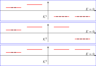
Figure 1: (color online) Schematic plots of the zeroth Landau levels for different $\mathcal{K}$-matrices. The lines with four dots depict completely filled Landau levels, and lines with two dots means partially filled Landau levels. The difference between the $\mathcal{K}$ matrices is reflected in the signs of the exciton mass gaps, and thus the relative positions of the zeroth Landau levels with respect to zero energy. $\mathcal{K}^{1}$ leads to opposite masses for the two spin projections and therefore describes the $\nu=1/\widetilde{\phi}$ state (top panel). $\mathcal{K}^{2}$ has one component with a different sign, corresponding to the filling factor $\nu=-1+1/\widetilde{\phi}$ (middle panel). $\mathcal{K}^{3}$ results in the same sign of mass for all bands, leading to the filling factor $\nu=-2+1/\widetilde{\phi}$ (bottom panel).

We now calculate the dynamical mass for the symmetry breaking state $\ket{N}$ described by ${\cal K}^{1}$ at $\nu=1/2$ by minimizing the variational energy $E_{N}=\braket{N}{H}{N}$ where the Hamiltonian includes both the statistical interaction $V_{\rm st}$ and the Coulomb interaction

$$V_{\mathrm{c}}(\mathbf{x},\mathbf{x}^{\prime})={g\over|\mathbf{x}-\mathbf{x}^{\prime}|},\quad g={e^{2}\over 4\pi\varepsilon\hbar v_{F}}.$$ (34)

We focus on the spin-down bands and drop the spin indices for simplicity. The variational equation for the $R$-valley (similar for the $L$-valley) $\varphi_{R\mathbf{k}}$ can be expressed as a set of self-consistent equations for the quasiparticle dispersion $\epsilon_{R\mathbf{k}}=\sqrt{\alpha^{2}_{R\mathbf{k}}+m^{2}_{R\mathbf{k}}}$, where $m_{R\mathbf{k}}$ is the mass gap, $\alpha_{R\mathbf{k}}$ is the renormalized dispersion, and $\sin 2\varphi_{R\mathbf{k}}=m_{R\mathbf{k}}/\epsilon_{R\mathbf{k}}$,

$$\alpha_{R\mathbf{k}}= k+g\frac{\pi}{\mathcal{V}}\sum_{\mathbf{p}}v_{1}(k,p)\frac{\alpha_{R\mathbf{p}}}{\epsilon_{R\mathbf{p}}}d^{R}_{\mathbf{p}}+\widetilde{\phi}\frac{2\pi}{\mathcal{V}}\sum_{p<k}\frac{1}{k}\frac{m_{R\mathbf{p}}}{\epsilon_{R\mathbf{p}}}d^{R}_{\mathbf{p}},$$

$$m_{R\mathbf{k}}= g\frac{\pi}{\mathcal{V}}\sum_{\mathbf{p}}v_{0}(k,p)\frac{m_{R\mathbf{p}}}{\epsilon_{R\mathbf{p}}}d^{R}_{\mathbf{p}}+\widetilde{\phi}\frac{2\pi}{\mathcal{V}}\sum_{p>k}\frac{1}{p}\frac{\alpha_{R\mathbf{p}}}{\epsilon_{R\mathbf{p}}}d^{R}_{\mathbf{p}}.$$ (35)

Here, $d^{R}_{\mathbf{k}}=1-n^{R}_{\mathbf{k}}$, $n^{R}_{\mathbf{k}}$ is the occupation number of the $R$-valley, and $v_{\ell}(k,p)$ is the coefficient of the angular expansion of the Coulomb interaction $V_{\mathrm{c}}$ in the $\ell$-th angular momentum channel, with the expansion given by

$$\frac{1}{|\mathbf{k}-\mathbf{p}|}=\sum_{l=-\infty}^{\infty}v_{l}(k,p)e^{il(\theta_{\mathbf{k}}-\theta_{\mathbf{p}})}.$$ (36)

Since $d^{R}_{\mathbf{k}}$ projects out the filled states, only the states above the Fermi level contribute to the dynamical mass. Note that a natural ultraviolet energy cutoff for Eqs. (III) is the energy spacing between the $\zeta LL$ and the first $LL$, which is the largest energy scale in the problem. Restoring the unit, the mass can be expressed as $M_{R\mathbf{k}}=m_{R\mathbf{k}}\hbar k_{F}/v_{F}$ and scales with the external magnetic field according to $M_{R\mathbf{k}}\propto\sqrt{B}$. The magnitude of $M_{R\mathbf{k}}$ depends on the coupling constants. In particular, it depends on $k_{F}\widetilde{\phi}\propto{\widetilde{\phi}}^{1/2}$. With increasing $\widetilde{\phi}$, $M_{R\mathbf{k}}$ will also increase. Therefore, for smaller filling fractions, the dynamical mass will be larger. This agrees with the fact that when filling fraction is small, there will be more states available for exciton pairs, leading to larger masses. In the magnetic catalysis theory mc , it is found that in the strong coupling regime where Landau level mixing is relevant, the mass gap is proportional to the Landau level spacing $\sqrt{2}\hbar v_{F}/l_{B}$, the same scaling behavior as the mass gap obtained here. Since the CDFs are not confined to a single Landau level, the current approach agrees well with the magnetic catalysis theory in the strong coupling regime. It is worth emphasizing that, in contrast to the nonrelativistic composite fermion theory where an appropriate composite fermion mass remained elusive HLR , the mass of the relativistic CDF theory naturally arises from the interactions through exciton condensation.

We found that, due to the exchange interaction, the valley polarized state ($k_{F}^{R}=\sqrt{2}k_{F},k_{F}^{L}=0$) has lower energy than the unpolarized state ($k_{F}^{R}=k_{F}^{L}=k_{F}$). For example, for Coulomb strength $g=0.3$, $\widetilde{\phi}=2$ and a momentum cutoff $\Lambda=2k_{F}$, the energy density of the polarized state is approximately $-0.88$ while that of the unpolarized state is $-0.85$. The solution for the complete dispersion of the exciton mass $m_{R\mathbf{k}}$ in the spin-valley polarized state is shown in Fig. 3a. Numerically, when $\mathbf{k}$ is small, $M_{R\mathbf{k}}\approx 0.55E_{LL}$ where $E_{LL}=\sqrt{2}\hbar k_{F}/l_{B}$ is the Landau level spacing between $n=0$ and $n=1$ Landau levels. However, due to its momentum cutoff dependence, the exact magnitude of $M_{R\mathbf{k}}$ must be determined experimentally. The resulting CDF band structure is shown schematically in Fig. 2. The unoccupied spin-up bands have a mass with the same magnitude but opposite sign as the unoccupied spin-down band dictated by the diagonal elements of $\mathcal{K}^{1}$ as discussed before. It should be stressed that the mass gap of the empty CDF bands generated by the statistical interaction is large enough so that the chemical potential lies inside the gap, making the emergence of the spin-valley polarized state fully self-consistent with $\mathcal{K}^{1}$.

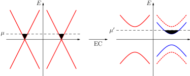
Figure 2: (color online) Schematic plot of the spin-down CDF bands before and after exciton condensation (EC) and exchange induced polarization.

In the case of $\nu=\pm 1/3$, these $\mathcal{K}$ matrices with $\widetilde{\phi}=2$ does not lead to the complete cancellation of the external magnetic field. Rather, the CDFs fill the Landau levels of the residual magnetic field $B^{*}=B-2|\rho|h/e$ at an integer filling. These CDF Landau levels will develop mass gaps through the statistical interaction and Coulomb interaction via magnetic catalyst at integer filling factors mc . Under exchange splitting, only one CDF Landau level will be completely filled and exhibits an integer QHE. This corresponds to a FQHE state at $\nu=\pm 1/3$ of the electrons Jain described by the single-component Laughlin state. In principle, other states at $\nu=q/(2pq\pm 1)$ can be constructed following the composite fermion approach Toke3 . Within the current framework, however, we can only study states within $\zeta LL$s due to the restriction that fictitious magnetic field generated through flux attachment must partially or completely cancel the external magnetic field.

Before turning to the pairing instability, we comment on the relation between magnetic catalysis and quantum Hall ferromagnetism. Recent experiments Dean ; Young2012 showed that SU(4) symmetry of the $n=\pm 1$ Landau levels is fully lifted. This seems to favor the quantum Hall ferromagnetism theories since magnetic catalysis cannot explain the extra plateaus at $\nu=\pm 3,\pm 5$. However, it is possible that the two mechanisms (magnetic catalysis and quantum Hall ferromagnetism) play leading roles in different regions and may even work in a collaborative way. For example, it is plausible that magnetic catalysis may be the driving force in the zeroth Landau levels while quantum Hall ferromagnetism is responsible for Landau level splitting beyond the zeroth Landau level. Furthermore, it was shown in Refs. Gorbar2002 ; Semenoff that the order parameters for these two mechanisms can both be nonzero.

IV Paired Quantum Hall States

We now show that, at even denominator filling fractions, the spin-valley polarized composite massive Dirac fermion liquid has a pairing instability where the quasiparticles on top of the exciton condensate form spin-triplet pairs in the chiral $p$-wave channel. In terms of the $R$-valley, the statistical pairing interaction is dominated by the $\ell=1$ angular momentum channel and has the form,

$$P_{\mathrm{st}}= -\frac{\pi}{\mathcal{V}}\sum_{s,\mathbf{k},\mathbf{p}}\mathcal{K}_{ss}\frac{\sin 2\varphi_{Rs\mathbf{k}_{>}}\cos 2\varphi_{Rs\mathbf{k}_{<}}}{k_{>}}$$

$$\quad\times e^{i(\theta_{\mathbf{k}}-\theta_{\mathbf{p}})}a^{\dagger}_{s\mathbf{k}}a^{\dagger}_{s-\mathbf{k}}a_{s-\mathbf{p}}a_{s\mathbf{p}}.$$ (37)

It is remarkable that this pairing interaction is present only if there is an exciton condensate, i.e., when $\varphi_{Rs\mathbf{k}}\neq 0$. Since the latter requires Landau level mixing, this implies that Landau level mixing is crucial for the pairing to occur. The variational wavefunction for the paired state has the BCS form $\ket{\Omega}=\prod_{\mathbf{k}}(u_{\mathbf{k}}+v_{\mathbf{k}}a^{\dagger}_{\mathbf{k}}a^{\dagger}_{-\mathbf{k}})\ket{0}$, with $|u_{\mathbf{k}}|^{2}+|v_{\mathbf{k}}|^{2}=1$, where $|0\rangle$ is the exciton vacuum defined in (III). Note that the variational wavefunction contains both the exciton and pairing order parameters which must be determined self-consistently by minimizing the ground state energy. The self-consistent equations for the dynamical mass have the same form as in (III) with $n^{R}_{\mathbf{k}}=|v_{\mathbf{k}}|^{2}$, but unlike in the normal state, exciton pairs exist even for $k<k^{R}_{F}$ due to pairing. The variation of the energy with respect to $u^{*}_{\mathbf{k}}$ and $v^{*}_{\mathbf{k}}$ leads to the familiar BdG equations (dropping the valley index),

$$E_{\mathbf{k}}u_{\mathbf{k}} =\xi_{\mathbf{k}}u_{\mathbf{k}}+\varDelta^{*}_{\mathbf{k}}v_{\mathbf{k}},$$

$$E_{\mathbf{k}}v_{\mathbf{k}} =-\xi_{\mathbf{k}}v_{\mathbf{k}}+\varDelta_{\mathbf{k}}u_{\mathbf{k}},$$ (38)

where $\xi_{\mathbf{k}}=\epsilon_{\mathbf{k}}-\beta_{\mathbf{k}}-\mu$, $E_{\mathbf{k}}=\sqrt{\xi^{2}_{\mathbf{k}}+|\varDelta_{\mathbf{k}}|^{2}}$, and $\beta_{\mathbf{k}}=g\frac{\pi}{\mathcal{V}}\sum_{\mathbf{p}}v_{0}(k,p)(1+n^{R}_{\mathbf{p}})$ comes from the Coulomb exchange. The gap function $\varDelta_{\mathbf{k}}$ is determined by the gap equation

$$\varDelta_{\mathbf{k}}= \frac{2\pi}{\mathcal{V}}\sum_{\mathbf{p}}e^{i(\theta_{\mathbf{k}}-\theta_{\mathbf{p}})}u^{*}_{\mathbf{p}}v_{\mathbf{p}}\left[\widetilde{\phi}\frac{1}{k_{>}}\frac{m_{\mathbf{k}_{>}}}{\epsilon_{\mathbf{k}_{>}}}\frac{\alpha_{\mathbf{k}_{<}}}{\epsilon_{\mathbf{k}_{<}}}\right.$$

$$- \left.\frac{g}{2}\left(1+\frac{m_{\mathbf{k}}m_{\mathbf{p}}}{\epsilon_{\mathbf{k}}\epsilon_{\mathbf{p}}}\right)v_{1}(k,p)-\frac{g}{2}\frac{\alpha_{\mathbf{k}}\alpha_{\mathbf{p}}}{\epsilon_{\mathbf{k}}\epsilon_{\mathbf{p}}}v_{0}(k,p)\right].$$

Fig. 3 displays the numerical solution of $E_{\mathbf{k}}$ and $\varDelta_{\mathbf{k}}$ at $\widetilde{\phi}=2$ and $g=0.3$, where the ground state is indeed a chiral $p+ip$ paired state. Because the Coulomb interaction is pair-breaking, the pairing gap $\Delta_{\mathrm{sc}}=2{\rm min}(E_{\mathbf{k}})$ reduces with increasing $g$ and vanishes at a critical value $g_{c}\approx 0.53$ and $1.28$ for $\widetilde{\phi}=2$ and $4$ respectively. For $g>g_{c}$, the massive Dirac fermions form a stable Fermi liquid state.

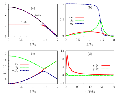
Figure 3: (color online) (a) The dynamical masses $m_{R\mathbf{k}}$ and $m_{L\mathbf{k}}$ in the chiral $p$-wave paired state. The corresponding exciton masses in the normal state are very close and drawn in dashed lines. (b) Solution of the BdG equation for the pairing gap function $\varDelta_{\mathbf{k}}$, the condensate amplitude $f_{\mathbf{k}}=u^{*}_{\mathbf{k}}v_{\mathbf{k}}$, and the momentum distribution function $n_{\mathbf{k}}$. (c) The CDF dispersion in the normal state and that of quasiparticle excitations in the paired state; (d) Pairing wave functions (unnormalized) in real space. All results are for $\widetilde{\phi}=2$ and $g=0.3$ with a momentum cutoff $\Lambda=2k_{F}$. Due to valley splitting, the Fermi vector is $k^{R}_{F}=\sqrt{2}k_{F}$.

To gain further insights into the paired state, we study the two-particle pairing wave function by projecting the BCS state to real space: $g(\mathbf{x}_{1}-\mathbf{x}_{2})=\braket{0}{\Psi(\mathbf{x}_{1})\Psi(\mathbf{x}_{2})}{\Omega}$. Because of the spinor structure, the upper and lower components are obtained separately,

$$g_{1}(\mathbf{x}) =\frac{1}{\mathcal{V}}\sum_{\mathbf{k}}\left(\cos\varphi_{R\mathbf{k}}+\sin\varphi_{R\mathbf{k}}\right)^{2}e^{-2i\theta_{\mathbf{k}}}e^{i\mathbf{k}\cdot\mathbf{x}}g_{\mathbf{k}},$$

$$g_{2}(\mathbf{x}) =\frac{1}{\mathcal{V}}\sum_{\mathbf{k}}\left(\cos\varphi_{R\mathbf{k}}-\sin\varphi_{R\mathbf{k}}\right)^{2}e^{i\mathbf{k}\cdot\mathbf{x}}g_{\mathbf{k}},$$ (39)

where $g_{\mathbf{k}}=v_{\mathbf{k}}/u_{\mathbf{k}}$. In the long wavelength limit, $g_{\mathbf{k}}\approx e^{i\theta_{\mathbf{k}}}/k$ and $m_{R\mathbf{k}}\approx m_{0}$ is essentially a constant (c.f. Fig. 3). We have, to quadratic order, $(\cos\varphi_{R\mathbf{k}}+\sin\varphi_{R\mathbf{k}})^{2}\approx 2-{v_{F}^{\prime}}^{2}k^{2}/2m^{2}_{0}$ and $(\cos\varphi_{R\mathbf{k}}-\sin\varphi_{R\mathbf{k}})^{2}\approx{v_{F}^{\prime}}^{2}k^{2}/2m^{2}_{0}$ where $v_{F}^{\prime}$ is the renormalized Fermi velocity. Thus, the large distance behaviors of the pairing wave function are $g_{1}(r)\propto 1/z+c\sqrt{2/\pi}\cos(\kappa r-\pi/4)/z\sqrt{r}$ and $g_{2}(r)\propto-c\sqrt{2/\pi}\cos(\kappa r-\pi/4)/\bar{z}\sqrt{r}$, where $c$ and $\kappa$ are numerical constants. The oscillatory terms in the above equations are due to the $k^{2}$ terms in the expansions, originating from the $k$ dependence of the mass, which should be distinguished from the oscillatory wave function in Ref. nonunitary . The many-body real space wave function for CDFs can be obtained by RG

$$\Psi_{\mathrm{CDF}}(\mathbf{x}_{1},\mathbf{x}_{2},\ldots,\mathbf{x}_{N})=\braket{0}{\Psi(\mathbf{x}_{1})\Psi(\mathbf{x}_{2})\ldots\Psi(\mathbf{x}_{N})}{\Omega}$$

$$=\frac{1}{2^{\frac{N}{2}}\left(\frac{N}{2}\right)!}\sum_{P}\mathrm{sgn}(P)\begin{pmatrix}\prod_{i=1}^{N/2}g_{1}(\mathbf{x}_{P(2i-1)}-\mathbf{x}_{P(2i)})\\ \prod_{i=1}^{N/2}g_{2}(\mathbf{x}_{P(2i-1)}-\mathbf{x}_{P(2i)})\end{pmatrix}$$

$$\approx\frac{1}{2^{\frac{N}{2}}\left(\frac{N}{2}\right)!}\sum_{P}\mathrm{sgn}(P)\begin{pmatrix}\prod_{i=1}^{N/2}1/(z_{P(2i-1)}-z_{P(2i)})\\ 0\end{pmatrix}.$$

where $N$ is an even number representing the number of CDFs. In the last line of the above equation, quadratic and higher order terms have been dropped. Note that except for the subleading oscillatory contributions that decay faster at large distances, the pairing wave function resides predominantly on one component of the spinor (i.e. on one of the sublattices) and has the form of the Moore-Read Pfaffian state in agreement with the numerical results shown in Fig. 3. It is remarkable that although the large holomorphic part on the upper component is indeed dominated by contributions from the $\zeta LL$ subspace, the wavefunction of the nonabelian ground state does not entirely lie in the $\zeta LL$ since the nonholomorphic, oscillatory contributions, although small, enter both the upper and the lower components of the wavefunction and can be attributed to the effects of Landau level mixing.

Similar to Ref. HLR ; Read95 , from the transformation in Eq. 11, the wave function for Dirac fermions is related to that of CDF by

$$\Psi_{\mathrm{MF}}(\mathbf{x}_{1},\ldots,\mathbf{x}_{N})=\prod_{i<j}\frac{(z_{i}-z_{j})^{\widetilde{\phi}}}{|z_{i}-z_{j}|^{\widetilde{\phi}}}\Psi_{\mathrm{CDF}}(\mathbf{x}_{1},\mathbf{x}_{2},\ldots,\mathbf{x}_{N}).$$

The full Jastrow factor $\prod_{i<j}(z_{i}-z_{j})^{\widetilde{\phi}}$ may be recovered by taken into account of fluctuations beyond mean field level Zhang92 .

V Conclusion

In this paper, we presented a composite relativistic fermion theory for the FQHE in graphene. We showed that the ground state has spontaneous spin-valley polarization, leading to a single-component Laughlin-like state at $\nu=1/3$ and a chiral $p$-wave pairing state of the Moore-Read Pfaffian at $\nu=1/2$. A crucial prediction of the present theory is the dynamical mass generation for the Dirac fermions through the formation of an exciton condensate in the zeroth Landau level. It originates from Landau level mixing and facilitates the spin-valley polarization and the pairing interaction for the paired states at even dominator filling fractions. This CDF mass, scaling with $\sqrt{B}$, should be detectable by scanning tunneling microscopy in high magnetic field. It would also be desirable to see if and how the inclusion of Landau level mixing affects the results of the numerical diagonalization studies Toke2 ; Wojs . In a recent experiment Ghahari on suspended graphene, a plateau like feature near $\nu=1/2$ is observed in some but not all samples. Future experiments are desirable to explore whether a true single-component quantum Hall state emerges at $\nu=1/2$ that would realize nonabelian statistics in graphene.

We end this paper by a few comments on some experimental results. For definiteness, we assumed near charge neutral state, the spin is polarized. A recent experiment Young2012 shows that the $\nu=0$ state is spin unpolarized. This suggests that the valley anisotropy is the dominant force behind the symmetry breaking near charge neutrality. This effect can be easily incorporated in the current framework by including a valley anisotropy term. In Ref. Dean , it is found that $\nu=5/3$ state is missing. This may be attributed to the different environment this state lies in. For $\nu=1/3$ state, the associated $\mathcal{K}$-matrix breaks the SU(4) symmetry. In contrast, the $\mathcal{K}$-matrix for $\nu=5/3$ preserves the symmetry. Due to the SU(4) symmetry, the associated Goldstone modes in $\nu=5/3$ may destabilize the state. A discussion of this issue can be found in Ref. Toke3 ; Abanin2013 . A more surprising result in Ref. Feldman1 is that the energy gaps are linear in $B$. Given that the energy scales in the problem are Coulomb interaction energy and Landau level spacing both scaling as $B^{1/2}$, any theory based on these energy scales should produce an energy gap that scales with $B^{1/2}$. Thus, this result presents a great puzzle. Further experimental and theoretical studies are needed to resolve it.

This work is supported in part by DOE grant DE-FG02-99ER45747, the NNSF of China, and the 973 program of MOST of China.

References

- (1) K.S. Novoselov et al, Science 306, 666 (2004).
- (2) K.S. Novoselov, A.K. Geim, S.V. Morozov, D. Jiang, M.I. Katsnelson, I.V. Grigorieva, S.V. Dubonos, and A.A. Firsov, Nature 438, 197 (2005).
- (3) Y. Zhang,Y.-W. Tan, H.L. Stormer and P. Kim, Nature 438, 201 (2005).
- (4) Y. Zhang, Z. Jiang, J.P. Small, M.S. Purewal, Y.-W. Tan, M. Fazlollahi, J.D. Chudow, J.A. Jaszczak, H.L. Stormer, and P. Kim, Phys. Rev. Lett. 96, 136806 (2006).
- (5) Z. Jiang, Y. Zhang, H.L. Stormer, and P. Kim, Phys. Rev. Lett. 99, 106802 (2007).
- (6) X. Du, I. Skachko, F. Duerr, A. Luican, and E.Y. Andrei, Nature 462, 192 (2009).
- (7) K.I. Bolotin, F Ghahari, M.D. Shulman, H.L. Stormer, and P. Kim, Nature 462, 196 (2009).
- (8) F. Ghahari, Y. Zhao, P. Cadden-Zimansky, K. Bolotin, and P. Kim, Phys. Rev. Lett. 106, 046801 (2011).
- (9) C.R. Dean, A.F. Young, P. Cadden-Zimansky, L. Wang, H. Ren, K. Watanabe, T. Taniguchi, P. Kim, J. Hone and K.L. Shepard, Nature Phys. 7, 693 (2011).
- (10) B.E. Feldman, B. Krauss, J.H. Smet, and A. Yacoby, Science 337, 1196 (2012).
- (11) B.E. Feldman, A.J. Levin, B. Krauss, D. Abanin, B.I Halperin, J.H. Smet, and A. Yacoby, arXiv:1303.0838.
- (12) V.P. Gusynin, V.A. Miransky and I.A. Shovkovy, Phys. Rev. Lett. 73, 3499 (1994); V.P. Gusynin, V.A. Miransky, S.G. Sharapov, and I.A. Shovkovy, Phys. Rev. B 74, 195429 (2006); E.V. Gorbar, V.P. Gusynin, V.A. Miransky, and I.A. Shovkovy, Phys. Rev. B 78, 085437 (2008).
- (13) K. Nomura and A.H. MacDonald, Phys. Rev. Lett. 96, 256602 (2006).
- (14) J. Alicea and M.P.A. Fisher, Phys. Rev. B 74 075422 (2006).
- (15) K. Yang, S. Das Sarma, and A.H. MacDonald, Phys. Rev. B 74, 075423 (2006).
- (16) V.M. Apalkov and T. Chakraborty, Phys. Rev. Lett. 97, 126801 (2006).
- (17) D.V. Khveshchenko, Phys. Rev. B 75, 153405 (2007);
- (18) C. Tőke, P.E. Lammert, V.H. Crespi, and J.K. Jain, Phys. Rev. B 74, 235417 (2006); C. Tőke and J.K. Jain, Phys. Rev. B 75, 245440 (2007).
- (19) M.O. Goerbig and N. Regnault, Phys. Rev. B 75, 241405(R) (2007).
- (20) Z. Papić, M.O. Goerbig, and N. Regnault, Phys. Rev. Lett. 105, 176802 (2010).
- (21) C. Tőke and J.K. Jain, Phys. Rev. B 76, 081403 (2007);
- (22) A. Wójs, G. Möller and N.R. Cooper, Acta Physica Polonica A 119, 592 (2011).
- (23) W. Bishara and C. Nayak, Phys. Rev. B 80, 121302(R) (2009).
- (24) A. Wójs, C. Tőke, and J.K. Jain, Phys. Rev. Lett. 105, 096802 (2010).
- (25) E.H. Rezayi and S.H. Simon, Phys. Rev. Lett. 106, 116801 (2011).
- (26) I. Sodemann and A.H. MacDonald, arXiv:1302.3896.
- (27) M.R. Peterson and C. Nayak, arXiv:1303.1541.
- (28) S.H. Simon and E.H. Rezayi, arXiv:1303.2809.
- (29) J.K. Jain, Phys. Rev. Lett. 63, 199 (1989).
- (30) B.I. Halperin, P.A. Lee, and N. Read, Phys. Rev. B 47, 7312 (1993).
- (31) N. Read, Semicon. Sci. Tech. 9, 1859 (1994).
- (32) S.-C. Zhang, Int. J. Mod. Phys. B6, 25 (1992).
- (33) J.E. Drut and T.A. Lähde, Phys. Rev. Lett. 102, 026802 (2009).
- (34) Y. Nambu and G. Jona-Lasinio, Phys. Rev. 122, 345 (1961).
- (35) X.-G. Wen and A. Zee, Phys. Rev. B 44, 274 (1991); Phys. Rev. B 46, 2290 (1992); Phys. Rev. Lett. 69, 1811 (1992).
- (36) W. Beugeling, M. O. Goerbig, and C. Morais Smith, Phys. Rev. B 81, 195303 (2010).
- (37) R. Rajaraman, Phys. Rev. B 56, 6788 (1997).
- (38) G. Moore and N. Read, Nucl. Phys. B 360, 362 (1991).
- (39) N. Read and D. Green, Phys. Rev. B 61, 10267 (2000).
- (40) Y.-M. Lu, Y. Yu, and Z. Wang, Phys. Rev. Lett. 105, 216801 (2010).
- (41) A.F. Young, C.R. Dean, L. Wang, H. Ren, P. Cadden-Zimansky, K. Watanabe, T. Taniguchi, J. Hone, K.L. Shepard, and P. Kim, Nature Physics 8, 550 (2012).
- (42) C. Töke and J.K. Jain, J. Phys.: Condens. Matter 24, 235601 (2012).
- (43) D.A. Abanin, B.E. Feldman, A. Yacoby, and B.I. Halperin, arXiv:1303.5372.
- (44) M.Z. Hasan and C.L. Kane, Rev. Mod. Phys. 82, 3045 (2010).
- (45) E.V. Gorbar, V.P. Gusynin, V.A. Miransky, I.A. Shovkovy, Phys. Rev. B 66, 045108 (2002).
- (46) G.W. Semenoff and F. Zhou, JHEP 1107, 037 (2011).