Spectral properties of the two-impurity Anderson model with varying distance and various interactions

Abstract

We present a novel approximation for the treatment of two interacting magnetic impurities immersed into a noninteracting metallic host. The scheme is based on direct perturbation theory with respect to the hybridization between the impurity and band electrons. This two-impurity enhanced noncrossing approximation can fully incorporate the indirect interactions between the impurities which are mediated by the conduction electrons as well as additional arbitrary direct interaction matrix elements. We qualify the approximation by investigating the uncoupled case and conclude the two-impurity approximation to be equally accurate as its single impurity counterpart. The physical properties of the two-impurity Anderson model (TIAM) are first investigated in some limiting cases. In a regime, where each of the uncoupled two impurities would exhibit a pronounced Kondo effect, we ignore the indirect coupling via the conduction band and only incorporate direct interactions. For a ferromagnetic direct exchange coupling, the system displays a behavior similar to a spin-one Kondo effect, while an antiferromagnetic coupling competes with the Kondo effect and produces a pseudogap in the many-body Kondo resonance of the single-particle spectral function. Interestingly, a direct one-particle hopping also produces a pseudogap but additionally pronounced side-peaks emerge. This gap is characteristically different from the case with antiferromagnetic coupling, since it emerges as a consequence of distinct Kondo effects for the bonding and anti-bonding orbital, i.e. it reflects a splitting of even and odd parity states. For the general case of only indirect coupling via the conduction band the results show signatures of all the previously discussed limiting cases as function of the impurity-impurity distance. Oscillatory behavior in physical quantities is to be expected due to the generated Ruderman-Kittel-Kasuya-Yosida (RKKY)-interaction. We are led to the conclusion that the well known Doniach-scenario captures essential aspects this model, but the details especially at small distances are more complicated.

I Introduction

The investigation of strong correlation effects plays a major role in contemporary condensed matter researchColeman (2003) as, for example, in the field of high-temperature cuprate superconductors,Plakida (2010) heavy-fermion systemsGrewe and Steglich (1991); *colemanHeavyFermionMag07; *steglich:HFQCP06; *siQCHF10 or frustrated magnetism.Lacroix et al. (2011) Due to the complexity of the phenomena and the theoretical models there are still fundamental questions to be addressed, despite long and intensive research in these fields.

Quite generally, the reason for this can be found in the presence of competing physical tendencies, whose characteristic energy scales are close together.Dagotto (2005) Then, a very rich variety of physical scenarios results since subtle differences in the external conditions or small parameter changes can tip the balance from one dominating mechanism to another.

We consider the two-impurity Anderson modelAlexander and Anderson (1964) (TIAM) as one of the most basic models incorporating such competing interactions. There, two magnetic impurities are immersed with finite distance into a host with a noninteracting conduction band and hybridizations between conduction electrons and local interacting electrons.

A single impurity is prone to the Kondo effect,Hewson (1993) where an effective antiferromagnetic exchange between the conduction electrons and the local spin of the magnetic impurity leads to a dynamic spin-screening. This archetypical many-body effect is associated with an characteristic energy scale $T_{\mathrm{K}}$ (Kondo scale) which is nonanalytic and exponentially small in terms of the effective exchange.

Additionally, the noninteracting band electrons induce an effective magnetic exchange between the two impurities,Ruderman and Kittel (1954); *yosidaRKKY57; *kasuyaRKKY56 known as the Ruderman-Kittel-Kasuya-Yosida (RKKY)-interaction. This RKKY-exchange can be ferromagnetic or antiferromagnetic, depending on the spatial separation of the two impurities.

The RKKY-exchange is expected to be dominant for a small hybridization between the impurity and the conduction band and favors an inter-impurity coupling of the spins usually associated with long-ranged magnetic order. The Kondo coupling, on the other hand, strongly increases toward larger hybridization strengths and promotes individual Kondo effects at each impurity resulting in two uncoupled and screened impurities. This scenario proposed by DoniachDoniach (1977) for the competition between these two mechanisms is at the heart of the rich variety observed in many physical systems.Grewe and Steglich (1991); *colemanHeavyFermionMag07; *steglich:HFQCP06; *siQCHF10

The TIAM as the simplest model for this competition has be studied intensively Jayaprakash et al. (1981); *PhysRevLett.58.843; *jones:twoImpurityKondo88; Sakai et al. (1990); *PhysRevB.35.4901; *PhysRevLett.72.916; *PhysRevB.59.85; *PhysRevB.65.140405; *Sakai1993323; *Nishimoto2006; *hattoriTIAM07; *mrossTIAM08; *leeTwoImp10; Silva et al. (1996); Zhu and Zhu (2011) in the past and has been realized in a recent experiment.Bork et al. (2011) The thermodynamic properties of the model are governed by a quantum critical point separating the ordered and paramagnetic (Kondo) ground states in case of identical impurities and particle-hole symmetry.Jones and Varma (1987); *jones:twoImpurityKondo88 However, the quantum critical point is unstable and turns into a crossover once one of these symmetries is broken or a direct hopping is included.Sakai et al. (1990); Silva et al. (1996); Zhu and Zhu (2011) The dynamic properties under general conditions, that is varying impurity-impurity distance, hybridization and interaction strength, are not as clear. Especially the situation with finite non-diagonal hybridization is not well studied since usually the RKKY exchange is simulated via a direct exchange interaction.

In this work we present an approach to the a general TIAM which is formulated in the framework of direct perturbation theory in the hybridizationKeiter and Kimball (1970); *grewe:IVperturb81; *Grewe:lnca83; *keiterMorandiResolventPerturb84 which utilizes skeleton graphs for families of time ordered diagrams. These techniques have been laid out in the literature, e.g. in connection with the Kondo effect or the mixed valence problem,Kuramoto and Müller-Hartmann (1985); *bickers:nca87a and have served to define approximation schemes of great usefulness and quality.Grewe et al. (2008); *schmittSus09; Kroha and Wölfle (2005)

There have already been approaches to the TIAM with these techniques,Schiller and Zevin (1993); *Schiller1996 but these were restricted to infinite Coulomb interaction, $U\to\infty$, neglected vertex corrections, and ignored non-diagonal ionic propagators (see below for details). The present scheme is an extension of the finite-$U$ enhanced noncrossing approximation (ENCA)Pruschke and Grewe (1989), which improves on the well known noncrossing approximation (NCA)Grewe (1983b); *Kuramoto:ncaI83 by the inclusion of low-order vertex corrections. It is also a direct extension of the ENCA for the multi-orbital situation as described in Ref. Grewe et al., 2009.

Apart from an application to the rich and interesting physics encountered in the TIAM, our new two-impurity solver also is of interest for extensions of the dynamical mean-field theory to include nonlocal two-site correlations. Compared to other existing two-impurity solvers the present scheme has some advantages as well as shortcomings: Like all the schemes based on perturbation theory in the hybridization, it has some problems to correctly describe the Fermi liquid properties at very low temperatures. This does not represent a major drawback as many scenarios and questions of current interest can be addressed at temperatures accessible within these schemes (see, for example, Ref. Schmitt, 2010; *greteKink11; *schmittMagnet12). As will be demonstrated below and as it is known from the single-impurity case,Pruschke and Grewe (1989); Grewe et al. (2008); *schmittSus09; Grewe et al. (2009) these schemes correctly describe the non-perturbative Kondo-physics and are able to reproduce the exponentially small low-energy Kondo scale. Additionally, there are no adjustable parameters and this theory is directly formulated for correlation functions at the real frequency axis This avoids the inaccuracies connected with a numerical analytic continuation of imaginary time data, as obtained, for example, from quantum Monte Carlo schemes.

II Model

We consider two impurities (labeled as $f$-electrons) placed at at lattice sites $\underline{R}_{j}$ with $j=\{1,2\}$. That part of the Hamiltonian preserving all local occupation numbers is

$$\hat{H}^{f}_{0}= \sum_{j,\sigma}\epsilon^{f}_{j\sigma}\hat{n}_{j\sigma}^{f}+\sum_{j=\{1,2\}}U_{j}\hat{n}^{f}_{j\uparrow}\hat{n}^{f}_{j\downarrow}$$

$$+\frac{1}{2}\sum_{l\neq j,\sigma,\sigma^{\prime}}U^{\prime}_{12}\hat{n}^{f}_{j\sigma}\hat{n}^{f}_{l\sigma^{\prime}}.$$ (1)

The operators $\hat{f}^{\phantom{\dagger}}_{j\sigma}$ and ${\hat{f}}^{\dagger}_{j\sigma}$ are the usual annihilation and creation operators for impurity $f$-electrons with spin $\sigma=\{+,-\}=\{\uparrow,\downarrow\}$ at the lattice $j$ and $\hat{n}_{j\sigma}^{f}={\hat{f}}^{\dagger}_{j\sigma}\hat{f}^{\phantom{\dagger}}_{j\sigma}$. The density-density Coulomb interaction is incorporated via the matrix elements $U_{j}$ for on-site and $U^{\prime}_{12}$ for inter-site interaction. We also allow for more general couplings between the two impurities

$$\hat{W}^{f}= \sum_{l\neq j\sigma}t_{lj}{\hat{f}}^{\dagger}_{l\sigma}\hat{f}^{\phantom{\dagger}}_{j\sigma}-\frac{1}{2}\sum_{l\neq j}J_{lj}\underline{\hat{S}}^{f}_{l}\underline{\hat{S}}^{f}_{j}+\hat{W}^{\prime}(X,Y),$$ (2)

where the first term is direct single-particle hopping with amplitude $t_{lj}$ and the second term a Heisenberg exchange with exchange coupling $J_{lj}$ and $\underline{\hat{S}}_{j}^{f}$ the vector $f$-electron spin operator. The third term allows, e.g., correlated hopping (associated with matrix element $X$) and pair-hopping (associated with matrix element $Y$).

These impurities are immersed into a lattice with a noninteracting conduction band ($c$-electrons) with the dispersion relation $\epsilon^{c}_{\underline{k}}$,

$$\hat{H}^{c}_{0}= \sum_{\underline{k},\sigma}\epsilon^{c}_{\underline{k}}\hat{n}_{\underline{k}\sigma}^{c}$$ (3)

with the number operator for $c$-electrons $\hat{n}_{\underline{k}\sigma}^{c}=\hat{c}^{\dagger}_{\underline{k}\sigma}\hat{c}^{\phantom{\dagger}}_{\underline{k}\sigma}$ with spin $\sigma$ and crystal momentum $\underline{k}$. Both subsystems hybridize via a term

$$\hat{V}= \sum_{j,\underline{k},\sigma}\left(V_{\underline{k}}e^{-i\underline{k}\,\underline{R}_{j}}\hat{c}^{\dagger}_{\underline{k},\sigma}\hat{f}^{\phantom{\dagger}}_{j\sigma}+h.c.\right).$$ (4)

The total Hamiltonian then reads

$$\hat{H} =\hat{H}_{0}^{f}+\hat{W}^{f}+\hat{H}_{0}^{c}+\hat{V}.$$ (5)

Even though in principal there is no limitation in applying our calculational scheme to this model in full generality, in this work we will mostly consider identical impurities and focus on the half-filled particle-hole symmetric case, where two electrons are placed in the two-impurity cluster.

III Novel two-impurity solver based on direct perturbation theory

The general idea of direct perturbation theory is to treat the two-impurity subsystem $\hat{H}_{0}^{f}+\hat{H}_{0}^{c}+\hat{W}^{f}$ exactly and to use $\hat{V}$ as the perturbation. With $\hat{W}^{f}=\hat{V}=0$ the Fock-space of $f$-electrons is diagonalized in terms of the local occupation numbers $\hat{n}^{f}_{j\sigma}$. An eigenbasis of $\hat{H}_{0}^{f}$ is generated by all product states with the factors taken from the two versions of the local $f$-eigenbasis for the two sites $j=1$ and $2$ , respectively

$$|0\rangle\phantom{{}_{j}} \equiv|n^{f}_{j\uparrow}=n^{f}_{j\downarrow}=0\rangle$$ (6)

$$|\!\!\uparrow\rangle_{j} \equiv|n^{f}_{j\uparrow}=1,n^{f}_{j\downarrow}=0\rangle={\hat{f}}^{\dagger}_{j\uparrow}|{0}\rangle$$

$$|\!\!\downarrow\rangle_{j} ={\hat{f}}^{\dagger}_{j\downarrow}|{0}\rangle$$

$$|2\rangle_{j} ={\hat{f}}^{\dagger}_{j\uparrow}{\hat{f}}^{\dagger}_{j\downarrow}|{0}\rangle$$

The inclusion of the term $\hat{W}^{f}$ makes it necessary to transform to a different many-electron eigenbasis of $f$-states in order to diagonalize the two-impurity subsystem. The following discussion of the novel two-impurity solver is formulated in general terms. It uses the afore mentioned multi-electron eigenstates of the diagonalized $f$-system,

$$\hat{H}_{0}^{f}|M\rangle =E_{M}|M\rangle,$$ (7)

labeled by quantum numbers $M$. The corresponding Hubbard-transfer operators

$$\hat{X}_{MM^{\prime}} =|M\rangle\langle M^{\prime}|$$ (8)

allow for the decomposition of one-particle creation- and annihilation operators (with coefficients specified later),

$$\hat{f}^{\phantom{\dagger}}_{j\sigma} =\sum_{\begin{subarray}{c}M,M^{\prime}\end{subarray}}\alpha^{j\sigma}_{MM^{\prime}}\hat{X}_{MM^{\prime}},$$ (9)

$${\hat{f}}^{\dagger}_{j\sigma} =\sum_{\begin{subarray}{c}M,M^{\prime}\end{subarray}}\left(\alpha^{j\sigma}_{MM^{\prime}}\right)^{*}\hat{X}_{M^{\prime}M}.$$

In direct perturbation theory the partition function and the fermionic two-point Green functions are expressed as contour integrals in the complex energy plane:Keiter and Kimball (1970); *grewe:IVperturb81; *Grewe:lnca83; *keiterMorandiResolventPerturb84

$$\mathcal{Z} =\oint_{\mathcal{C}}\frac{dz}{2\pi i}e^{-\beta z}\mathrm{Tr}\left[\mathcal{\hat{R}}(z)\right]$$ (10)

$$=\mathcal{Z}_{c}\sum_{M}\int\limits_{-\infty}^{\infty}d\omega e^{-\beta\omega}\left[-\frac{1}{\pi}\mathrm{Im}P_{M;M}(\omega+i\delta)\right],$$

$$G_{\scriptscriptstyle{\hat{A},\hat{B}}}(i\omega_{n})=\frac{1}{\mathcal{Z}}\oint\limits_{\begin{subarray}{c}\mathcal{C}\end{subarray}}\frac{dz}{2\pi i}e^{-\beta z}\mathrm{Tr}\left[\mathcal{\hat{R}}(z)\;\hat{A}\;\mathcal{\hat{R}}(z+i\omega_{n})\;\hat{B}\right]$$

$$\phantom{M}=\frac{1}{\mathcal{Z}_{f}}\sum_{\begin{subarray}{c}M^{\prime},M^{\prime\prime},\\ M^{\prime\prime\prime},M\end{subarray}}\alpha_{M^{\prime},M^{\prime\prime}}^{A}\alpha_{M^{\prime\prime\prime},M}^{B}\oint_{\mathcal{C}}\frac{dz}{2\pi i}e^{-\beta z}\times$$ (11)

$$\phantom{M}\times P_{\scriptscriptstyle{M;M^{\prime}}}(z)\Lambda_{\scriptscriptstyle{M^{\prime};M^{\prime\prime}}}(z,z+i\omega_{n})P_{\scriptscriptstyle{M^{\prime\prime};M^{\prime\prime\prime}}}(z+i\omega_{n}).$$

with the resolvent operator $\mathcal{\hat{R}}(z)=\left[z-\hat{H}\right]^{-1}$ and $\mathcal{Z}_{c}=\mathrm{Tr}_{c}\left(e^{-\beta\hat{H}_{c}}\right)$ is the partition function of the noninteracting subsystem of band electrons. The $P_{M,M^{\prime}}(z)$ are so-called ionic propagators which capture the correlated dynamics of a transition from an ionic $f$-state with quantum number $M^{\prime}$ to a state with $M$. These are exact equations if the exact vertex functions $\Lambda_{\scriptscriptstyle{M^{\prime};M^{\prime\prime}}}(z,z+i\omega_{n})$ are used. In practice, however, the exact vertex functions are unknown and approximations for $\Lambda_{\scriptscriptstyle{M^{\prime};M^{\prime\prime}}}$ are employed.

For simplicity, we will confine our considerations to one-particle $f$-Green functions where $\hat{A}=\hat{f}^{\phantom{\dagger}}_{j\sigma}$ and $\hat{B}={\hat{f}}^{\dagger}_{l\sigma^{\prime}}$. For the two-impurity model the one-particle Green function is conveniently written as a $2\times 2$ matrix for each spin component,

$$\underline{\underline{G}}_{\sigma}=\left(\begin{array}[]{cc}G_{\hat{f}^{\phantom{\dagger}}_{1\sigma},{\hat{f}}^{\dagger}_{1\sigma}}&G_{\hat{f}^{\phantom{\dagger}}_{1\sigma},{\hat{f}}^{\dagger}_{2\sigma}}\\ G_{\hat{f}^{\phantom{\dagger}}_{2\sigma},{\hat{f}}^{\dagger}_{1\sigma}}&G_{\hat{f}^{\phantom{\dagger}}_{2\sigma},{\hat{f}}^{\dagger}_{2\sigma}}\\ \end{array}\right).$$ (12)

A central quantity of physical interest is the one-particle spectral function which is given by the diagonal part of the Green function,

$$\rho^{f}_{j}(\omega)=-\frac{1}{\pi}\mathrm{Im}G_{\hat{f}^{\phantom{\dagger}}_{j\sigma},{\hat{f}}^{\dagger}_{j\sigma}}(\omega+i\delta),$$ (13)

where the limit $0<\delta\to 0$ is implied.

In contrast to what is commonly needed for (effective) single-impurity models,Grewe (1983b); *Kuramoto:ncaI83; Grewe et al. (2008) we introduced non-diagonal ionic propagators,

$$P_{M;M^{\prime}}(z)=\sum_{\begin{subarray}{c}\mathrm{conduction}\\ \;\;\mathrm{states}\;\gamma\end{subarray}}\frac{e^{-\beta E_{\gamma}}}{\mathcal{Z}_{c}}\langle\gamma,M|\mathcal{\hat{R}}(z+E_{\gamma})|M^{\prime},\gamma\rangle$$ (14)

which together with the diagonal components and the vertex functions $\Lambda_{M;M^{\prime}}(z,z^{\prime})$ are the central quantities of interest which need to be computed.

The perturbational processes contributing to the ionic propagators and vertex functions take place along the imaginary time axis $0\leq\tau<\beta\equiv\frac{1}{T}$. These processes can be partially summed-up to families of time-rotated diagrams on cylinders where the endpoints $\tau=0$ and $\tau=\beta$ are identified. The Green function of Eq. (III) is represented by one particular diagram where the external line (accounting for the operator $\hat{B}$) is attached to a bare vertex occuring at the latest time; the dressed vertex $\Lambda_{M,M^{\prime}}(z,z^{\prime})$, where the external line associated with the operator $\hat{A}$ is attached, occurs at an earlier time. The initial and final ionic state $M$ is displayed twice in graphical representations for clarity, but is included only once in the corresponding formulas.

As usual, propagators are favorably built up from irreducible self-energies $\Sigma_{M;M^{\prime}}(z)$, which together with the vertex functions form a closed set of skeleton equations. Diagrammatic contributions to the self-energies are identified as pieces of diagrams which cannot be separated into disjoint parts by cutting only the time axis of each site in the cluster.

It is important to realize here, that the time-ordered processes, generated by expanding the resolvents in Eq. (14) in terms of the hybridization $\hat{V}$, generally extend over all sites of the cluster. Local pieces on one particular site $j$ can occur in proper time-order, either after an electron has is transferred from a different site $l$ or after an interaction process, both induced by $\hat{W}^{f}$. If $\hat{W}^{f}$ would have been regarded as a perturbation, too, these events would appear in the diagrams explicitly. However, we will take $\hat{W}^{f}$ into account exactly via a non-diagonal form of the ionic propagators $P^{(0)}_{M;M^{\prime}}(z)$, which corresponds to the unperturbed Hamiltonian $\hat{H}^{f}_{0}+\hat{H}^{c}_{0}+\hat{W}^{f}$.

As a consequence of the all-embracing unique time-order in the cluster only one energy variable is present after the Laplace-transform. Another consequence of this fact concerns the dynamical interdependence of local parts of a process in a cluster. As already mentioned, all events occur in a definite time-order. Even if two processes happen to be located at separate impurities, e.g. the excitation of two band electrons and re-absorption at the respective same site, different time-orderings of the individual two excitations and absorptions are counted separately in this approach. For example, interchanging the emission times of the two processes generates or removes one crossing of two band-electron lines. As the approximation is organized in numbers of crossing band electron lines higher-order vertex corrections with a multitude of crossing lines are not included. This introduces artificial inter-site correlations.

Therefore, all such approximations within a two-impurity model will in principle not faithfully reduce to two independent sites in the case of uncoupled impurities. They have to be thoroughly checked in the limiting case of two independent sites, where an ordinary Kondo effect is expected at each site. As it turns out, the two-impurity solvers to be introduced below are capable of describing this limiting case reasonably well. On the other hand, these approximation schemes will perform even better when real physical inter-site correlations make it necessary to respect overall time order.

The connection between the irreducible self-energies and the ionic propagators is provided by a Dyson-equation

$$P_{M;M^{\prime}}(z)= P^{(0)}_{M;M^{\prime}}(z)$$ (15)

$$+\sum_{M^{\prime\prime},M^{\prime\prime\prime}}P^{(0)}_{M;M^{\prime\prime}}\Sigma_{M^{\prime\prime};M^{\prime\prime\prime}}(z)P_{M^{\prime\prime\prime};M^{\prime}}(z).$$

As already stated above, the action of $\hat{W}^{f}$ is included in $P^{(0)}_{M;M^{\prime}}$, i.e. it is a solution to the equation

$$P^{(0)}_{M;M^{\prime}}(z) =\frac{1}{z-E_{M}}\delta_{M,M^{\prime}}$$ (16)

$$\phantom{=}+\frac{1}{z-E_{M}}\sum_{M^{\prime\prime}}\langle\hat{W}^{f}\rangle_{M,M^{\prime\prime}}^{\phantom{{(0)}}}P^{(0)}_{M^{\prime\prime};M^{\prime}}(z).$$

The irreducible self-energy $\Sigma_{M;M^{\prime}}$ incorporates the additional modifications brought about by the hybridization $\hat{V}$. The limit of an isolated cluster not hybridizing with the conduction band is thereby exactly reproduced for vanishing hybridization with the band states, since

$$\qquad V_{\underline{k}}\to 0:\quad\Sigma_{M;M^{\prime}}(z)\to 0.$$ (17)

For the present case of a cluster with two sites $j=1,2$ and $s$-shells only, the quantum numbers are specified as $M=\left(m_{1},m_{2}\right)$ with $m_{j}=\{0,\uparrow,\downarrow,2\}$. The annihilation operators of Eq. (9) are then given as

$$\hat{f}^{\phantom{\dagger}}_{1\sigma}= \big{[}|0\rangle_{1}{}_{1}\!\langle\sigma|+\sigma|-\sigma\rangle_{1}{}_{1}\!\langle 2|\big{]}\otimes\hat{1}_{2},$$ (18)

$$\hat{f}^{\phantom{\dagger}}_{2\sigma}= \hat{1}_{1}\otimes\big{[}|0\rangle_{2}{}_{2}\langle\sigma|+\sigma|-\sigma\rangle_{2}{}_{2}\!\langle 2|\big{]},$$

$$\hat{1}_{j}= |0\rangle_{j}{}_{j}\langle 0|+(-1)^{j}\sum_{\begin{subarray}{c}\sigma\end{subarray}}|\sigma\rangle_{j}{}_{j}\!\langle\sigma|+|2\rangle_{j}{}_{j}\!\langle 2|.$$

The differing sign in the definition of the local identity operators for impurity 1 and 2 stems from the definition of the basis states, in particular from the prescribed order in which the creation operators act to produce the other basis state from the two-site vacuum.

The overall sign of a diagram turns out to be more subtle for the two-impurity case than for a single-impurity. In the latter the overall sign is determined by simply including a factor of $(-1)$ for each crossing of two band electron lines. For the two-impurity case, we have found no better way than to count all exchange processes of Fermi-operators in the course of reducing expectation values of operator products to normal order. This is done algorithmically on a computer along with the enumeration and classification of all different diagrams contribution to the quantity of interest.

The analytic contributions are visualized in a diagrammatic language similar to the one developed long ago for the single-impurity problem,Keiter and Kimball (1971) however, with a few characteristic differences. Even though there exists only one energy variable $z$ for both sites, we distinguish two vertical lines corresponding to local processes on sites 1 (left) and 2 (right) for clarity. These become decorated with vertices ordered along the vertical direction due to hybridization events. Bare vertices are depicted as circles with the corresponding number of the site where the external line is attached at, and dressed vertices are depicted as triangles; they embrace both lines as shown in Fig. 1(a) and (b).

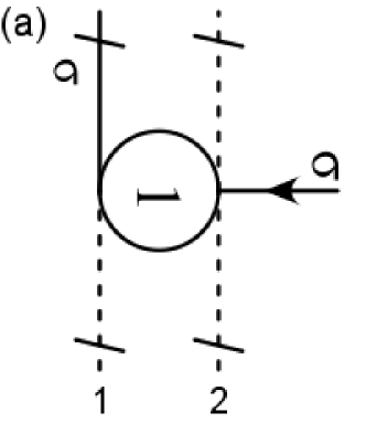
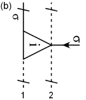
Figure 1: (a) Bare vertex depicting an absorption of a band electron with spin $\sigma$ at site 1, changing the two-impurity quantum number from $M=(0,0)$ to the $M^{\prime}=(\sigma,0)$. (b) Dressed vertex for the absorption of a band electron with spin $\sigma$ at site $i$. The left (right) vertical line denotes site 1 (site 2) and the incoming arrow a band electron. A dashed vertical line represents an empty and a full vertical line a singly occupied shell, where the spin of the electron is indicated next to the line. The number in the vertex symbol denotes the site, to which the band electron line is attached. For the bare vertex this can occur only on site 1, while for the dressed vertex this is not specified. In an analytic expression, the bare vertex amounts to a factor of $1$, while the dressed vertex stands for the function $\Lambda_{00;0\sigma}^{i}(z,z+\epsilon)$, when the band electron has an energy $\epsilon$ and the local two-site cluster has the complex energy variable $z$.

Figure 2: Contributions to the self-energy $\Sigma_{00;00}(z)$. The squares represent ionic propagators, $P_{m_{f1}m_{f2};m_{i1}m_{i2}}(z)$, where the earlier [later] state characterized by the quantum numbers $M=(m_{i1},m_{i2})$ [$M=(m_{f1},m_{f2})$] is indicated by the attached lower [upper] two lines. For clarity, a diagonal line inside the box is added in case of a non-diagonal propagator. Summations over all internal quantum numbers is understood in all graphs presented in this work.

The ionic propagators between vertices are nonlocal objects and non-diagonal in quantum numbers $M$, and as such they describe the combined time evolution of both ionic states. Band-electron lines are always considered to be external to the whole cluster and can be tied to either of both sites indicated by the number inside the vertex symbol. The short horizontal lines denote amputation as usual, where the initial and final states are not included in the analytical representations. The translation of a diagram into an analytical expression is handled in complete analogy to the diagrammatic rules stated in the literature,Keiter and Kimball (1970); *grewe:IVperturb81; *Grewe:lnca83; *keiterMorandiResolventPerturb84; Kuramoto and Müller-Hartmann (1985); *bickers:nca87a except for the sign rule mentioned above.

Hybridization events occur as diagonal ($j=l$) and non-diagonal ($j\neq l$) processes characterized by the (complex) functions

$$\Gamma_{j,l}(z)=\frac{1}{N}\sum_{\underline{k}}\frac{|V_{\underline{k}}|^{2}e^{i\underline{k}\;\left(\underline{R}_{l}-\underline{R}_{j}\right)}}{z-\epsilon_{\underline{k}}}.$$ (19)

Their imaginary part at the real frequency axis ($z=\omega\pm i\delta$)

$$\Delta_{j,l}(\omega) =\frac{1}{2i}\big{[}\Gamma_{j,l}(\omega-i\delta)-\Gamma_{j,l}(\omega+i\delta)\big{]}$$ (20)

$$=\frac{1}{N}\sum_{\underline{k}}|V_{\underline{k}}|^{2}e^{i\underline{k}\;\left(\underline{R}_{l}-\underline{R}_{j}\right)}\pi\delta(\omega-\epsilon_{\underline{k}})$$

is called hybridization function and is the physically most relevant part. The diagonal component at zero frequency corresponds to the well-known Anderson width of a resonant impurity level, $\Delta\equiv\Delta_{jj}(\omega=0)$. As with the other quantities, the diagonal and non-diagonal components are conveniently treated as matrices.

We refrain from presenting the complete system of self-energy and vertex-equations, which even after using all symmetries of the two-site Anderson-model, is far too large to present (It can be found, however, in Ref. Jabben, 2010.) Instead we exemplify the structure by selected examples for self-energy and vertex equations.

The cluster vacuum with no electrons on each of the two ionic shells experiences excitations according to the self-energy diagrams shown in Fig. 2. The corresponding analytic contribution is

$$\Sigma_{00;00}(z) =\sum\limits_{i,\sigma}\int\limits_{-\infty}^{\infty}\frac{d\epsilon}{\pi}\Big{[}$$ (21)

$$\phantom{-}\Delta_{i,2}(\epsilon)f(\epsilon)\;\Lambda_{00;0\sigma}^{i}(z,z+\epsilon)\;P_{0\sigma;0\sigma}(z+\epsilon)$$

$$+\Delta_{i,1}(\epsilon)f(\epsilon)\;\Lambda_{00;0\sigma}^{i}(z,z+\epsilon)\;P_{0\sigma;\sigma 0}(z+\epsilon)$$

$$+\Delta_{i,2}(\epsilon)f(\epsilon)\;\Lambda_{00;0\sigma}^{i}(z,z+\epsilon)\;P_{\sigma 0;0\sigma}(z+\epsilon)$$

$$+\Delta_{i,1}(\epsilon)f(\epsilon)\;\Lambda_{00;0\sigma}^{i}(z,z+\epsilon)\;P_{\sigma 0;\sigma 0}(z+\epsilon)\Big{]}.$$

Among the graphical elements in Fig. 2 is an insertion with a diagonal line inside the square. This represents a non-diagonal ionic propagator where an electron is transferred from one site of the cluster to the other. Figure 3 presents the diagrammatic contributions to a non-diagonal self-energy.

Figure 3: Contributions to the self-energy $\Sigma_{\sigma 0;0\sigma}(z)$. The double-line visible in some contributions indicates a doubly occupied ionic shell on one site.

Up to now, all the equations for propagators and self-energies are exact. However, the dressed vertex functions, as indicated by the triangles in the graphs, have not been specified yet. Clearly, the exact vertex functions are in general unknown and approximations have to be introduced.

The simplest approximation amounts to ignoring all vertex corrections and just replacing every full vertex by a bare one, that is $\Lambda_{M;M^{\prime}}^{j}\to 1$. The result is the natural generalization of the NCA for finite $U$ (usually termed SNCA) to the two-impurity case and will be referred to as two-impurity SNCA.

In order to incorporate the correct order of magnitude for the Schrieffer-Wolff exchange coupling for finite $U$, the first order vertex corrections with one crossing of band electron lines have to be included.Pruschke and Grewe (1989) The extension of this ENCA for the single-impurity to the present two-impurity set-up will be termed two-impurity ENCA. As an example we present the vertex function $\Lambda_{00;\sigma 0}^{i}(z,z^{\prime})$ within the two-impurity ENCA in Fig. 4.

Figure 4: Contributions to the vertex $\Lambda_{00;\sigma 0}^{1}$ within the two-impurity ENCA approximation which includes the first oder of vertex corrections.

A closed system of coupled equations for ionic propagators, self-energies and vertex functions includes many such integral equations. Great care is needed to identify all different processes together with the proper assignment of quantum numbers, energies, matrix elements and signs. This coupled system is solved self-consistently for the unknown self-energies and ionic propagators. There are between 6 and 158 different ionic propagators, depending on symmetries, and about 10-100 different diagrammatic contributions to each self-energy. Therefore, the number of necessary convolutions in each iteration step is easily in the thousands. As in the usual procedure, an additional set of coupled integral equations has to be solved for the so-called defect propagators.Kuramoto and Kojima (1984); Grewe et al. (2008); *schmittSus09

While the computational effort for the two-impurity schemes presented here is increased considerably compared to their single-impurity counterparts, the numerical difficulties are of the same nature: The ionic propagators exhibit very narrow features near the ionic thresholds which can be handled by the usage of optimally adapted energy meshes. The strongest challenge is posed by the numerical solution of the system of equations for the defect propagators. The lack of an absolute scale, i.e. the lack of the knowledge of the partition function, leads to suboptimal convergence properties.Schmitt (2009); Jabben (2010) However, proper and rather accurate solutions can indeed be obtained, and results will be presented in the following sections. The interested reader can consult Refs. Jabben, 2010 and Schmitt, 2009 for more details.

When extending these approximations to systems with more local orbitals or impurities one is confronted with the fundamental problem of an exponentially increasing number of local many-body states. Additionally, the inclusion of vertex corrections as in the two-impurity ENCA further increases the contributions to each ionic self-energy. However, in the present approach symmetries can easily be implemented by identifying equivalent propagators; thus, the computational cost is dramatically reduced. In this respect it is also very effective and easily implemented to restrict the allowed local occupation and to exclude many-body states with very high excitation energies, as it was done for the two-orbital Anderson model (Ref. Grewe et al., 2009).

IV Results for uncoupled impurities

In this section we first concentrate on the basic question of how the novel two-impurity solver performs in some simple model situations. We compare the two-impurity SNCA and ENCA with the corresponding SNCA- and ENCA-solutions of the single-impurity Anderson problem in order to check on the presence and relative weight of artificial correlations introduced by the two-impurity treatment.

We assume spin-degeneracy in the following and measure energies with reference to the chemical potential $\mu=\omega=0$. We always take the noninteracting conduction electrons to have the tight-binding dispersion of a three-dimensional simple-cubic lattice

$$\epsilon_{\underline{k}}^{c}=-2t\big{[}\cos(k_{x})+\cos(k_{y})+\cos(k_{z})\big{]}$$ (22)

(with the lattice spacing set to one, $a=1$). As the unit of energy we take either the half-bandwidth of the noninteracting conduction band, $D=6t$, or the Anderson width $\Delta$, depending on what seems more appropriate. We also restrict ourselves to identical impurities, that is $\epsilon^{f}_{1}=\epsilon^{f}_{2}=\epsilon^{f}$, $U_{1}=U_{2}=U$, and $\rho^{f}\equiv\rho^{f}_{j}$ and mostly focus on the two-electron sector.

We define even ($+$) and odd ($-$) parity one-particle statesJayaprakash et al. (1981)

$$\hat{f}^{\phantom{\dagger}}_{\pm\sigma}=\frac{1}{\sqrt{2}}(\hat{f}^{\phantom{\dagger}}_{1\sigma}\pm\hat{f}^{\phantom{\dagger}}_{2\sigma})$$ (23)

and also introduce even and odd hybridization functions,

$$\Delta_{+}(\omega) =\frac{2}{N}\sum_{\underline{k}}|V_{\underline{k}}|^{2}\cos^{2}\big{(}\frac{1}{2}\underline{k}\;\underline{d}\big{)}\pi\delta(\omega-\epsilon^{c}_{\underline{k}})$$ (24)

$$\Delta_{-}(\omega) =\frac{2}{N}\sum_{\underline{k}}|V_{\underline{k}}|^{2}\sin^{2}\big{(}\frac{1}{2}\underline{k}\;\underline{d}\big{)}\pi\delta(\omega-\epsilon^{c}_{\underline{k}}).$$ (25)

Here, $\underline{d}=\underline{R}_{1}-\underline{R}_{2}$ is the distance vector between the two impurities. For very large distances, $|\underline{d}|\to\infty$, $\Delta_{\pm}(\omega)$ both approach the single-impurity hybridization function,

$$\Delta^{\mathrm{SIAM}}(\omega) =\frac{1}{N}\sum_{\underline{k}}|V_{\underline{k}}|^{2}\pi\delta(\omega-\epsilon^{c}_{\underline{k}}).$$ (26)

For vanishing distance, $|\underline{d}|\rightarrow 0$, $\Delta_{+}(\omega)=2\Delta^{\mathrm{SIAM}}(\omega)$ and $\Delta_{-}(\omega)=0$.

These even and odd hybridization functions are shown in Fig. 5 for the three-dimensional tight-binding bandstructure of a simple-cubic lattice and the distance vector along a principal direction, e.g. $\underline{d}=d\underline{e}_{x}$. We also assumed a constant hybridization matrix element, $V_{\underline{k}}=V$.

The first limiting case we like to investigate is obtained if all couplings between the impurities of the cluster are suppressed, i.e. $\Delta_{12}=0$, and likewise all matrix elements in the Hamiltonian which directly couple the two impurities, i.e.  $U_{12}^{\prime}=0$ and $\hat{W}^{f}=0$.

Although the resonant level limit $U=0$ is trivially solved exactly, the reconstruction of this solution via direct perturbation theory is highly nontrivial.Grewe (1983b); Schmitt (2009) In fact, this case turns out to be particularly unfavorable for direct perturbation theory.

The spectral densities of even and odd states in the case of $U=0$ can be easily derived from the exact one-particle Green functions

$$\rho^{f}_{\pm}(\omega) =-\frac{1}{\pi}\mathrm{Im}G_{\pm}(\omega+i\delta)$$ (27)

$$G_{\pm}(z) =\frac{1}{z-\epsilon^{f}-\Gamma_{\pm}(z)-\frac{g(z)^{2}}{z-\epsilon^{f}-\Gamma_{\mp}(z)}}$$ (28)

where generally an additional coupling function

$$g(z)=\frac{1}{N}\sum_{\underline{k}}\frac{|V_{\underline{k}}|^{2}\sin(\underline{k}\;\underline{d})}{z-\epsilon^{c}_{\underline{k}}}$$ (29)

occurs. However, for the present case of a momentum independent hybridization matrix element, $V_{\underline{k}}=V$, and inversion symmetric lattices where $\epsilon^{c}_{-\underline{k}}=\epsilon^{c}_{\underline{k}}$, this function vanishes, $g(z)=0$.

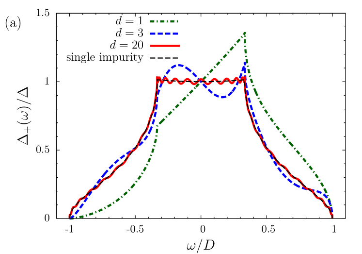
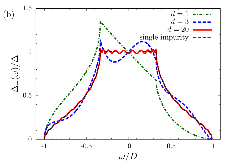
Figure 5: (Color online) Hybridization functions normalized to the Anderson width $\Delta$ for the even (a) and odd (b) channel for various impurity-impurity distances $d=|\underline{d}|$ and momentum independent hybridization matrix element, $|V_{\underline{k}}|^{2}\equiv|V|^{2}$. For comparison the single impurity hybridization function is also shown, which is nothing but the rescaled density of states of the noninteracting band electrons.

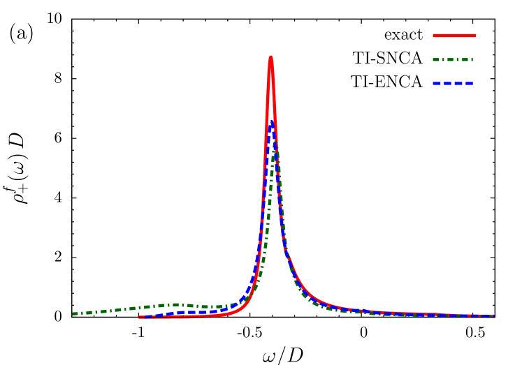
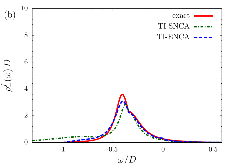
Figure 6: (Color online) Exact spectral functions of the resonant level with $\epsilon^{f}=-0.4D$ [see Eq. (27)] in the even (a) and odd (b) channel for distance $d=1$ compared to the two-impurity (TI-) SNCA and ENCA results.

The exact curves for $U=0$, $\epsilon^{f}=-0.4D$ and distance $d=|\underline{d}|=1$ are compared with the results of the two-impurity SNCA and two-impurity ENCA calculations in Fig. 6. Although the overall features of all curves show rough agreement, the two approximations perform differently in detail. Both capture the van-Hove singularity on the right flank of the resonance at $\omega/D=-\frac{1}{3}$, but the two-impurity ENCA comes closer to the exact solution than two-impurity SNCA. The position and height of the maximum is also captured better by the two-impurity ENCA. Additionally, the two-impurity SNCA produces some unphysical weight in the left flank of the peak at $\omega/D\approx 0.75$.

As mentioned in the previous section such deficiencies had to be expected. They turn out, however, to be less pronounced as one might have feared, so that even in this most critical case of uncorrelated impurities a reasonable result is produced by the two-impurity ENCA. As in the single impurity case, the performance should even increase when correlations become important for $U>0$.

We now turn to the Kondo regime with $U\gtrsim-2\epsilon^{f}>\Delta$. The hybridization $\hat{V}$ tends to produce separate Kondo effects at each impurity controlled by the diagonal elements of the hybridization functions $\Delta_{jj}(\omega)$, but additionally, the non-diagonal element of the hybridization, $\Delta_{lj}(\omega)$ (with $l\neq j$), will produce a RKKY-interaction between the local magnetic moments on the impurities. In order to benchmark the approximations we neglected the latter for the moment and set $\Delta_{lj}(\omega)=0$ for $l\neq j$.

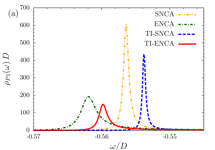
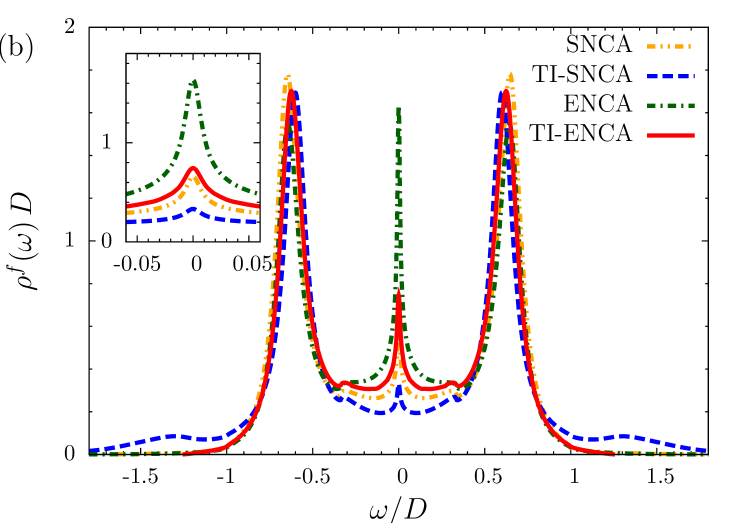
Figure 7: (Color online) (a) Threshold behavior of the different SIAM and the decoupled TIAM approximations deduced from the ionic propagator for one electron per site and for $\epsilon^{f}=-\frac{D}{2}$, $U=D$, $T=0.003D$, and $\Delta=0.1D$. For the SIAM $\rho_{P1}(\omega)=-\frac{1}{\pi}$Im$[P_{\sigma,\sigma}(\omega+i\delta)]$ and for the TIAM as $\rho_{P1}(\omega)=-\frac{1}{\pi}$Im$[P_{\sigma\sigma^{\prime},\sigma\sigma^{\prime}}(\omega/2+i\delta)]$. (b) Full one-particle spectral functions of the different approximations for the same parameters as in (a). The inset shows a close-up of the region around the Fermi level.

Calculations for the Kondo regime are presented in Figs. 7(a) and 7(b). Care has to be taken to facilitate a comparison with the results of single-ion SNCA- and ENCA-solvers, which are shown in these figures, too. Since our two-impurity SNCA and ENCA calculations treat the two-impurity systems, though not coupled, as a whole, the groundstate energy and threshold energies for local excitations should have twice their single-ion value, and the single-particle spectral functions are normalized to two. Hence the energies and curves are correspondingly scaled with a factor of two to be comparable.

Figure 7(a) shows the spectrum of the ionic propagator in the energy region around the ionic threshold for singly occupied impurities, i.e. $\rho_{P1}(\omega)=-\frac{1}{\pi}$Im$[P_{\sigma,\sigma}(\omega+i\delta)]$ for the SIAM and $\rho_{P1}(\omega)=-\frac{1}{\pi}$Im$[P_{\sigma\sigma^{\prime},\sigma\sigma^{\prime}}(\omega/2+i\delta)]$ for the two-impurity model. As is well knownGrewe et al. (2008); *schmittSus09 the ENCA performs considerably better than the SNCA since, for instance, it produces a more accurate, i.e. larger, Kondo temperature $T_{\mathrm{K}}$. $T_{\mathrm{K}}$ can be estimated as the difference between the threshold, i.e. the position of the maximum in $\rho_{P1}$, and the single-particle energy, $T_{\mathrm{K}}\sim E_{\mathrm{threshold}}-\epsilon^{f}$. The same apparently holds when comparing of the two-impurity SNCA and two-impurity ENCA approximation. The two-impurity ENCA even seems to exceed the single-impurity SNCA and comes near to the quality of the single-impurity ENCA, at least for the typical parameter values shown.

A similar conclusion can be drawn from the one-particle spectral functions of Eq. (13) shown in Fig. 7(b). They exhibit the typical three-peak structure with a Kondo-resonance near the Fermi-level and large spectral weight at the so-called Hubbard peaks which originate from the ionic one-particle energies $\epsilon^{f}$ and $\epsilon^{f}+U$. While the high-energy features of the SIAM and TIAM solutions are in good agreement, the low-energy Kondo resonances of the TIAM are less pronounced. All curves are calculated with the same absolute temperature $T=0.0003D$ which implies different relative temperatures to the corresponding Kondo scale of each approximation. The TIAM solutions produce a slightly smaller Kondo scale and consequently the peaks are not as high, which confirms the conclusions drawn from the ionic propagators.

The good qualitative and mostly also quantitative agreement of the calculations support our confidence in the validity of the results presented for coupled impurities in the next section.

V Results for coupled impurities

The physics of a fully coupled cluster of two impurities can become amazingly rich when all possible sources of interactions are taken into account. We therefore restrict ourselves to a few important cases, which we first will consider separately in order to clarify basic physical effects.

In general, the hybridization part of the Hamiltonian will not only induce the tendency towards a local Kondo-screening of moments considered in the previous section, but will also induce an additional effective RKKY-exchange interaction with the asymptotic form in leading order perturbation theoryFazekas (1999)

$$J_{\mathrm{RKKY}} \propto-V^{4}\frac{\sin(2k_{\mathrm{F}}d)+2k_{\mathrm{F}}d\cos(2k_{\mathrm{F}}d)}{\left(2k_{\mathrm{F}}d\right)^{4}},$$ (30)

where $k_{\mathrm{F}}$ is the Fermi wave vector along the distance $d\gg 1$ between the impurities (lattice constant $a=1$). The RKKY-interaction according to Eq. (30) oscillates with distance and can induce a ferromagnetic or antiferromagnetic coupling.

V.1 Isolated two-impurity cluster

It is instructive to consider, what physics already is included without hybridization $\hat{V}$ to the bandstates. For this purpose one can inspect the exact solution of the eigenvalue problem for the isolated cluster $(\hat{V}=0)$ in the presence of interactions which amounts to setting all hybridization functions to zero, $\Delta_{jl}(\omega)=0$. We include a direct magnetic exchange term and also allow for a direct single-electron transfer,

$$\hat{W}^{f}= \sum_{\sigma}t({\hat{f}}^{\dagger}_{1\sigma}\hat{f}^{\phantom{\dagger}}_{2\sigma}+h.c.)-J\underline{\hat{S}}^{f}_{1}\underline{\hat{S}}^{f}_{2}.$$ (31)

Since the exchange interaction has no effect on the one-particle sector of the cluster, the one-particle eigenstates correspond to the (anti-)symmetrized operators given in Eq. (23) with eigenenergies

$$E^{(1)}_{\pm}=\epsilon^{f}_{\pm}=\epsilon^{f}\pm t.$$ (32)

The two-particle sector contains six states, three of which belong to a degenerate triplet with one electron on each of the sites. For these states spin-conserving hopping is ineffective due to the Pauli-principle, which leads to:

$$|S=1,m=\sigma\rangle=|\sigma\rangle_{1}|\sigma\rangle_{2},$$ (33)

$$|S=1,m=0\rangle=\frac{1}{\sqrt{2}}\Big{(}|\uparrow\rangle_{1}|\downarrow\rangle_{2}+|\downarrow\rangle_{1}|\uparrow\rangle_{2}\Big{)}$$

with eigenenergies

$$E_{T}^{(2)}=2\epsilon^{f}-\frac{J}{4}.$$

The three remaining singlets in the two-particle subspace are

$$|S=0,m=0\rangle_{0}=\frac{1}{\sqrt{2}}\Big{(}|\uparrow,\downarrow\rangle_{1}|0\rangle_{2}-|0\rangle_{1}|\uparrow,\downarrow\rangle_{2}\Big{)}$$ (34)

$$E^{(2)}_{S_{0}}=2\epsilon^{f}+U,$$

and

$$|S=0,m=0\rangle_{\pm}=\frac{1}{N_{\pm}}\Bigg{[}\frac{1}{\sqrt{2}}\Big{(}|\uparrow\rangle_{1}|\downarrow\rangle_{2}-|\downarrow\rangle_{1}|\uparrow\rangle_{2}\Big{)}$$

$$\phantom{MMMMMMMM}+a_{\pm}\Big{(}|\uparrow,\downarrow\rangle_{1}|0\rangle_{2}+|0\rangle_{1}|\uparrow,\downarrow\rangle_{2}\Big{)}\Bigg{]}$$

$$E^{(2)}_{S_{\pm}}=2\epsilon^{f}+\frac{3J}{4}-a_{\pm}$$ (35)

where

$$a_{\pm}= \frac{3J}{8}-\frac{U}{2}\Big{(}1\pm\sqrt{1+\frac{16t^{2}}{U^{2}}+\frac{9J^{2}}{16U^{2}}-\frac{3J}{2U}}\Big{)},$$

$$N_{\pm}= \sqrt{1+2\frac{t^{2}}{a_{\pm}^{2}}}.$$

In order to understand the result it is useful to realize that for the polar state $|S=0,m=0\rangle_{0}$ direct transfer is irrelevant due to orbital antisymmetry. The effect of direct hopping on the remaining two singlets, as well as the influence of direct exchange $J$ are most clearly seen in the limiting case where $U$ exceeds $t$ and $J$, i.e. $U\gg|t|,|J|$, where one finds

$$E^{(2)}_{S_{+}}\approx 2\epsilon^{f}+U+\frac{4t^{2}}{U},$$ (36)

$$E^{(2)}_{S_{-}}\approx 2\epsilon^{f}+\frac{3J}{4}-\frac{4t^{2}}{U}.$$ (37)

In this limit the well known competition between the triplet of Eq. (33) and the singlet of Eq. (37) for becoming the ground state is realized. The physics is determined by the exchange splitting of these levels,

$$\Delta E=E^{(2)}_{S_{-}}-E^{(2)}_{T}=J-\frac{4t^{2}}{U}\equiv J+J_{t}.$$ (38)

For larger values of the direct transfer $t$ the level-splitting becomes increasingly important and renders a discussion based exclusively on an effective exchange interaction impossible.

States with three or four electrons in the cluster have higher energies through additional contributions of $U$. They can be deduced from the above results by particle-hole transformation.

V.2 Direct exchange coupling

For the following numerical study we will set $t=0$ but consider a direct coupling $J$. We also include a finite diagonal hybridization but still ignore the non-diagonal hybridization functions producing the RKKY interaction, i.e. $\Delta_{12}(\omega)=0$. Therefore, we choose a direct two-impurity interaction Hamiltonian [see Eq. (2)]

$$\hat{W}^{f}= -J\underline{\hat{S}}^{f}_{1}\underline{\hat{S}}^{f}_{2}.$$ (39)

Then, the typical competition between the single-ion Kondo effects and the fixed nonlocal exchange $J$ results. The Kondo coupling between each impurity spin and the conduction electrons is governed by the antiferromagnetic exchange

$$J_{\mathrm{Kondo}}=-\frac{2U\Delta}{\epsilon^{f}(\epsilon^{f}+U)}>0$$ (40)

leading to a characteristic energy scale

$$T_{\mathrm{K}}=\alpha\sqrt{J_{\mathrm{Kondo}}}\exp\big{(}-\pi/J_{\mathrm{Kondo}}\big{)}$$ (41)

with $\alpha\approx 2\pi\min\{U,D\}$.

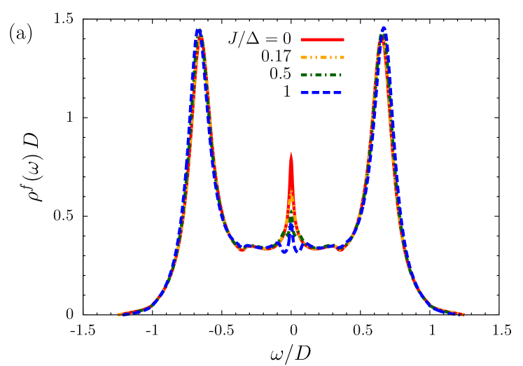
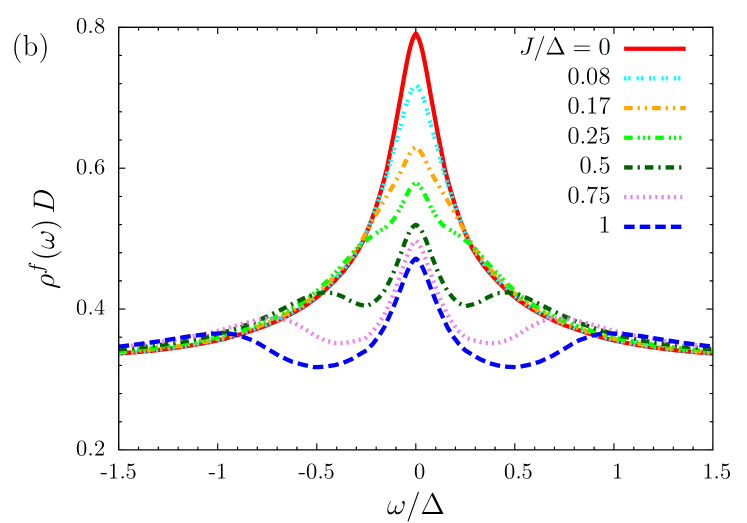
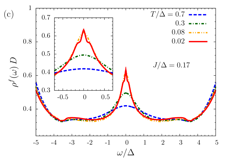
Figure 8: (Color online) Spectral function for $\epsilon^{f}=-\frac{D}{2}$, $U=D$, $\Delta=0.1D$ with direct ferromagnetic coupling $J>0$: (a) Fixed temperature $T=0.004D=0.04\Delta$ and various values of the coupling. (b) Magnification of the region around the Fermi-energy. (c) The spectral function near the Fermi level for fixed coupling $J=0.017D=0.17\Delta$ and various temperatures. Notice, that while in panel (a) the energy is measured in units of the half-bandwidth $D$, panels (b) and (c) use the Anderson width $\Delta$.

One-particle spectral functions calculated with the two-impurity ENCA-solver are shown in Fig. 8 for various values of a ferromagnetic direct coupling ($J>0$) and temperatures. The overall form of the spectral function and the high-energy features are essentially unchanged under the inclusion of $J$. However, pronounced changes occur in the low-energy region around the Fermi energy $\omega=0$, which at $J=0$ and small $T\lesssim T_{\mathrm{K}}$ exhibits the well-known many-body resonance of the single-ion Kondo effect.

For very large direct exchange coupling $J>0$ the two impurity spins are aligned parallel and nearly act as one rigid spin with $S=1$. This corresponds to the triplet state in the isolated cluster which experiences a modified two-stage nonlocal Kondo screening with a reduced characteristic energy scale $T_{\mathrm{K}}^{\mathrm{(2imp)}}<T_{\mathrm{K}}$.Silva et al. (1996) This leads to the formation of a narrower and less saturated Kondo resonance at $\omega=0$, clearly visible in Fig. 8(b) and is similar to what happens in multi-orbital SIAM.Kubo and Hirashima (1999); *pruschkeTwoBandHMNRG05; *nevidomskyyHundJKondo09

At excitation energies of the order of the exchange coupling, $\omega\approx\pm J$, one probes a domain dominated by correlations typical for the single-ion Kondo effect. The weaker nonlocal correlations of the low-energy regime are then broken. The two impurities appear as essentially uncoupled and behave like isolated single impurities. In the spectral functions this is indicated by the humps visible for small $J$ which develop into side-maxima at larger $J$ which are located the energies $\omega\approx\pm J$. For energies larger than $|\omega|>J$ the $J=0$ spectral function is approached. This is in accord with the finding, that the characteristic high-energy scale of this model is essentially given by the single-impurity Kondo scale.Zhu and Zhu (2011)

This is also reflected in the temperature dependency as shown in Fig. 8(c). The many-body resonance at first forms like in a SIAM, and only for low temperatures $T\lesssim J$ the narrowing near the Fermi level sets in and causes the above mentioned humps or maxima.

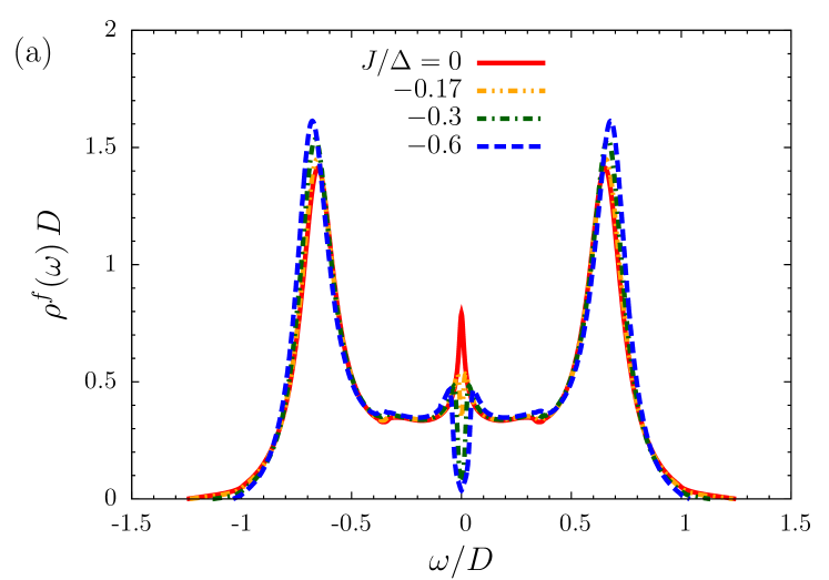
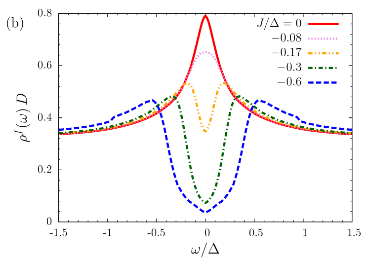
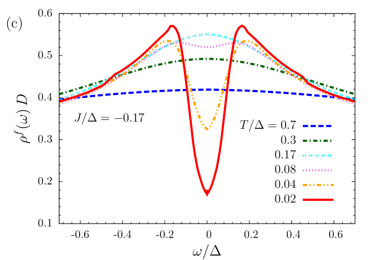
Figure 9: (Color online) (a) Spectral functions for various antiferromagnetic direct exchange couplings $J<0$ and fixed temperature $T=0.04\Delta$. Panel (b) shows a magnification of the low energy region. (c) The spectral function around the Fermi level for fixed coupling $J=-0.17\Delta$ and various temperatures. Notice, that while in panel (a) the energy is measured in units of the half-bandwidth $D$, panels (b) and (c) use the Anderson width $\Delta$. Other parameters are as in Fig. 8.

We now turn to the case of an antiferromagnetic direct coupling ($J<0$) where the nature of the physical scenario for low lying states changes qualitatively. Now a real competition takes place between local singlet formation via the Kondo-effect and nonlocal singlet binding in the molecular two-electron state. The single-ion Kondo effect present at small $J$ is suppressed with increasing negative values of $J$. This is clearly borne out by the spectral functions of Fig. 9, which exhibit a very rapid depletion of the spectral function near the Fermi energy with $|J|$.

The formation of a gap around $\omega=0$ then implies that the low lying molecular singlet does effectively not interact with the band states. However, side peaks at the edges of the gap can be observed at energies $\omega=\pm J$. These are indicative for the fact that the excited molecular triplet experiences a kind of virtual Kondo effect.Paaske et al. (2006)

This interpretation is supported by the temperature dependence of the curves depicted in Fig. 9(c) for a fixed value of $J=-0.17\Delta$. In the same way as the pseudogap around $\omega=0$ forms for temperatures lower than $|J|$, the side peaks emerge and increase in height.

V.3 Direct single-particle hopping

We now neglect the direct magnetic exchange, but introduce a direct single-particle hopping, i.e.

$$\hat{W}^{f}= t\sum_{\sigma}({\hat{f}}^{\dagger}_{1\sigma}\hat{f}^{\phantom{\dagger}}_{2\sigma}+h.c.).$$ (42)

We still ignore the non-diagonal hybridization

$$\Delta_{12}(\omega) =0.$$ (43)

Based on the discussion of the isolated two-impurity cluster in Sect. V.1 we can expect a twofold source for modifications of a pure single-ion Kondo effect: (1) $t$ gives rise to an effective antiferromagnetic exchange interaction $J_{t}=-\frac{4t^{2}}{U}$, and (2) $t$ splits the ionic one-particle levels $\epsilon^{f}\rightarrow\epsilon^{f}_{\pm}$ and produces a tendency towards even and odd molecular one-particle states. Therefore, the interesting question arises, how the scenario developed for an antiferromagnetic direct exchange interaction will be altered by the impending effect of even-odd splitting.

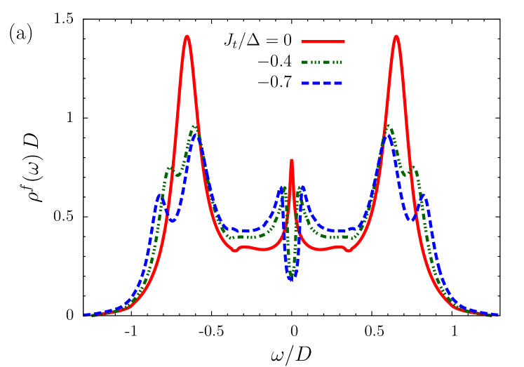
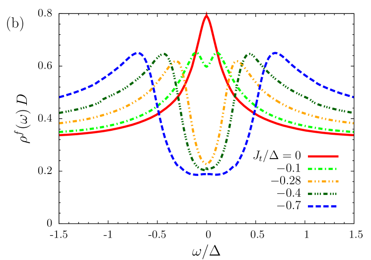
Figure 10: (Color online) (a) Spectral functions at a fixed temperature $T=0.04\Delta$ for various values of the direct single-particle hopping $t$. To reveal its physical influence more clearly the effective antiferromagnetic exchange $J_{t}=-\frac{4t^{2}}{U}$ is given instead of the bare hopping $t$. For example, $J_{t}=-0.4\Delta$ corresponds to $t=0.1D$ and $J_{t}=-0.7\Delta$ corresponds to $t=0.13D$. Panel (b) shows a magnification of the low energy region (energy is measured in units of the Anderson width $\Delta$). Other parameters are as in Fig. 8.

Figure 10 shows the spectral function for various values of $t$. One recognizes the expected opening of the pseudogap around the Fermi level $\omega=0$ with increasing absolute value of $J_{t}$ [see panel (b)].

The hopping induces changes of the spectral function at all energies [see 10(a)], which is in contrast to the case of a direct coupling where only the low-energy region was affected. Particularly, and in accord with our expectations, the ionic Hubbard resonances near $\omega=\epsilon^{f}$ and $\omega=2\epsilon^{f}+U$ are split by the hopping. The separation of the peak maxima is roughly given by $2t$ which is in accord with the simple reasoning from the isolated two-impurity model, see Eq. (32). This reflects a tendency, which has been outlined beforeGrewe (2005), namely that features of the unperturbed structures of the one-particle states leave their traces in the quasiparticle bandstructure.

In the low-energy region, hopping produces a gap similar to the case of a direct exchange coupling [see Figs. 9(b) and 10(b)]. However, whereas the gap is not as pronounced as in Fig. 9(b), the side peaks at the edge of the gap are considerably higher.

The question arises whether the splitting is due to a suppression of the Kondo effect as in the case of a direct antiferromagnetic $J$. It can be addressed by decomposing the spectral function into even and odd parity parts as would be produced by the operators ${\hat{f}}^{\dagger}_{\pm\sigma}$ of Eq. (23). This is shown in Fig. 11 for $t=0.1D$, i.e. $J_{t}=-0.4\Delta$. All the peaks in the spectral function can clearly be attributed to (mostly) one parity channel. In particular, the quasiparticle Kondo resonance is partitioned into an odd contribution for negative energies and an even contribution for positive energies.

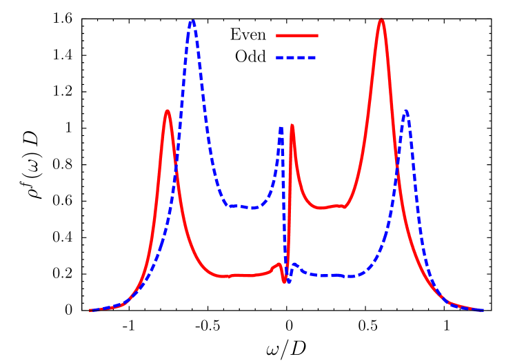
Figure 11: (Color online) Spectral function of Fig. 10(a) for $J_{t}/\Delta=-0.4$ decomposed onto even and odd contributions.

This suggests that the splitting is not exclusively due to a suppressed Kondo effect, but is mainly a single-particle even-odd splitting of the quasiparticle excitations. The side peaks then indicate the local preformation of quasiparticle bands, with the odd states associated with the bonding region at $k=0$ and the even states with the anti-bonding region at $k=\pm\pi$.

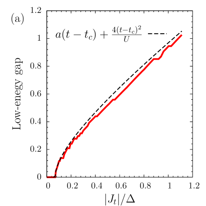
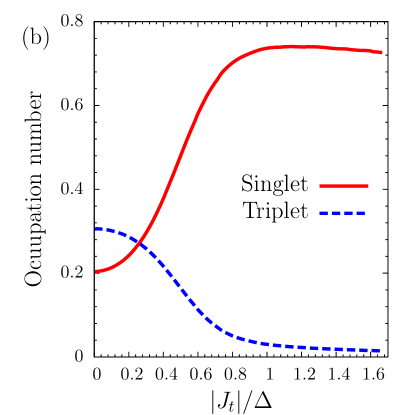
Figure 12: (Color online) (a) Low-energy gap as function of $|J_{t}|$. The parameters for the dashed fit are $t_{c}=0.05\Delta$ and $a=2.16\Delta$ (b) Occupation numbers of the singlet and triplet states in the two-particle sector as function of the (negative) effective antiferromagnetic exchange $J_{t}$. All other parameters are as in Fig. 10.

We show the width of the central low-energy pseudogap as function of the effective exchange $|J_{t}|=\frac{4t^{2}}{U}$ in Fig. 12(a). The gap first opens at a finite value $t_{c}$ for the hopping. For smaller values of $J_{t}$ the splitting behaves like a square root indicating an opening of the gap which is linear in $t$. At larger $t$ the gap is dominated by the impact of the quadratic $t$-dependence of the exchange coupling and thus goes linear in $|J_{t}|$. Indeed a fit with a function $a(t-t_{c})+4\frac{(t-t_{c})^{2}}{U}$ reproduces the gap quite well.

The molecular triplet and singlet states are separated in energy roughly by $|J_{t}|$ [see Eq. (38)]. At large $t$ the singlet becomes lower in energy that the triplet. This can be directly observed in Fig. 12(b), where the occupation numbers of these molecular states are shown as function of $|J_{t}|$. For small $|J_{t}|$ the occupation numbers are roughly equal and mixed at a nearly constant ratio. With increasing coupling, the singlet occupation rises steeply, accompanied by a corresponding fast depletion of the triplet states. The large-$|J_{t}|$ regime thus reproduces the behavior already known from a direct antiferromagnetic exchange.

V.4 Non-diagonal hybridization and RKKY exchange

It is left now to clarify the role played by the non-diagonal hybridization. We set the direct parameters $t$ and $J$ to zero and include the full hybridization function of Eq. (20), which allows for a coherent hybridization of the cluster states with the conduction band. The non-diagonal component for distance $\underline{d}=\underline{R}_{2}-\underline{R}_{1}$ reads

$$\Delta_{12}(\omega)= \frac{1}{N}\sum_{\underline{k}}V^{2}\cos(\underline{k}\underline{d})\pi\delta(\omega-\epsilon^{c}_{\underline{k}}).$$ (44)

The process of non-diagonal hybridization is qualitatively different from a direct hopping $t$ as considered before. As a consequence of the intermediate propagation through the band, a nontrivial dependence on the excitation energy $\omega$ results. The hybridization function exhibits an increasingly oscillatory behavior with growing distance between the impurities while the absolute height decreases as shown in Fig. 13.

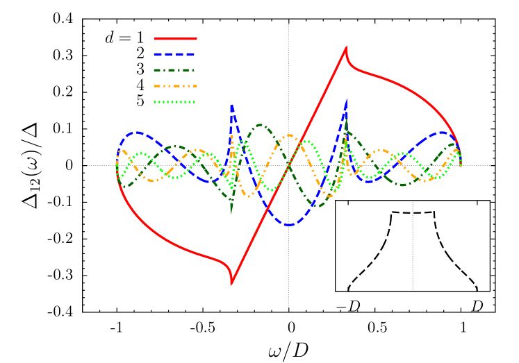
Figure 13: (Color online) Non-diagonal hybridization function of Eq. (44) for various distances as indicated. The inset sketches the three-dimensional free density of states of the conduction electrons.

The following effects are expected as consequences of diagonal and this non-diagonal hybridization: (1) the RKKY-exchange interaction between the two impurity spins is induced, which favors ferro- or antiferromagnetic alignment depending on the distance. (2) Kondo screening-clouds (see, for example, Ref. Borda, 2007; *buesserKondoCloud10; *mitchellKondoCloud11; *prueserKondo11) for singly occupied impurities are induced in the band. In case the impurities are spatially not well separated and the individual Kondo-clouds penetrate each other, this then involves considerable nonlocal coherence. (3) A tendency toward the stabilization of even and odd parts of the molecular single-electron orbitals might appear, as the result of an induced (indirect) transfer via the band states.

Thus, we do not expect a simple realization of the Doniach-scenario of competing local and antiferromagnetic correlations, which would either lead to a Fermi liquid with quenched spins (and some short-ranged antiferromagnetic correlations) or to antiferromagnetic order between the impurities.

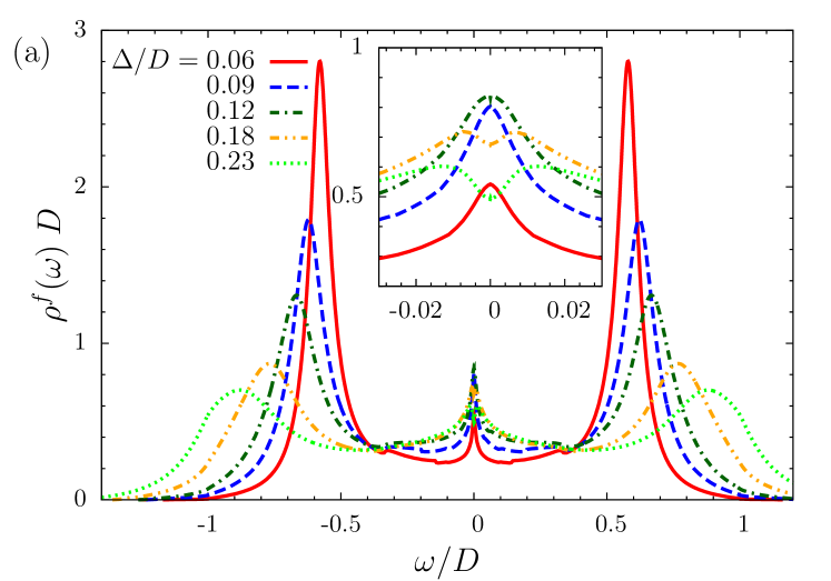
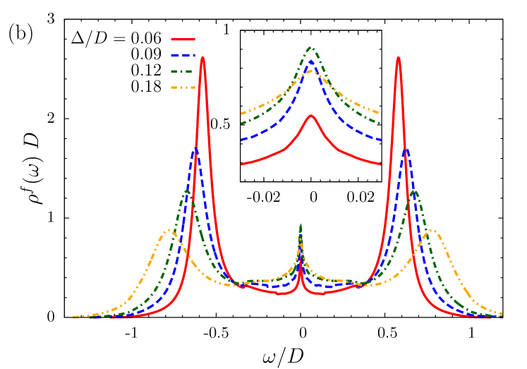
Figure 14: (Color online) Impurity spectral functions with diagonal and non-diagonal hybridization functions for two distances (a) $|\underline{d}|=1$ and (b) $|\underline{d}|=2$ for various Anderson widths as indicated. The inset shows a close-up of the low energy region. Other parameters are: $\epsilon^{f}=-\frac{D}{2}$, $U=D$, $T=0.004D$ and $J=t=0$.

In Figure 14 the one-particle impurity spectral functions for two different impurity distances along the same principal direction of a three-dimensional simple-cubic lattice are shown for various values of the hybridization strength $\Delta$. These cases can loosely be associated with situations already studied above. Our choice of parameters places the nearest-neighbor $d=1$ case into a regime of antiferromagnetic exchange, $J_{\mathrm{RKKY}}<0$, whereas at $d=2$ the impurities should experience a ferromagnetic $J_{\mathrm{RKKY}}>0$.

The spectra greatly change with increasing hybridization. The Hubbard peaks are broadened and are moved to larger energies, as it is expected. These high-energy features are mainly determined by the diagonal part of the hybridization and are insensitive to the distance between the impurities, thus the figures of panel (a) and (b) are very similar at large $|\omega|$. Increasing $\Delta$ first implies a larger absolute value of $J_{\mathrm{RKKY}}<0$ for $d=1$. Consequently, a pseudogap forms at the Fermi level for $\Delta\gtrsim 0.15D$ as visible in the inset of Fig. 14(a). The reason for the gap being not visible at smaller $\Delta$ is the finite temperature of $T=0.004D$ used in the calculation.

For distance $d=2$ the larger ferromagnetic $J_{\mathrm{RKKY}}$ should lead to a narrowing of the many-body resonance with side-peaks, but this is not clearly observed in Fig. 14(b). On the other hand, the local single-impurity Kondo scale is also enhanced with increasing $\Delta$ [see Eq. 41], leading to an increase in the overall spectral weight of the Kondo resonance at the Fermi level. (This is also observed in the case of the antiferromagnetic $d=1$ situation.) The signatures of indirect ferromagnetic exchange are by far not as clear as in the case studied in a previous section with direct exchange. For one, they are strongly competing with the increasing single-ion Kondo effect and for another, the dynamic non-diagonal exchange does not act in the same simple way as an static exchange constant. Therefore, the Doniach scenario seems to be too oversimplifying.

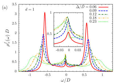
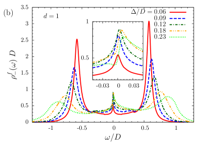
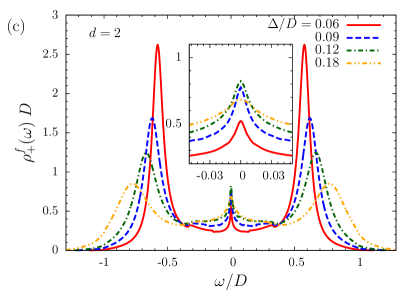
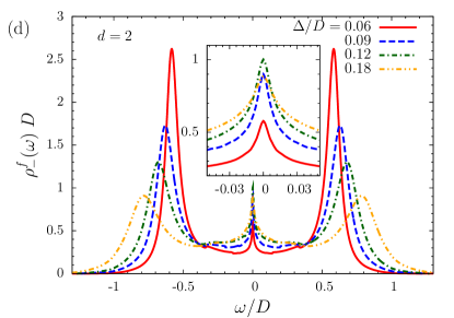
Figure 15: (Color online) Impurity spectral functions decomposed into even [(a) and (c)] and odd [(b) and (d)] contributions for distance $|\underline{d}|=1$ [(a) and (b)] and $|\underline{d}|=2$ [(c) and (d)] for various Anderson widths. The inset shows a close-up of the low energy region. All other parameters are as in Fig. 14.

The influence of molecular correlations favoring even and odd one-particle states via an induced effective transfer can again be derived from a decomposition of the spectra in the even and odd parity components. These are shown in Fig. 15 for the same parameters as in Fig. 14. It is obvious, that the indirect hopping is much less effective in producing even-odd splitting when compared to the direct hopping of the previous section. The even and odd spectral functions are very similar to each other and only for the small distance $d=1$ moderate asymmetries occur. The splitting is noticeable, though not nearly as strong as in Fig. 11. But interestingly, the splitting of the low-energy quasiparticle peak at the Fermi level is much more pronounced than the imbalance of the high-energy Hubbard peaks. This supports the idea that nonlocal correlations cause the coherence in the low-energy region where the Kondo effect develops. They also lead to pseudogap formation and in consequence to the notion of a impending quasiparticle bandstructure, a viewpoint already adopted above.

For $d=2$ such an effect is barely visible and an asymmetry can not be observed in the spectral functions. The odd channel has a slightly larger spectral weight in the many-body resonance around the Fermi level as compared to the even spectra.

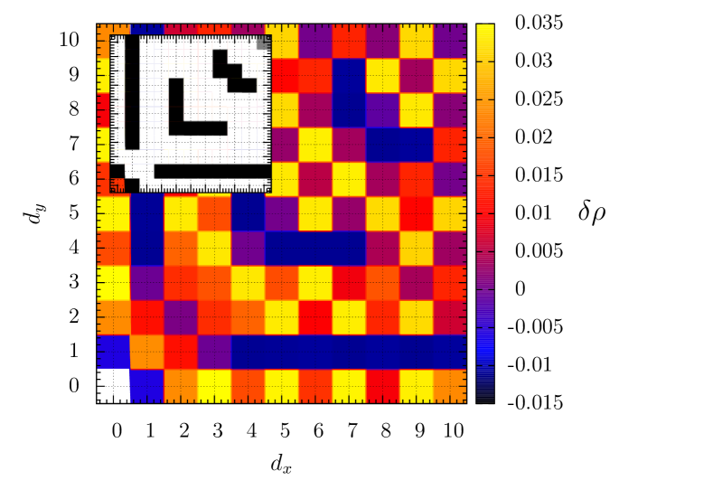
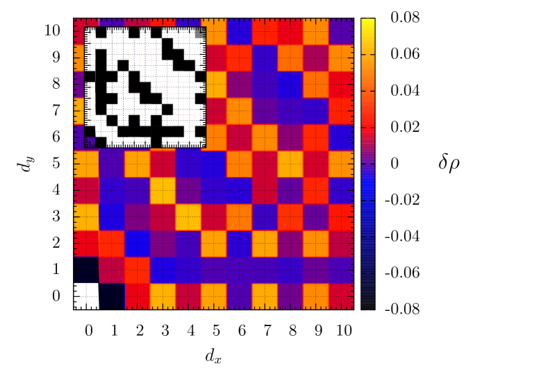
Figure 16: Height of the two-impurity spectral function at $\omega=0$ relative to its value without the second impurity [see Eq. (45)]. (a) $\Delta=0.11D$ (b) $\Delta=0.16D$. One impurity is located at the origin, while the other at the distance vector $\underline{d}=d_{x}\underline{e}_{x}+d_{y}\underline{e}_{y}$. The insets show the sign of this quantity, where black denotes $\Delta\rho<0$ and white $\Delta\rho>0$. All other parameters are as in Fig. 14.

The investigation of the effective transfer- and exchange can easily be extended to other relative positions of the two impurities in a cubic lattice. As one might expect, an oscillation of physical quantities which can be associated with ferromagnetic or antiferromagnetic tendencies is found with varying distance. One example of such an oscillating quantity is the height of the many-body resonance right at the Fermi level in comparison to its value without the second impurity, i.e.

$$\delta\rho=\rho(\omega=0)-\rho_{|\underline{d}|=\infty}(\omega=0).$$ (45)

We present this quantity in Fig. 16 for two different hybridization strengths as a function of the two-impurity distance $\underline{d}=d_{x}\underline{e}_{x}+d_{y}\underline{e}_{y}$ in a two-dimensional plane, where one impurity is always located in the origin. Red and yellow colors imply a larger height of the two-impurity spectral function than in a SIAM, while black and blue colors indicate a suppression of $\rho(\omega=0)$.

Regions with enhancement and suppression of the many-body resonance can be clearly identified. While a suppression can easily be explained by the antiferromagnetic exchange coupling, the reason for an enhancement is not as clear. We attribute it to the effect of the dynamic non-diagonal hybridization, producing a constructive interference and an effectively larger total hybridization. However, the spatial pattern is not simply determined by the Manhattan distance, i.e. the number of elementary hoppings between the two impurities. It appears, that more complicated interferences of single-particle and interaction effects obviously play a role. For very large distances these short-distance effects should be irrelevant and an asymptotic form like Eq. (30) is expected.

VI Conclusion

In this work we have presented a novel two-impurity solver which is based on direct perturbation theory with respect to the hybridization. It is capable of treating any kind of direct interaction of the two-impurities as well as the dynamical indirect coupling via the conduction band.

Including separately different couplings of the two impurities we carefully investigated the role played by each and the resulting physical mechanisms. In situations, where the impurities are not coupled via the conduction electrons but only directly, we found that a ferromagnetic exchange leads to a narrowing of the many-body resonance which is characteristic of a higher-spin Kondo effect.

For antiferromagnetic coupling, the inter-impurity singlet formation competes with two separate local Kondo effects. This leads to the suppression of the Kondo effect due to singlet-triplet splitting at small enough temperature which is clearly signalled by a pseudo-gap opening in the many-body resonance at the Fermi level.

Interestingly, such a pseudo-gap is also induced without direct exchange coupling but instead including a direct single-electron hopping between the impurities. This produces a splitting of bonding and anti-bonding two-impurity orbitals, i.e. of even and odd parity components of the spectral function. Additionally, an effective antiferromagnetic exchange is generated by a finite hopping. This also supports the formation of a gap in the many-body resonance which, however, is accompanied by sharp side-peaks of the even and odd excitations.

In the generic scenario without direct interactions between the impurities but with couplings generated indirectly via the conduction electrons the situation is not as clear. Signatures of the induced RKKY interaction are observable in form of oscillatory behavior with varying distance between the impurities. It seems that the induced magnetic exchange interactions are the dominant source of competition with isolated Kondo effects. Molecular correlations and splitting of even and odd parity channels induced by an effective single-particle hopping between the impurities are only observable for smallest distances. Even though the total size of these effects is rather small, the low-energy many-body physics seems to be very sensitive to this kind of perturbation.

Although the well known Doniach-scenario captures essential aspects of the physics involved, we are led to the conclusion that the coupled two-site cluster exhibits a much richer physical behavior, in particular at small impurity distances. For this reason the dynamical non-diagonal hybridization function needs to taken into account.

The ability of the solver to work with arbitrary two-impurity distances and arbitrary hybridization functions allows for utilization in a nonlocal extension of dynamical mean-field theory.Pruschke et al. (1995); *georges:dmft96 We propose such a scheme where two-site correlations are included in a separate publicationJabben et al. (2012) and the results with the two-impurity ENCA as impurity solver are very promising.