A new method for deriving incidence rates from prevalence data and its application to dementia in Germany

Abstract

This paper descibes a new method for deriving incidence rates of a chronic disease from prevalence data. It is based on a new ordinary differential equation, which relates the change in the age-specific prevalence to the age-specific incidence and mortality rates. The method allows the extraction of longtudinal information from cross-sectional studies. Applicability of the method is tested in the prevalence of dementia in Germany. The derived age-specific incidence is in good agreement with published values.

Keywords: Chronic diseases; Dementia; Incidence; Prevalence; Mortality; Compartment model; Cubic spline; Ordinary differential equation.

1 Introduction

Basic epidemiological characteristics of a disease are the prevalence, the proportion of diseased persons in the population, and the incidence, which focusses on the number of new cases. Both characteristics are fundamentally different: the first measures the actual presence of the disease, the second refers to the new cases. Typically, prevalence and incidence of a disease are surveyed in observational studies. The prevalence can easily be assessed in cross-sectional studies: The study population is interviewed or examined with respect to the disease. The classical approach to measure incidence is the cohort study, which is somewhat more complex. A certain group of patients is examined whether the disease exists at the start of the study. The healthy individuals of the group will be examined at least once more at a later point in time, to find out whether the disease occured in the meanwhile. Since at least one follow-up investigation must take place, a cohort study mostly is much more complex and expensive than a cross-sectional study. Particular difficulties arise due the fact that participants get lost after the baseline examination (loss to follow-up).

For some questions, the incidence of a disease is more important than knowing the number of those who are already ill. Many of the questions in health services research, such as the allocation of resources need information about the number of expected patients. Within epidemiology, there are several attempts to derive incidences from prevalence data. A simple, popular example may illustrate this. Consider a closed population of size $N$; this means there is no migration and the numbers of births and deaths are exactly the same for the considered period of length $\Delta t>0$. Let $C$ denote the number of persons in the population who suffer from a chronic disease ($C$ stands for cases). Assuming that the number of diseased persons for the time period is constant, it follows that the number of new cases is just equal to the number of patients who die. Hence, it holds

$$\left(N-C\right)\cdot i\cdot\Delta t=C\cdot m_{1}\cdot\Delta t,$$

where $i$ is the incidence rate and $m_{1}$ is the mortality of the diseased. By defining the (overall) prevalence $p:=\tfrac{C}{N},$ the term $\tfrac{C}{N-C}$ can be expressed as $\tfrac{C}{N-C}=\tfrac{p}{1-p}$, which is called prevalence odds. Since the inverse of the mortality $m_{1}$ is the mean duration $d$ of the disease, it follows:

$$\frac{p}{1-p}=i\cdot d.$$

This corresponds to the often found statement that the prevalence odds equals the product of incidence and disease duration (see for example (Szklo and Nieto, 2007)). For rare diseases ($1-p\approx 1$) this reads as: prevalence equals the product of incidence and duration.

Beside this simple example, a number of more complex approaches exist to estimate the incidence from prevalence data. The article by Langohr (1999) gives an overview. This work reports about a new method, which is based on a simple compartment model and uses an ordinary differential equation (ODE) to express transitions between the compartments. Compartment models in epidemiology go back at least until the early 1990s (see for example (Keiding et al., 1990)). Murray and Lopez from the Harvard Center for Population and Development Studies describe that they express the transitions between the compartments in terms of ODEs (1994). Without quoting Keiding, they call their model Harvard Incidence-Prevalence Model. Unfortunately, they do not describe their equations. Later they publish another (slightly more complicated) compartment model and present the associated ODEs, (Murray and Lopez, 1996). Our approach builds on the original model of Keiding and a two-dimensional system of ODEs. By analytical transformations this two-dimensional system can be reduced to an one-dimensional ODE. The reduced equation to our knowledge has not yet been published by other groups. We take this equation further to derive the incidence rate from prevalence data. In contrast to the multi-dimensional system of Murray and Lopez, the one-dimensional equation can be solved easily for the incidence.

This paper is organized as follows: Section 2 describes the newly discovered link between the age distributions of the prevalence, incidence and mortality rates. In Section 3 the new method is applied to data of the statutory health insurance (SHI) in Germany. The age distribution of persons with a diagnosis of dementia is used to derive the incidence rates in the associated age groups. Finally, the results are discussed in section 4.

2 The new relation beween incidence, prevalence and mortality

Compartment models are widespread in medicine and other sciences, (Godfrey, 1983). In epidemiology of infectious diseases they play a prominent role with a variety of applications, (Keeling and Rohani, 2007). A simple model for the study of non-infectious diseases is shown in Figure 1. Three states Normal, Disease and Death are considered, plus the transitions between the states, (Keiding, 1991; Murray and Lopez, 1994). In general, the transition rates depend on the calendar time $t$ (sometimes called the period) and the age $a$. Henceforth, only irreversible diseases are considered. The transition from the state Disease to the state Death often depends on the duration $d$ of the disease. The influence of calendar time reflects, for example, the change in mortality or medical progress over decades.

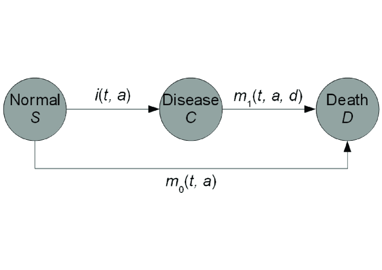
Figure 1: Simple model of a chronic disease with three states. Persons in the state Normal are healthy with respect to the considered disease. In the state Disease they suffer from the disease. The transition rates depend on the calendar time $t,$ on the age $a,$ and in case of the disease-specific mortality $m_{1}$ also on the disease’s duration $d$.

As shown in Figure 1 people in the population get the disease with incidence rate $i$. The mortality rate depends on the state: Non-diseased and diseased persons die with rates $m_{0}$ and $m_{1}$, respectively. Mostly, the rate $m_{1}$ will be higher than the rate of $m_{0}$. For historical reasons, the numbers of individuals in the states Normal and Disease are denoted $S$ (susceptibles) and $C$ (cases), respectively.

Henceforth, we need the following assumptions:

1. The rates $i,m_{0},$ and $m_{1}$ do not depend on calendar time $t$,

2. the mortality rate $m_{1}$ of the diseased does not depend on the duration $d$,

3. the population is closed (i.e. there is no migration),

4. the birth-rates of new-borns with and without the disease are constant over time.

Furthermore, let us assume that the changes in $S$ and $C$ are proportional to the differences of the in- and outflows to and from the compartments:

$$\begin{split}\frac{\mathrm{d}S}{\mathrm{d}a}&=-\left(i(a)+m_{0}(a)\right)\cdot S\\ \frac{\mathrm{d}C}{\mathrm{d}a}&=i(a)\cdot S-m_{1}(a)\cdot C.\\ \end{split}$$ (1)

With these assumptions the central result of this work can be formulated:

Theorem 2.1.

Let mortalities $m,m_{0}\in C^{0}\left(\left[0,\infty\right)\right)$ and $S,C\in C^{1}\left(\left[0,\infty\right)\right)$ with $S(a)+C(a)>0$ for all $a\in\left[0,\infty\right),$ then the age-specific prevalence

$$p=\frac{C}{S+C}$$ (2)

is differentiable in $\left[0,\infty\right)$ and it holds

$$\frac{\mathrm{d}p}{\mathrm{d}a}=(1-p)\cdot\left(i-p\cdot\left(m_{1}-m_{0}\right)\right).$$ (3)

Proof.

This is an easy application of the quotient rule to Eq. (2) using Eq. (1). ∎

Depending on what information is given about the mortalities, the ODE (3) changes its type (see Table 1). Note that the overall mortality $m$ in the population can be expressed as

$$m(a)=(1-p(a))\cdot m_{0}(a)+p(a)\cdot m_{1}(a).$$ (4)

Furthermore, in some cases the relative mortality risk $R(a)=\tfrac{m_{1}(a)}{m_{0}(a)}$ is known.

Table 1: Type of the ODE (3).

Known mortality	Right-hand side	Type of the ODE
$m,m_{0}$	$(1-p)\cdot(i-(m-m_{0}))$	Linear
$m_{0},m_{1}$	$(1-p)\cdot(i-p\cdot(m_{1}-m_{0}))$	Riccati
$m_{0},R$	$(1-p)\cdot(i-p\cdot m_{0}\cdot(R-1))$	Riccati
$m_{1},R$	$(1-p)\cdot(i-p\cdot m_{1}\cdot(1-1/R))$	Riccati
$m,m_{1}$	$(1-p)\cdot\left(i-p\cdot\frac{m_{1}-m}{1-p}\right)$	Abel
$m,R$	$(1-p)\cdot\left(i-m\cdot\left(1-\left(p\cdot\left(R-1\right)+1\right)^{-1}\right)\right)$	Abel

If the ODE is the linear, it can be solved analytically. If it is Riccatian or Abelian, a general solution is not known, (Kamke, 1983). Since the overall mortality $m$ in many populations can be obtained by official life tables; and relative mortality risks $R$ for several diseases often are reported in epidemiological studies, the most important case is when $m$ and $R$ are given. The following section will show an application of this.

Note, that independence from calendar time $t$, zero migration and constant birth rates are crucial for Eq. (1). This can be seen by realizing that the population size $N(a)=S(a)+C(a)$ at age $a$ fulfills the following equation:

$$\frac{\mathrm{d}N}{\mathrm{d}a} =\frac{\mathrm{d}S}{\mathrm{d}a}+\frac{\mathrm{d}C}{\mathrm{d}a}$$

$$=-m_{0}\cdot S-m_{1}\cdot C$$

$$=-N\cdot\left[(1-p)\cdot m_{0}+p\cdot m_{1}\right].$$

Thus, by using Eq. (4) it holds $\tfrac{\mathrm{d}N}{\mathrm{d}a}=-m\cdot N$, which is the defining equation of a stationary population, (Preston and Coale, 1982). These assumptions ensure the population being stationary, (Preston et al., 2001, pp. 53ff).

3 Application to dementia

As already described in the introduction, the most important application is the derivation of the age-specific incidence rate $i(a)$ from the age distribution $p(a)$ of the prevalence of a chronic disease. The usefulness of the method is examined in an example of dementia. Prevalence of dementia in Germany is reported in the work of Ziegler and Doblhammer (2009). Basis for the values published there were claims data from the German statutory health insurance (SHI) in the year 2002. About 90 percent of the whole population in Germany are members of the SHI. A three percent random sample of all of these is used for the analysis. Hence, information of more than 2.3 million people are taken into account.

For each of the persons in the three-percent sample, demographic data (age, gender), the number of doctor visits and hospital stays, both with diagnostic positions in ICD coding, are included. Ziegler and Doblhammer associate the following ICD-10-GM diagnoses with dementia: F00, F01, F02, F03, G30. The resulting prevalences in Germany are reported in Table 2.

Table 2: Prevalence of dementia in members of the German SHI in 2002 Ziegler and Doblhammer (2009)

Age group (in years)	Females (%)	Males (%)
60–64	0.6	0.8
65–69	1.3	1.5
70–74	3.1	3.2
75–79	6.8	5.6
80–84	12.8	10.3
85–89	23.1	17.9
90–94	31.3	24.2

The prevalence data show that dementia is more frequent in women aged $\geq$ 75 years than in men in same age group. Unfortunately Ziegler and Doblhammer have not reported confidence intervals or p-values to decide whether the differences in the age groups are significant. Due to the large sample size this is likely.

For the application of the one-dimensional ODE (3) we need statements about the mortality. Here, we use the general mortality $m$ as surveyed by the Federal Statistical Office of Germany. The relative mortality $R$ of persons with dementia can be found in (Rait et al., 2010): In the first year after the diagnosis of the disease, it is about $3.7$ and in subsequent years about $2.4.$ In this work, the relative mortality is set to be constant at $R(a)=2.4.$

In order to derive the incidence rate $i(a)$ from Eq. (3), the following steps are performed:

1. Derive a spline function $s(a)$ that interpolates the prevalence data.

2. Calculate the derivative $\tfrac{\mathrm{d}s}{\mathrm{d}a}$ and define the function

   $$c=\frac{\mathrm{d}s/\mathrm{d}a}{1-s}.$$

3. The incidence rate $i(a)$ can be expressed by

   $$i(a)=c(a)+m(a)\cdot\left(1-\left(s(a)\cdot\left(R(a)-1\right)+1\right)^{-1}\right).$$

The spline is used to transform the discrete values of the prevalence data into a differentiable function. Here, the uniquely defined cubic spline with natural bounding conditions that interpolates the prevalence data is chosen. It is two times differentiable. Calculations are performed with the statistical software R (The R Foundation for Statistical Computing), version 2.12.0.

Using the prevalence data as shown in Table 2 as input values, following results are obtained with the algorithm described above (Table 3).

Table 3: Age-specific incidence rates for dementia as calculated with the new method.

Age group	Females	Males
(in years)	(per 100 person-years)	(per 100 person-years)
60–64	0.1	0.1
65–69	0.2	0.3
70–74	0.6	0.5
75–79	1.2	1.1
80–84	2.9	2.6
85–89	5.4	4.8
90–94	9.7	8.4

4 Discussion

This paper descibes a new method for deriving incidence rates of a chronic disease from prevalence data. It relies on a simple compartment model with three states and transitions between these. With the assumptions that the transition rates just depend on age $a$ and the population is stationary, a one-dimensional ODE relates the change in the age-specific prevalence to the incidence and mortality rates. After the age stratified prevalence data is transformed into a differentiable form, the ODE can be solved for the age-specific incidence rate. For this purpose, the natural cubic interpolation spline is used. So far, this choice is arbitrary, there might be better ones.

While the incidence in the system (1) can only be extracted with sophisticated methods (for example with a restricted optimization), the approach based on the ODE (3) and the spline is considerably less computationally intensive. Computation time can be a problem, because typically the prevalence data are fraught with errors and a sensitivity analysis should be performed. In such sensitivity analyses, many (thousands) of constellations of the input data (i.e. the prevalence in the age groups) are generated and the changes in the result (age-specific incidence rates) are monitored. In a validation study of the method treating data from dialysis patients, 1500 optimizations took more than six hours on an AMD Quad-Core PC with 2.6 GHz.

Because the data of the SHI used for (Ziegler and Doblhammer, 2009) covers a period of one year, four reporting periods (quarters) are spanned. Based on this, the authors try to estimate the incidence rate, too. When a member of the SHI gets a diagnosis of dementia in second or third quarter but not in the first quarter, Ziegler and Doblhammer consider this as a potentially new case. To avoid false positives (dementia in the early stage is difficult to be seen), only those cases from the potentially new cases are finally taken into account, in which the fourth quarter also contained a diagnosis of dementia. Using this method, the authors report the incidence rates as shown in Table 4. For comparison the values of the new ODE method are shown in brackets.

Table 4: Age-specific incidence rates, (Ziegler and Doblhammer, 2009, Tab. 3). Values in brackets are the results of our method (cf. Tab. 3).

Age group	Females	Males
(in years)	(per 100 person-years)	(per 100 person-years)
65–69	0.3 (0.2)	0.3 (0.3)
70–74	0.8 (0.6)	0.7 (0.5)
75–79	1.8 (1.2)	1.7 (1.1)
80–84	3.5 (2.9)	3.0 (2.6)
85–89	6.9 (5.4)	5.2 (4.8)
90–94	9.7 (9.7)	7.6 (8.4)

Compared with the values of our method, the results in Table 4 are, up to few exceptions, higher. There are two possible reasons:

1. Ziegler and Doblhammer overestimate the incidence by their method, because prevalent cases with no doctor visit in the first quarter count as a newly incident case. This is very likely, since incidence estimates relying on one disease free quarter only are very prone to overestimations. For a recent work reflecting on this, see (Abbas et al., 2011).

2. On the other hand, it may be that our values are systematically too small. One reason might be the increased relative mortality in the first year after diagnosis of dementia. Instead of the measured value $R=3.7$, here $R=2.4$ is used. Hence, our relative risk of death is too low, which manifests in an underestimation of the incidence. However, in comparison with the age-specific incidences in other studies, (Ziegler and Doblhammer, 2009, Fig. 3), our values are in a very good agreement.

References

- Abbas et al. (2011) Abbas, S., Ihle, P., Köster, I., Schubert, I. (2011). Estimation of Disease Incidence in Claims Data Dependent on the Length of Follow-Up: A Methodological Approach. Health Serv Res doi: 10.1111/j.1475-6773.2011.01325.x. [Epub ahead of print]
- Godfrey (1983) Godfrey, K. (1983). Compartmental models and their application. San Diego: Academic Press.
- Kamke (1983) Kamke, E. (1983). Differentialgleichungen. Stuttgart: Teubner.
- Keeling and Rohani (2007) Keeling, M., Rohani, P. (2007). Modeling Infectious Diseases in Humans and Animals. Princeton: Princeton University Press.
- Keiding et al. (1990) Keiding, N, Hansen, B. E., Holst, C. (1990). Nonparametric Estimation of Disease Incidence from a Cross-Sectional Sample of a Stationary Population. Lecture Notes in Biomath 86 36–45
- Keiding (1991) Keiding, N. (1991). Age-specific incidence and prevalence: a statistical perspective. Journal of the Royal Statistical Society A 154 371–412
-
Langohr (1999)
Langohr, K. (1999). Estimation of the Incidence of
Disease with the Use of Prevalence Data
https://eldorado.tu-dortmund.de/bitstream/2003/4949/1/99_12.pdfAccessed 10.12.2011. - Murray and Lopez (1994) Murray, C. J. L. and Lopez, A. D. (1994). Quantifying disability: data, methods and results Bulletin of the WHO 72 (3) 481–494
- Murray and Lopez (1996) Murray, C. J. L. and Lopez, A. D. (1996). Global and regional descriptive epidemiology of disability: incidence, prevalence, health expectancies and years lived with disability. In: Murray, C. J. L., Lopez, A.D. (ed.) The Global Burden of Disease. Boston: Harvard School of Public Health, 201–46.
- Preston and Coale (1982) Preston, S. H. and Coale, A. J. (1982). Age structure, growth, attrition, and accession: a new synthesis, Population Index 48 (2) 217–59
- Preston et al. (2001) Preston, S. H., Heuveline, P. and Guillot, M. (2001). Demography. Malden, MA: Blackwell.
- Rait et al. (2010) Rait, G., Walters, K., Bottomley, C. et al. (2010). Survival of People with Clinical Diagnosis of Dementia in Primary Care, British Medical Journal 341 c3584
- Szklo and Nieto (2007) Szklo, M., Nieto, F. J. (2007). Epidemiology: Beyond the Basics. Sudbury, MA: Jones and Bartlett
- Ziegler and Doblhammer (2009) Ziegler, U., Doblhammer, G. (2009). Prävalenz und Inzidenz von Demenz in Deutschland, Gesandheitswesen 71 281–190