The origin of the negative torque density in disk-satellite interaction.

Abstract

Tidal interaction between a gaseous disk and a massive orbiting perturber is known to result in angular momentum exchange between them. Understanding astrophysical manifestations of this coupling such as gap opening by planets in protoplanetary disks or clearing of gas by binary supermassive black holes (SMBHs) embedded in accretion disks requires knowledge of the spatial distribution of the torque exerted on the disk by a perturber. Recent hydrodynamical simulations by Dong et al (2011) have shown evidence for the tidal torque density produced in a uniform disk to change sign at the radial separation of $\approx 3.2$ scale heights from the perturber’s orbit, in clear conflict with the previous studies. To clarify this issue we carry out a linear calculation of the disk-satellite interaction putting special emphasis on understanding the behavior of the perturbed fluid variables in physical space. Using analytical as well as numerical methods we confirm the reality of the negative torque density phenomenon and trace its origin to the overlap of Lindblad resonances in the vicinity of the perturber’s orbit — an effect not accounted for in previous studies. These results suggest that calculations of the gap and cavity opening in disks by planets and binary SMBHs should rely on more realistic torque density prescriptions than the ones used at present.

1. Introduction.

Understanding the response of a gaseous disk to a periodic non-axisymmetric gravitational perturbation is an important astrophysical problem. It arises in a variety of contexts such as the disk-planet interaction in protoplanetary disks, orbital evolution of supermassive black hole (SMBH) binaries embedded in circumbinary disks, dynamics of accretion disks in cataclismic variables, neutron star and black hole binaries, and so on.

Gravitational coupling between a gaseous disk and a massive orbiting perturber inevitably leads to the angular momentum exchange between the two. This has two important consequences for the evolution of the system. First, the orbit of the perturber can change leading to planet migration in protoplanetary disks (Ward 1986) and to the black hole inspiral in the case of SMBH binaries embedded in gaseous disks (Ivanov et al. 1999; Gould & Rix 2000). Second, the angular momentum lost by the perturber gets absorbed by the disk, which causes redistribution of the disk surface density. In the most dramatic cases, when the perturber is massive enough, gas may be completely depleted in some parts of the disk, resulting in gap opening in protoplanetary disks (Ward 1997) and cavity formation around the SMBH binaries (Armitage & Natarajan 2002).

It is important to note that the latter process directly affects the former since the strength of tidal coupling between the disk and the perturber leading to migration depends on the spatial distribution of the disk surface density (Ward 1997). Thus, the change of the disk properties caused by the gravitational influence of a perturber has an immediate and important effect on the orbital evolution of the perturber itself.

Disk-planet interaction leads to the excitation of nonaxisymmetric density waves, which carry the angular momentum lost by the perturber away from their excitation site. Subsequent dissipation of the waves due to some linear or nonlinear process transfers this angular momentum to the disk material, ultimately driving evolution of the disk. The torque density (torque per unit radial distance) exerted on the disk material by damping waves $dT/dr|_{d}$ (i.e. the amount of angular momentum transferred by dissipating waves to the disk fluid per unit time and per unit radial distance) can thus be represented as

$$\frac{dT}{dr}\Bigg{|}_{d}={\cal L}*\left(\frac{dT}{dr}\right),$$ (1)

where $dT/dr$ is the excitation torque density — the amount of angular momentum added to the density wave per unit time and per unit radial distance by planetary tide. Operator ${\cal L}$ describes the wave damping — transfer of the wave angular momentum to the disk material by some dissipation mechanism. This operator is intrinsically nonlocal since the amount of angular momentum transferred by the wave to the disk at some location depends on the amount of angular momentum accumulated by the wave prior to that point.

Thus, to know how the tidal coupling affects the disk one must understand both the excitation of the density waves (i.e. the radial dependence of $dT/dr$) and the details of their damping (i.e. the explicit form of operator ${\cal L}$ in equation (1)). This important point was previously highlighted by Lunine & Stevenson (1983), Greenberg (1983), Goldreich & Nicholson (1989). The behavior of ${\cal L}$ has been previously explored for linear viscous dissipation by Takeuchi et al. (1996) and for nonlinear damping by Goodman & Rafikov (2001) and Rafikov (2002). The results of these studies suggest that for low-mass perturbers wave dissipation is a nonlocal process and most of the wave damping occurs far from its driving region.

In this work we concentrate on the wave excitation and do not consider its propagation and dissipation. Driving of the density wave is characterized by the dependence of torque density $dT/dr$ on $r$, or the radial distance from the planet. Spatial distribution of $dT/dr$ has been previously derived from the results of direct numerical simulations of the disk-planet interaction (Bate et al. 2003; D’Angelo & Lubow 2008). At the same time there have been few analytical studies of the spatial behavior of the torque density. Linear theory of density wave excitation has predominantly concentrated, with few exceptions (Korycansky & Pollack 1993, hereafter KP93; Goodman & Rafikov 2001; Muto & Inutsuka 2009), on the behavior of fluid variables in Fourier rather than physical space.

Nevertheless, some asymptotic results regarding the behavior of $dT/dr$ have been known since the pioneering study of the disk-satellite interaction by Goldreich & Tremaine (1980; hereafter GT80). According to this work, far from the perturber, at radial separations from its orbit $|r-r_{p}|$ ($r_{p}$ is the semi-major axis of the circular orbit of the planet) exceeding the disk scale height $h$, the torque density is given by

$$\frac{dT}{dr} \to \mbox{sgn}(r-r_{p})C_{\rm GT80}\frac{(GM_{p})^{2}\Sigma_{0}}{\Omega^{2}|r-r_{p}|^{4}},$$

$$C_{\rm GT80} = \frac{32}{81}\left[2K_{0}\left(\frac{2}{3}\right)+K_{1}\left(\frac{2}{3}\right)\right]^{2}\approx 2.50783.$$ (2)

Here $M_{p}$ is the planetary mass, $\Sigma_{0}$ is the disk surface density assumed to be uniform on scales $\sim|r-r_{p}|$, $\Omega$ is the angular frequency of the disk at $r_{p}$, and $K_{n}$ is the modified Bessel function of order $n$.

To obtain this expression GT80 have computed the amplitudes of the torque produced by the individual azimuthal Fourier harmonics of the planetary potential and then assigned their action in physical space to the positions of the corresponding Lindblad resonances. With this prescription the one-sided (i.e. considering only $r>r_{p}$ or $r<r_{p}$) torque density maintains the same sign independent of the radial separation from the planetary orbit. Torque density behavior similar to that given by equation (2) was also obtained by Lin & Papaloizou (1979) using impulse approximation.

The torque density prescription (2) has been extensively used in studies of gap opening by planets (Lin & Papaloizou 1986; Trilling et al. 1998; Bryden et al. 1999; Armitage et al. 2002; Varnieré et al. 2004; Crida et al. 2006) and orbital evolution of the SMBH binaries surrounded by gaseous disks (Gould & Rix 2000; Armitage & Natarajan 2002; Lodato et al. 2009; Chang et al. 2010; Alexander et al. 2011). Modifications of the prescription (2) have sometimes been adopted e.g. with the proportionality coefficient different from $C_{\rm GT80}$ (e.g. Papaloizou & Lin 1984; Armitage & Natarajan 2002). However, the key features of the equation (2) namely the $|r-r_{p}|^{-4}$ dependence and the positive sign of the asymptotic torque density for $r>r_{p}$ (and the negative sign for $r<r_{p}$) have rarely been questioned (cf. Crida et al. 2006).

Recently Dong et al. (2011) investigated the spatial behavior of the torque density using high-fidelity numerical simulations of the disk-planet interaction in the two-dimensional shearing sheet geometry. Quite unexpectedly, they found that the one-sided torque density does not maintain a constant sign but rather changes from positive to negative (for $r>r_{p}$) at $|r-r_{p}|\approx 3.2h$, in disagreement with the conclusions of GT80. Dong et al. (2011) have shown this result to be quite robust and independent of the numerical issues (e.g. resolution of the simulations, simulation box size, etc.).

In this work we demonstrate that some of the linear results of GT80 need to be revised at the qualitative level even within the framework of the linear theory. In particular, we show that the torque density does indeed change sign and becomes negative for $r>r_{p}$ (positive for $r<r_{p}$) beyond several scale heights in radial separation $|r-r_{p}|$ from the planet, in full agreement with the numerical results of Dong et al. (2011). This has important implications for understanding the issues of the gap and cavity opening by planets in protoplanetary disks and SMBH binaries in circumbinary disks correspondingly.

Our paper is structured as follows. In §2 we summarize the linear equations for the perturbed fluid variables, which are subsequently solved numerically in §3. We demonstrate good agreement of the results with the analytical calculations based on the global Airy representation developed in §3.2. We compute the spatial behavior of the torque density and the angular momentum flux in §4 and §5 correspondingly . The main result of this paper — confirmation of the negative torque density phenomenon — is described in §4.1. We discuss the origin of the negative torque density, performance of the Airy representation, and compare our results with existing studies in §6. Astrophysical implications of our results are outlined in §7.

2. Basic equations.

We study tidal coupling of a planet with a uniform disk in the shearing sheet geometry (Goldreich & Lynden-Bell 1965), which allows us to neglect geometric curvature effects while preserving the main physical ingredients of the system. We also neglect the vertical dimension and assume the disk to be two-dimensional. In this approximation one works in a Cartesian coordinate system with $x=r-r_{p}$ and $y=r_{p}(\varphi-\varphi_{p})$ playing the role of radial and azimuthal coordinates correspondingly.

The dynamics of fluid is then governed by the equations of motion and continuity (Narayan et al. 1987; hereafter NGG):

$$\frac{\partial{\bf v}}{\partial t}+\left({\bf v}\cdot\nabla\right){\bf v}+2{\bf\Omega}\times{\bf v}+4A\Omega z{\bf e}_{x}=-\frac{\nabla P}{\Sigma}-\nabla\Phi,$$ (3)

$$\frac{\partial\Sigma}{\partial t}+\nabla\cdot\left({\bf v}\Sigma\right)=0,$$ (4)

where ${\bf v}=(v_{x},v_{y})$ is the fluid velocity with components in the $x$ and $y$ directions correspondingly, $P$ is gas pressure, $\Phi$ is the planetary potential, and $A\equiv(r/2)(d\Omega/dr)$ is the shear rate. When planet is not present and the disk is homogeneous, $\Sigma=\Sigma_{0}$, these equations have a solution in the form of a simple linear shear: $v_{x,0}=0,~{}v_{y,0}=2Ax$.

When a planet of mass $M_{p}$ is present (at $x=y=0$) a stationary (i.e. $\partial/\partial t=0$) pattern of the density and velocity perturbations gets established in the disk. We can then analyze equations (3)-(4) in a standard way, see GT80 and NGG for details. First, we assume $\Sigma=\Sigma_{0}+\Sigma_{1}$, $v_{x}=v_{x,1}$, $v_{y}=2Ax+v_{y,1}$ and linearize equations for small perturbations $\Sigma_{1}$, $v_{x,1}$ and $v_{y,1}$. We then represent all perturbed fluid variables via Fourier integrals as $\left\{\Sigma_{1},v_{x,1},v_{y,1},\Phi\right\}=(2\pi)^{-1}\int_{-\infty}^{\infty}dk_{y}\exp\left(ik_{y}y\right)\left\{\delta\Sigma,u,v,\phi\right\}$, which takes care of the $y$-dependence leaving us with a set of equations in $x$ coordinate only.

NGG have shown that the resulting system can be reduced to a single differential equation for the azimuthal velocity perturbation $v$ only:

$$\frac{\partial^{2}v}{\partial x^{2}}+v\left(\frac{4A^{2}k_{y}^{2}}{c^{2}}x^{2}-\frac{\kappa^{2}+k_{y}^{2}c^{2}}{c^{2}}\right)=-\frac{2Ak_{y}^{2}}{c^{2}}x\phi-\frac{2B}{c^{2}}\frac{\partial\phi}{\partial x},$$ (5)

while the perturbed radial velocity $u$ and the surface density perturbation $\delta\Sigma$ are directly expressed in terms of $v$ via the following relations:

$$u=-\frac{i}{k_{y}^{2}c^{2}+4B^{2}}\left(k_{y}c^{2}\frac{\partial v}{\partial x}+4ABk_{y}xv+2Bk_{y}\phi\right),$$ (6)

$$\delta\Sigma=\frac{\Sigma_{0}}{k_{y}^{2}c^{2}+4B^{2}}\left(2B\frac{\partial v}{\partial x}-2Ak_{y}^{2}xv-k_{y}^{2}\phi\right).$$ (7)

Here $c$ is the sound speed, $B=\Omega+A$ is the Oort’s constant, $\kappa=(4B\Omega)^{1/2}$ is the epicyclic frequency and $\phi$ is the Fourier component of the planetary potential $\Phi$ given in a point-mass case by

$$\phi(k_{y},x)=-\frac{GM_{p}}{\pi}K_{0}\left(|k_{y}x|\right),~{}~{}~{}~{}~{}~{}~{}\frac{\partial\phi}{\partial x}=\mbox{sgn}(x)\frac{GM_{p}}{\pi}k_{y}K_{1}\left(|k_{y}x|\right).$$ (8)

In a Keplerian disk $A=-(3/4)\Omega$, $B=\Omega/4$ and $\kappa=\Omega$.

Introducing a new dimensionless radial coordinate

$$z(x,k_{y})\equiv x(4|A|k_{y}/c)^{1/2}=\frac{x}{h}\left(\frac{4|A|}{\Omega}k_{y}h\right)^{1/2},~{}~{}~{}x(z,k_{y})=zh\left(\frac{4|A|}{\Omega}k_{y}h\right)^{-1/2},$$ (9)

where $h=c/\Omega$ is the scale height, we rewrite equation (5) in a standard parabolic cylinder equation form

$$\frac{\partial^{2}v}{\partial z^{2}}+v\left(\frac{z^{2}}{4}-a\right)=R(k_{y},x),$$ (10)

$$R(k_{y},x)\equiv\frac{k_{y}x}{2c}\phi-\frac{B}{2|A|k_{y}c}\frac{\partial\phi}{\partial x}=-\frac{GM_{p}}{2\pi c}\left[k_{y}xK_{0}\left(|k_{y}x|\right)+\mbox{sgn}(x)\frac{B}{|A|}K_{1}\left(|k_{y}x|\right)\right].$$ (11)

Here

$$a=\frac{\kappa^{2}+k_{y}^{2}c^{2}}{4|A|k_{y}c}=\frac{\kappa^{2}}{4|A|\Omega}\frac{1+(k_{y}h)^{2}\left(\Omega/\kappa\right)^{2}}{k_{y}h}=\frac{1+(k_{y}h)^{2}}{3(k_{y}h)},$$ (12)

where the last equality holds for a Keplerian disk. Clearly, $a\gg 1$ both when $k_{y}h\ll 1$ and $k_{y}h\gg 1$, i.e. for the modes excited at Lindblad resonances lying either very close to the planet, at $|x|\lesssim h$, or far from the planet, at $|x|\gtrsim h$. Density wave harmonics with $k_{y}h\sim 1$, which carry most of the angular momentum flux in a disk of uniform surface density and are excited at $|x|\sim h$ have $a\sim 1$.

Equation (10) must be solved with the boundary condition in the form of the outgoing wave for $x\to\pm\infty$.

3. Solutions of fluid equations.

Solution of equation (10) can be directly expressed in terms of the parabolic cylinder functions, but they are not easy to analyze. Thus, instead of working directly with the parabolic cylinder functions we solved equation (10) numerically as outlined below in §3.1. Also, as we describe in §3.2 and Appendix A, whenever $a\gtrsim 1$ one can globally approximate the solutions of equation (10) via the combinations of Airy functions of special arguments. We call this approximation the Airy representation and it forms the basis for our subsequent analysis of the disk-planet coupling.

3.1. Numerical procedure.

Direct numerical integration of the equation (5) is based on the procedure developed in KP93, where a shooting method is implemented by matching the numerical solution from the origin to the WKB outgoing waves.

As shown in NGG, the exact homogeneous solution to equation (5), i.e. the parabolic cylinder function, can be well approximated by the WKB outgoing waves

$$v(x\to\pm\infty)\sim\sqrt{\frac{2}{3k_{y}x}}e^{\pm i3k_{y}x^{2}/4h}$$ (13)

(in a Keplerian disk) when $x/h\gg(8/9)(1+(k_{y}h)^{2})(k_{y}h)^{-2}$. Additionally, for this approximation to accurately represent the inhomogeneous solution of (5) one requires $|xk_{y}|\gg 1$, so $\phi\ll 1$ and $\partial\phi/\partial x\ll 1$. Both conditions together imply that $x/h\gg\min\{1/(k_{y}h),1\}$, which is the criterion we use to match our numerical solutions to the outgoing waves.

Following KP93, to obtain solutions satisfying boundary conditions we start by shooting two arbitrary linearly independent homogeneous solutions $v_{1}^{h}$ and $v_{2}^{h}$ and one arbitrary inhomogeneous solution $v^{i}$ from the origin to the boundaries at $\pm x_{B}$ with $x_{B}/h\gg\min\{1/(k_{y}h),1\}$. Then we can write the desired solution as a linear combination of these solutions

$$v=v^{i}+a_{1}v_{1}^{h}+a_{2}v_{2}^{h},$$ (14)

where $a_{1}$ and $a_{2}$ are two complex constants to be determined by the boundary conditions following from the equation (13):

$$\frac{\partial}{\partial x}\left\{v^{i}(-x_{B})+a_{1}v_{1}^{h}(-x_{B})+a_{2}v_{2}^{h}(-x_{B})\right\}$$

$$=\left(i\frac{3}{2}k_{y}x_{B}+\frac{1}{6k_{y}x_{B}}\right)\left\{v^{i}(-x_{B})+a_{1}v_{1}^{h}(-x_{B})+a_{2}v_{2}^{h}(-x_{B})\right\},$$ (15)

$$\frac{\partial}{\partial x}\left\{v^{i}(x_{B})+a_{1}v_{1}^{h}(x_{B})+a_{2}v_{2}^{h}(x_{B})\right\}$$

$$=\left(i\frac{3}{2}k_{y}x_{B}-\frac{1}{6k_{y}x_{B}}\right)\left\{v^{i}(x_{B})+a_{1}v_{1}^{h}(x_{B})+a_{2}v_{2}^{h}(x_{B})\right\}.$$ (16)

This method is quite efficient since we only have to integrate three solutions and invert a $2\times 2$ matrix to find an exact solution for a given $k_{y}$. Moreover, we have numerically proven that $x_{B}/h$ does not need to be too large compared to $\min\{1/(k_{y}h),1\}$ to give the right answer with good accuracy.

In the subsequent numerical calculations we use a 4-th order Runge-Kutta integrator with spatial resolution of $h/200$ for 320 uniformly log-spaced values of $k_{y}h$ between 0.01 and 15, and potential softening length of $10^{-4}h$.

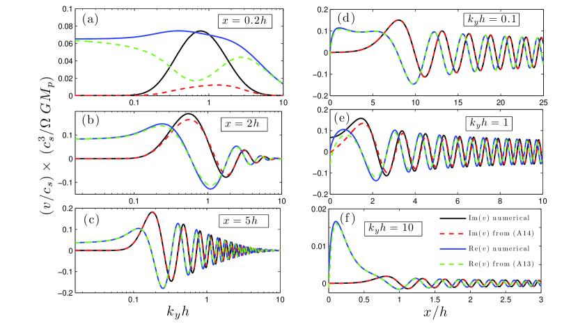
Figure 1.— Behavior of the individual Fourier harmonics of the azimuthal velocity perturbation $v$ as a function of both $k_{y}$ (left panels) and $x$ (right panels). Respective values of $x$ or $k_{y}h$ are shown in each panel. We plot $\Re(v)$ and $\Im(v)$ obtained both by the direct numerical integration of the equation (5) (solid curves) and using the Airy representation (dashed curves).

3.2. Analytical Airy representation.

In Appendix A we show that the solution of equation (10) with the boundary condition in the form of outgoing waves can be expressed in the limit $a\gg 1$ via the Airy functions, which have some algebraic function of $x$ as their argument, see equations (A2)-(A6). There we also derive the expressions (A13) and (A14) for the real and imaginary parts of $v$, which contain a number of exponentially small terms. Neglecting these terms, which is valid when $a\gg 1$, i.e. when either $k_{y}h\gg 1$ or $k_{y}h\ll 1$ one finds that the solution for $v$ reduces to

$$\Re(v)\sim-\frac{\pi g(z)}{a^{1/2}}\left[\mbox{Ai}(-t(z))\int\limits^{\infty}_{z}g(s)\mbox{Bi}(-t(s))R(s)ds+\mbox{Bi}(-t(z))\int\limits_{0}^{z}g(s)\mbox{Ai}(-t(s))R(s)ds\right],$$ (17)

$$\Im(v)\sim-\frac{\pi g(z)}{a^{1/2}}I_{+}\mbox{Ai}(-t(z)),$$ (18)

$$I_{+}=\int\limits_{0}^{\infty}g(s)\left[\mbox{Ai}(-t(s))-\frac{e^{-\pi a}}{2}\mbox{Bi}(-t(s))\right]R(s)ds.$$ (19)

Here Ai and Bi are Airy functions, while functions $g$ and $t$ are defined by equations (A5)-(A6).

We also demonstrate in Appendix A that whenever $k_{y}h\lesssim 1$ and $a\gtrsim 1$ the factor $I_{+}$ defined by equation (19) can be approximated for a Keplerian disk as

$$I_{+}=R(2\sqrt{a}h(3k_{y}h)^{-1/2})=-\frac{GM_{p}}{2\pi c}\left[wK_{0}\left(|w|\right)+\frac{1}{3}K_{1}\left(|w|\right)\right],~{}~{}~{}~{}~{}w=\frac{2}{3}\sqrt{1+(k_{y}h)^{2}}.$$ (20)

Equations (17)-(20) provide the foundation for our subsequent linear analytical study of the planet-generated density waves in §§4, 5.

3.3. Results.

In Figure 1 we show the behavior of the Fourier harmonics of the azimuthal velocity perturbation $v$ as a function of $x$ for a fixed $k_{y}$ and also as a function of $k_{y}$ for a fixed $x$. We display the behavior of $\Re(v)$ and $\Im(v)$ obtained by numerically solving equation (10), and also the analytical Airy representation of the same variable given by equations (A13)-(A14).

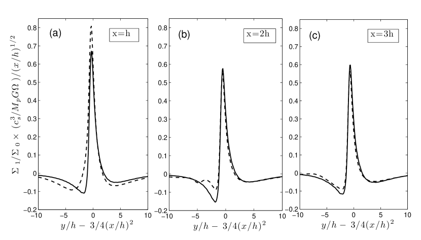
Figure 2.— Azimuthal cuts through the density wake in coordinate space showing the surface density perturbation $\Sigma_{1}$ at different radial separations from the planet ($x=h,2h,3h$ as labeled), normalized by $x^{1/2}$. Solid curves show numerical results while the dashed curves correspond to $\Sigma_{1}$ profiles obtained using Airy representation. An azimuthal shift by $(3/4)x^{2}$ is applied in each panel to facilitate comparison.

For a fixed $k_{y}$ satisfying the conditions $k_{y}h\lesssim 1$ or $k_{y}h\gtrsim 1$ (i.e. for $a\gtrsim 1$) the behavior of $v$ is reproduced by the Airy representation very well — in most cases the analytical prediction is hardly discernible from the numerical calculation, see Figures 1d,f. But as Figure 1e shows the Airy representation actually works quite well even for $k_{y}h\sim 1$ when formally it should not be applicable: analytical prediction falls essentially on top of the numerical results for both $\Re(v)$ and $\Im(v)$ as long as $x\gtrsim 5h$; significant discrepancy between the two is noticeable only for $x\lesssim 2h$.

Results for fixed $x$ tend to confirm this trend. Already at moderately large separations from the planet, e.g. $x=5h$, analytical predictions (A13)-(A14) reproduce the numerical results for all values of $k_{y}$ (including $k_{y}h\sim 1$) extremely well, see Figure 1c. Even at $x=2h$ the agreement is still pretty good, see Figure 1b, even though at this value of $x$ the modes with $k_{y}h\sim 1$ play the dominant role. It is only very close to the planet, e.g. at $x=0.2h$ as shown in Figure 1a, that the discrepancy between the Airy representation and the direct numerical calculation becomes significant, but again only for $k_{y}h\sim 1$ (analytical formulae agree with the numerical results in the limits $k_{y}h\ll 1$ and $k_{y}h\gg 1$ even at $x=0.2h$).

In Figure 2 we plot the behavior of the surface density perturbation $\Sigma_{1}(x,y)$ in physical space. We compute $\Sigma_{1}$ fully numerically by calculating its Fourier harmonics using equation (7) with numerically determined $v$ and then taking the inverse Fourier integral. We also calculate $\Sigma_{1}$ semi-analytically by repeating the same procedure with $\Re(v)$ and $\Im(v)$ given by equations (A13)-(A14). One can see that the two ways of computing $\Sigma_{1}(x,y)$ agree with each other quite well. They do show some discrepancy at small $x\approx h$, which is expected given the dominant role of the modes with $k_{y}h\sim 1$ in shaping the harmonic content of $\Sigma_{1}(x,y)$ close to the planet. However, further out from the planet the agreement between the Airy representation and the numerical calculation improves, see Figure 2c. Azimuthal density wave profiles at different separations from the planet have previously been computed by Goodman & Rafikov (2001) with the same method as we employ here, and by Dong et al. (2011) using direct numerical hydrodynamical simulations of tidal coupling between the low mass planet and the disk. Their results are in agreement with ours.

These comparisons clearly illustrate the robustness of the analytical Airy representation for the azimuthal velocity perturbation $v$ in certain limits. They also show that this representation can be used for accurate calculation of the behavior of the fluid variables in physical space at large $x/h$. All this gives us confidence in the subsequent use of this analytical approximation for the calculation of the asymptotic behavior of the torque density in §4 and the angular momentum flux in §5.

4. Torque density.

We now proceed to study the spatial behavior of the torque density $dT/dx$ — the amount of torque that is exerted by a planet on the disk per unit radial distance $x$. Analytical calculation of this important physical quantity has been first carried out by GT80 but only in the asymptotic regime $|x|\gtrsim h$. Besides, as we show below, this calculation was incorrect. Also, a number of numerical studies have derived $dT/dx$ for arbitrary $x$ as a by-product of their simulations (Bate et al. 2003; D’Angelo & Lubow 2008). Our current semi-analytical calculation is intended to provide the full description of $dT/dx$ in the linear regime for any $x$.

The torque density is defined as

$$\frac{dT}{dx}=-\int\limits_{-\infty}^{\infty}dy\Sigma_{1}\frac{\partial\Phi}{\partial y}.$$ (21)

Note that compared to $dT/dr$ this definition lacks an extra factor $r_{p}$ and strictly speaking represents the momentum density (even though we will still call it torque density in this work). This is because $r_{p}$ is not a well defined variable in the shearing sheet setup.

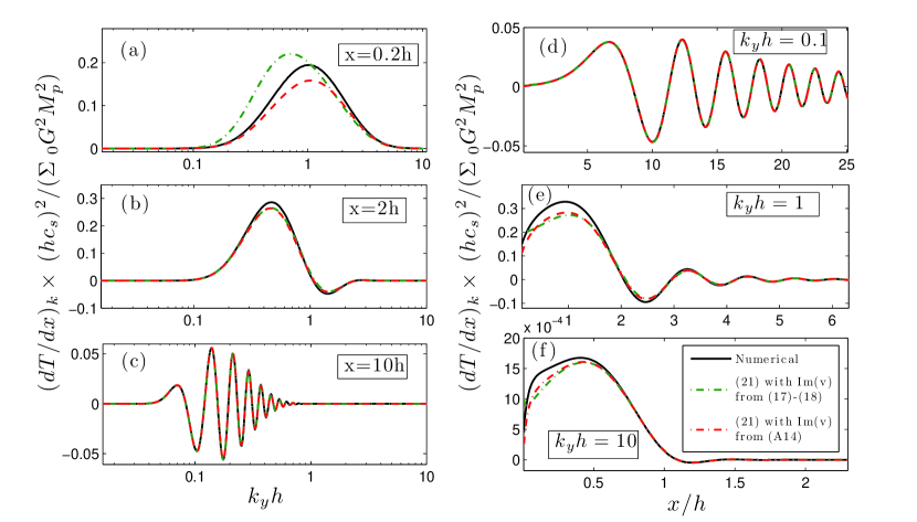
Figure 3.— Behavior of the individual Fourier harmonics of the torque density $(dT/dx)_{k}$ as a function of both $k_{y}$ (left panels) and $x$ (right panels), labeled correspondingly. Solid curves show numerical results while the dashed and dot-dashed curves represent $(dT/dx)_{k}$ obtained using different levels of the Airy representation (see text for details).

Fourier decomposing $\Sigma_{1}$ and $\Phi$ in azimuthal direction and manipulating the resultant expression we arrive at the following alternative expression:

$$\frac{dT}{dx}=\int\limits_{0}^{\infty}\left(\frac{dT}{dx}\right)_{k}dk_{y},$$

$$\left(\frac{dT}{dx}\right)_{k}=-4\pi k_{y}\phi\Im(\delta\Sigma)=-\frac{8\pi\Sigma_{0}}{k_{y}^{2}c^{2}+4B^{2}}k_{y}\phi\left[B\frac{\partial}{\partial x}\Im(v)-Ak_{y}^{2}x\Im(v)\right].$$ (22)

The last equality was derived using equation (7).

Our numerical solutions for the azimuthal velocity perturbation $v$ obtained in the previous section by numerically integrating the linear fluid equation (10) allow us to compute the individual Fourier harmonics $(dT/dx)_{k}$ using equation (22). In Figure 3 we show the behavior of $(dT/dx)_{k}$ as a function of both $k_{y}$ and $x$. We also display $(dT/dx)_{k}$ computed in the framework of the Airy representation using two levels of accuracy. Dot-dashed curve is derived from equation (22) using $v$ given by equation (18), which neglects the exponentially small terms, with $I_{+}$ given by equation (19). The $(dT/dx)_{k}$ shown by the dashed line uses $v$ given by equation (A14) in which all subdominant terms have been retained.

Again, we see very good agreement between the theoretical Airy representation and the numerical results in the limits of both $k_{y}h\gtrsim 1$ and $k_{y}h\lesssim 1$ for all $x$, as well as in the limit of $x\gtrsim h$ for any $k_{y}h$. This is in full agreement with the results for $v$ shown in Figure 1 since $(dT/dx)_{k}$ is directly derived from $v$ using (22). One can also see that the use of equation (A14) instead of (18) to represent $v$ gives a more accurate approximation of the numerical results. For that reason we generally recommend using the more accurate equation (A14) in semi-analytical calculations involving the Airy representation.

Next we explore the behavior of the full torque density $dT/dx$, integrated over all $k_{y}$ according to the equation (22). In Figure 4 we present the result of such calculation using numerically derived $v$. We also plot the analytical $dT/dx$ computed using Airy representation of $v$ at two levels of accuracy. First, simplified calculation (dot-dashed line) uses $\Im(v)$ given by equation (18) with $I_{+}$ computed according to the approximation (19). Not surprisingly this method of computing $dT/dx$ does not fare well at $x\sim h$ and it shows significant discrepancy with the numerical solution as $x/h\to 0$. Second, more accurate version of the Airy representation (dashed line) relies on equation (A14) retaining the exponentially small terms (which, however, become important as $k_{y}h\sim 1$) to describe the behavior of $\Im(v)$. This calculation yields better agreement with the numerical result as shown in Figure 4 even though there is still significant discrepancy (at the level of $10-20\%$) as $x\sim h$. At the same time, as expected based on the results of §3 both versions of the Airy representation work quite well at large separations from the planet, at $x\gtrsim 2h$.

We also plot in the Figure 4 $dT/dx$ derived from the direct numerical simulations of the disk-planet interaction (Dong et al. 2011). Clearly, the agreement between the linear theory results and the outcome of direct simulations is very good.

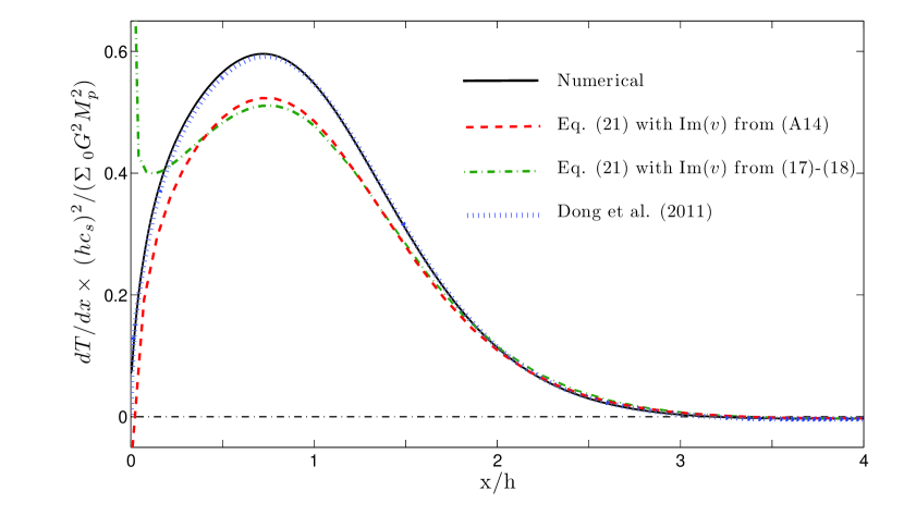
Figure 4.— Full torque density $dT/dx$ (integrated over all $k_{y}$) as a function of $x$ in the vicinity of the planet. Numerical linear results are given by solid line. Results obtained with the Airy representation (equation (22) integrated using $\Im(v)$ given by equation (A14)) are shown by dashed line, and those using $\Im(v)$ from equations (18)-(19) are shown by dot-dashed line. Dotted curve shows $dT/dx$ extracted from one of the numerical simulations of Dong et al. (2011).

4.1. Negative torque density phenomenon.

Different methods of calculating $dT/dx$ shown in Figure 4 universally exhibit the phenomenon of the negative torque density first described in Dong et al. (2011). Using direct numerical simulations these authors have shown that in a uniform disk $dT/dx$ changes sign at the finite separation from the planet in apparent disagreement with the predictions of GT80.

To illustrate this behavior in more detail in Figure 5a we show a zoomed-in view of $dT/dx$ at large separations $x>3h$. There we plot results of our numerical calculation, analytical calculation using Airy representation with $\Im(v)$ from equation (A14), and $dT/dx$ derived from the direct numerical simulations of Dong et al. (2001). All three methods of computing $dT/dx$ agree on the distance $x_{-}\approx 3.2h$ where $dT/dx$ changes sign. Linear theory results (both numerical and analytical) show good agreement with each other beyond this point while the $dT/dx$ derived from the direct hydrodynamical simulations exhibits some features related to numerical issues (mainly determined by the finite extent of the simulation domain in $x$-direction, see Dong et al. 2011).

We also show on this plot the asymptotic behavior of $dT/dx$ according to GT80 (thin solid line), see equation (2). It clearly disagrees with the linear results obtained in this work and with the results of the simulations by Dong et al. (2011) both in amplitude and the sign of the effect at $x\gtrsim 1$. We provide explanation for this discrepancy in §6.1.

In Appendix B we show using Airy representation of $v$ that the asymptotic behavior of the torque density in a Keplerian disk valid in the limit $x/h\to\infty$ is given by

$$\left(\frac{dT}{dx}\right)^{as} \to \mbox{sgn}(x)C\frac{(GM_{p})^{2}\Sigma_{0}}{\Omega^{2}}\frac{1}{x^{4}},$$

$$C = \frac{16}{81}\left[2K_{1}\left(\frac{2}{3}\right)-5K_{0}\left(\frac{2}{3}\right)\right]\left[2K_{0}\left(\frac{2}{3}\right)+K_{1}\left(\frac{2}{3}\right)\right]\approx-0.613096.$$ (23)

This expression replaces equation (2), which previously described the asymptotic behavior of $dT/dx$ according to GT80.

In Figure 5b we compare the asymptotic scaling given by equation (23) with the behavior of $dT/dx$ at large separations ($x<12h$) computed using our numerical determination of $v$ in equation (22). We also show on this plot $dT/dx$ obtained by numerically integrating the analytical expression (B4) over $k_{y}$. One can see that all three ways of representing the behavior of $dT/dx$ at large $x$ agree with each other quite well.

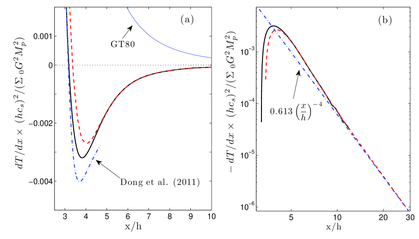
Figure 5.— Illustration of the negative torque density phenomenon. (a) Behavior of $dT/dx$ for $x>3h$ clearly showing change of sign of the torque density at $x_{-}\approx 3.2h$. Solid line stands for numerical linear calculation, dashed curve is for Airy representation with $\Im(v)$ given by equation (A14), and dot-dashed line shows the results of simulations (Dong et al. 2011). Thin solid line shows the asymptotic prediction of GT80. (b) Asymptotic behavior of $dT/dx$ at large $x/h$ (note the negative sign). Solid curve is the same as in panel (a), dot-dashed line shows asymptotic behavior (23), and dashed line results from integrating equation (B4) over $k_{y}$.

5. Angular momentum flux.

To get the full picture of the disk evolution driven by planet-generated density waves it is important to properly understand not only the wave damping mechanisms but also the amount of the angular momentum carried by the waves — angular momentum flux $F_{H}$, and its spatial pattern.

Total angular momentum flux carried by the density wave is

$$F_{H}=\Sigma_{0}\int\limits_{-\infty}^{\infty}dy~{}v_{x,1}v_{y,1}=\int\limits_{0}^{\infty}F_{H,k}dk_{y},~{}~{}~{}~{}~{}F_{H,k}=4\pi\Sigma_{0}\left[\Re(v)\Re(u)+\Im(v)\Im(u)\right]=4\pi\Sigma_{0}\Re\left(uv^{*}\right),$$ (24)

where $F_{H,k}$ is the angular momentum flux carried by a particular azimuthal mode of the wave, and $*$ denotes complex conjugate. Using equation (6) and the fact that $\phi$ is purely real we find

$$F_{H,k}=-\frac{4\pi\Sigma_{0}}{k_{y}^{2}c^{2}+4B^{2}}\left[k_{y}c^{2}\Re\left(iv^{*}\frac{\partial v}{\partial x}\right)+2Bk_{y}\phi\Im(v)\right]$$ (25)

Because of the angular momentum conservation the radial divergence of the angular momentum flux $dF_{H,k}/dx$ must be equal to $(dT/dx)_{k}$. To demonstrate this property we differentiate equation (25) with respect to $x$ and then transform the term proportional to $v^{*}\partial v/\partial x$ using equation (5). In the end we find that $dF_{H,k}/dx$ is indeed given by the same expression in terms of $\Im(v)$ as $(dT/dx)_{k}$, see equation (22).

In the important limit $x\to\infty$ we can compute the asymptotic value of the angular momentum flux harmonic $F_{H,k}$ analytically. For this purpose we use equation (25), in which $\phi\to 0$ as $x\to\infty$ (see equation (11)), so that

$$F_{H,k}(x\to\infty)\to\frac{4\pi\Sigma_{0}k_{y}c^{2}}{k_{y}^{2}c^{2}+4B^{2}}\left[\Re(v)\frac{\partial}{\partial x}\Im(v)-\Im(v)\frac{\partial}{\partial x}\Re(v)\right].$$ (26)

In the same limit $x,z\to\infty$ equation (17) reduces to

$$\Re(v)\sim-\frac{\pi g(z)}{a^{1/2}}I_{+}\mbox{Bi}(-t(z)),$$ (27)

where $I_{+}$ is given by equation (19). The exponentially small contributions present in equation (A13) have been dropped from this expression.

Using these facts we show in Appendix C that the Fourier component of the angular momentum flux is given in the limit $k_{y}h\lesssim 1$ and $x/h\gg 1$ by the following formula in a Keplerian disk:

$$F_{H,k}(x\to\infty)=\frac{4}{3}k_{y}^{2}\frac{(GM_{p})^{2}\Sigma_{0}}{\Omega^{2}}\left[2K_{0}\left(\frac{2}{3}\right)+K_{1}\left(\frac{2}{3}\right)\right]^{2}.$$ (28)

This expression coincides with the corresponding result of GT80 obtained in the limit $m\lesssim r/h$ (see their equation (91)).

In Figure 6 we present the run of the full angular momentum flux $F_{H}(x)$ in real space, as a function of the radial separation from the planet. One can see that $F_{H}$ starts with a non-zero value of $0.098$ (in units of $(G^{2}M_{p}^{2}\Sigma_{0})/(hc^{2})$) at $x=0$ and then gradually rises until $x$ is about $3$. Beyond that point $F_{H}(x)$ starts decreasing with the distance although the decline is rather modest: the peak value of $F_{H}$ is $0.938$ (in the same natural units) while the value of $F_{H}$ at $x=15h$ is about $0.908$. This reduction of $F_{H}(x)$ with the distance is a direct consequence of the negative torque density phenomenon discussed in §4.1, since $dF_{H}/dx=dT/dx$ as we have shown before. The latter point is additionally emphasized in Figure 6 where we also plot the integrated torque $T(x)\equiv\int_{0}^{x}(dT/dx)dx$. One can see that $F_{H}(x)$ and $T(x)$ are identical to each other up to the vertical shift by $F_{H}(0)$.

Previously, using calculation in the Fourier space, GT80 have found $F_{H}(\infty)=0.93$, which is close to the value we find. The small difference between these numbers might possibly be ascribed to the small $k_{y}$ range used by GT80 to compute $F_{H}(\infty)$ and should not be taken too seriously.

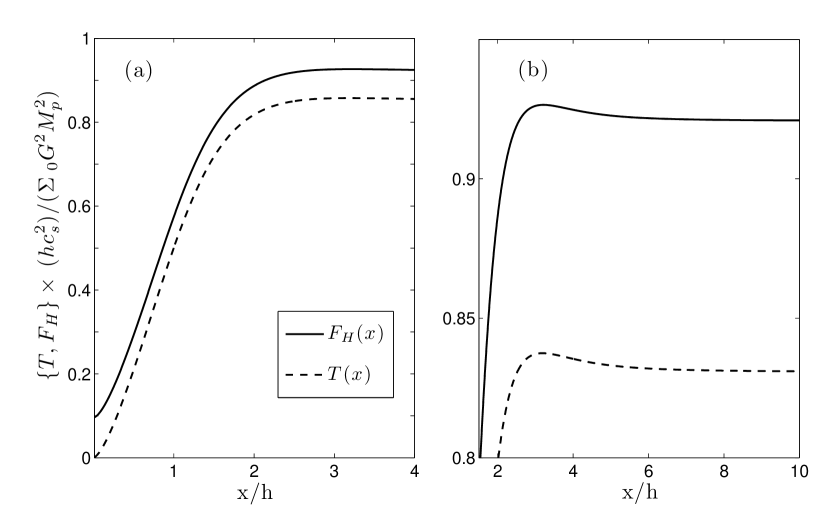
Figure 6.— (a) Scaling of the angular momentum flux $F_{H}$ with the distance from the planet (solid curve). We also plot integrated torque $T(x)$ accumulated by the wave at distance $x$ (dashed curve). Note that $F_{H}(x)$ has a non-zero value at $x=0$, and that $dT/dx=dF_{H}/dx$. (b) Close-up view at $x>2h$ to illustrate the slight decay of $F_{H}(x)$ and $T(x)$ at large $x$ as a result of the negative torque density phenomenon (see §4.1).

6. Discussion.

Most of the existing linear calculations of the disk-satellite coupling have been limited to the Fourier space (Ward 1986; Artymowicz 1993; Tanaka et al. 2002). Notable exceptions include Meyer-Vernet & Sicardy (1987) who discussed the radial structure of the perturbed velocity eigenfunctions for a fixed azimuthal wavenumber under a variety of assumptions about the physics operating in the disk. Later on KP93 have done similar calculation for a disk with non-zero pressure (the same setup as used in our current work) and computed the run of $F_{H,k}$ as a function of $x$. But these studies have only looked at the spatial behavior of individual modes driven by the planetary potential.

More recently Goodman & Rafikov (2001) have integrated the contributions of separate modes over the azimuthal wavenumber to obtain the full spatial distribution of the perturbed surface density. Our current work extends the study Goodman & Rafikov (2001) by computing the spatial behavior of other important fluid variables such as the torque density and the angular momentum flux.

The key result of our present study is the confirmation of the negative torque density phenomenon (discovered in the numerical study of Dong et al. (2011)) in the framework of the linear theory of disk-satellite interaction, and the determination of the asymptotic behavior of $dT/dx$ far from the planet. The discrepancy between our result (23) and the conventional expression (2) not just in amplitude of the effect but also in its sign quite naturally demands an explanation, which we provide below.

6.1. Origin of the negative torque density.

All calculations of the torque and angular momentum flux excited by the planet in GT80 have been carried out in Fourier space for individual harmonics of the planetary potential. These results fully agree with our calculations in §§4 & 5, in particular we successfully reproduce their expression for $F_{H,k}$ in §5. However, GT80 also tried to convert their results on torque exerted by the planet to physical (coordinate) space, and in doing this they had to resort to certain assumptions. In particular, they postulated that the action of each potential harmonic, including the deposition of a corresponding torque contribution, is localized in the vicinity of a respective Lindblad resonance. Under this assumption they computed the torque density at each location in physical space as the simple product of the spatial density of Lindblad resonances $|dk_{y}/dx|$ and the amplitude of the torque component in Fourier space $T_{k}\equiv\int_{-\infty}^{\infty}(dT/dx)_{k}dx$, corresponding to $k_{y}$ with Lindblad resonance at this particular location (i.e. at $k_{y}=2/(3x)$). Equation (2) represents the result of such a calculation in the limit $x/h\gg 1$. Not surprisingly, one finds the sign of $(dT/dx)^{\rm LR}$ to be the same for any $x$ simply because the Fourier amplitudes of the torque have the same sign independent of $m$ — there is no disagreement on this issue between us and GT80.

What we find in this work is that the Fourier contribution to the torque density of each azimuthal harmonic of the potential $(dT/dx)_{k}$ is in fact spread out over a finite portion of the disk, rather than localized in a narrow region around each Lindblad resonance. In this situation, the overlap of many Fourier modes at a given point in space is inevitable and the calculation of the full torque density in real space represents a rather challenging task, requiring direct integration of the equation (22). As a result of carrying out this exercise, one finds the distribution of the torque density different from (2) at large values of $x$, as clearly demonstrated in Figure 5a.

This reasoning is best illustrated if we temporarily abandon the shearing sheet approximation and consider the disk-satellite interaction in the full cylindrical geometry. Then, as pointed out by GT80, coupling between the planetary potential and the disk occurs at discrete Lindblad resonances radially separated from the planetary orbit by $x_{L,m}\approx 2r_{p}/(3m)$, where $m=k_{y}r_{p}$ in the azimuthal wavenumber of the potential harmonic and an assumption $m\gtrsim 1$ has been made. The distance between the adjacent $m$-th and $(m+1)$-th resonances is $\Delta x_{L,m}=x_{L,m}/m=x_{L,m}(h/r_{p})(k_{y}h)^{-1}$.

We need to compare this distance to the width $\delta x_{m}$ of the $m$-th resonance. According to Airy representation (see §3.2 and Appendix A) the latter is set by the condition $t\sim 1$ or $2a^{2/3}(\xi-1)\sim 1$ (valid near the Lindblad resonance), see equations (A5) and (A15). One then finds that the resonance width $\delta x_{m}$ is given by $\delta x_{m}\sim x_{L,m}a^{-2/3}\sim x_{L,m}(k_{y}h)^{2/3}$ for $k_{y}h\lesssim 1$. Note that $\delta x_{m}\ll x_{L,m}$.

A somewhat more illuminating way of deriving $\delta x_{m}$ is based on the dispersion relation for the tightly wound density waves (Binney & Tremaine 2008), which is valid for $m\gtrsim 1$ or $k_{y}h\gtrsim(h/r)$:

$$\kappa^{2}+k_{r}^{2}c_{s}^{2}=m^{2}(\Omega-\Omega_{p})^{2}\approx\frac{4m^{2}A^{2}}{r_{p}^{2}}x^{2},$$ (29)

where $k_{r}$ is the radial wavenumber of the wave. The exact resonance location $x_{L,m}=r_{p}m^{-1}(\kappa/2|A|)$ corresponds to the distance where $k_{r}=0$ and the wave couples best to the external potential. As the radial separation from the resonance increases $k_{r}$ grows until at $|x-x_{L,m}|\sim\delta x_{m}$ one gets $k_{r}\delta x_{m}\sim 1$. Beyond this point the wave eigenfunction starts oscillating rapidly, and coupling to the external potential becomes less effective. Plugging $k_{r}\sim\delta x_{m}^{-1}$ and $x=x_{L,m}+\delta x_{m}$ into the dispersion relation (29) and expanding it in terms of $\delta x_{m}\ll x_{L,m}$ one finds $\delta x_{m}\sim h(k_{y}h)^{-1/3}$, the same expression as that as resulting from the Airy representation.

Using these estimates of $\Delta x_{L,m}$ and $\delta x_{m}$ one can easily see that $\delta x_{m}\gtrsim\Delta x_{L,m}$ and resonances located at distance $x$ from the perturber overlap as long as

$$x\lesssim h\left(\frac{r_{p}}{h}\right)^{3/5}=r_{p}\left(\frac{h}{r_{p}}\right)^{2/5}.$$ (30)

Equivalently, overlap occurs for modes having

$$k_{y}h\gtrsim\left(\frac{h}{r_{p}}\right)^{3/5}~{}~{}~{}~{}\mbox{or}~{}~{}~{}~{}m\gtrsim\left(\frac{r_{p}}{h}\right)^{2/5}.$$ (31)

Interference of different modes takes place even though the width of each resonance $\delta x_{m}$ is small compared to the resonance separation $x_{L,m}$ from the perturber’s orbit.

Thus, whenever $r_{p}/h\gg 1$, which is always the case for protoplanetary and many other kinds of accretion disks, resonances overlap in the vicinity of the perturber’s orbit (for $x$ satisfying equation (30)) and the assumption of well-isolated resonances adopted by GT80 for their torque density calculation fails. Given that in our calculation the negative values of $dT/dx$ appear only for $x>x_{-}\approx 3.2h$ (see §4.1) one needs the inverse of the disk aspect ratio to be $r_{p}/h\gtrsim(x_{-}/h)^{5/3}\approx 7$ for the negative $dT/dx$ to appear. This requirement is easily fulfilled in a large variety of astrophysical accretion disks, including protoplanetary disks.

In the framework of the shearing sheet approximation, which corresponds to the limit $r_{p}/h\to\infty$, it is not surprising, according to equation (30), that resonances overlap for all $x$ and the isolated resonance approximation adopted in GT80 never holds. In this limit our asymptotic expression (23) works fine for arbitrary $x$.

At the same time, far from the perturber’s orbit, at separations not obeying the condition (30) resonances become sufficiently spread apart to act in isolation. In this case one would expect the GT80’s expression (2) to be valid. Thus, when the full cylindrical geometry of the disk-planet interaction is accounted for $dT/dx$ at fist becomes negative close to the planet, for $x>x_{-}$, but then should change sign and become positive again (outside of the region defined by the inequality (30)) in accordance with the GT80 calculation. The details of this transition can only be elucidated via linear calculation of the disk-planet coupling in the cylindrical geometry, which is beyond the scope of this work.

6.2. Comparison with previous work.

Quite interestingly, the existence of the negative torque density phenomenon could have been inferred from calculations done even prior to the work of Dong et al. (2011). In particular, Bate et al. (2003) performed global three-dimensional simulations of the disk-planet interaction in cylindrical geometry. As a part of this calculation they have computed torque density produced by planets of different masses. Close inspection of their Figure 12 shows that at small masses, $M_{p}\lesssim 0.03$ M_J, the torque density changes sign at a finite separation from the planet. This effect does not disappear as $M_{p}$ is reduced strongly suggesting that it is a linear phenomenon.

More recently D’Angelo & Lubow (2008) have computed radial run of $dT/dx$ as one of the by-products of their three-dimensional global simulations. In their Figure 7 one can again see the torque density changing sign for low enough $M_{p}\lesssim 10$ M_⊕, which is in good agreement with the torque density behavior that could have been inferred from the work of Bate et al. (2003). Similar torque density pattern can also be seen in D’Angelo & Lubow (2010).

Finally, Muto & Inutsuka (2009) have carried out a local linear analysis of interaction between a planet and the surrounding viscous disk. Even though their results are affected to some extent by the assumed non-zero value of viscosity (our study assumes viscosity to be zero), their torque density still exhibits negative values beyond $x\approx 3h$ (see their Figure 5) even at the lowest values of viscosity, in agreement with our work.

The most likely reason for why the negative torque density phenomenon went unnoticed in previous studies lies in the small amplitude of this effect. Indeed, the total negative torque contribution obtained by integrating $dT/dx$ from $x_{-}\approx 3.2h$ to $\infty$ amounts to $\lesssim 4\%$ of the total integrated torque $T(\infty)=\int_{0}^{\infty}(dT/dx)dx$. Thus, it is not surprising that this real effect was previously ignored, most likely on the basis of it being due to some numerical issues (poor resolution, small simulation box size, etc.).

Nevertheless, the apparent presence of the negative torque phenomenon in the aforementioned earlier works provides additional support for the robustness of the results presented in this paper. In particular, one may wonder whether our conclusions based on a linear calculation performed in two-dimensional shearing sheet geometry would hold when some of our assumptions — local approximation, linearity of the perturbation, two-dimensional geometry — are relaxed. In this regard we simply point out here that both Bate et al. (2003) and D’Angelo & Lubow (2008) ran three-dimensional, global simulations for a variety of planetary masses and one can still discern the presence of the negative torque phenomenon in their results. This gives us reassurance in the ubiquity of this rather subtle but important (see §7) feature of the disk-planet interaction even in more sophisticated and realistic geometries.

6.3. Accuracy of the Airy representation.

Another interesting result of our study concerns the accuracy with which the analytical Airy approximation described in §3.2 and Appendix A characterizes the details of the disk-planet interaction. Approximation of the behavior of the perturbed fluid variables in terms of Airy functions has been used by many authors before (Artymowicz 1993; Ward 1986) but only to represent the behavior in the vicinity of Lindblad resonances. As such the Airy representation served only as a local analytical tool for computing the azimuthal Fourier components of the density wave properties such as the angular momentum flux.

In our study we use Airy representation in a global sense, to describe the spatial variation of the fluid variables for the values of $x$ not limited to the locations of the Lindblad resonances. This procedure works well for describing the behavior of the Fourier harmonics of the azimuthal velocity perturbation $v$ and of the torque density $dT/dx$ at any $x$ as long as the wavenumber of a particular mode satisfies the condition $a\gtrsim 1$, which according to equation (12) is true whenever $k_{y}h\lesssim 1$ or $k_{y}h\gtrsim 1$. Moreover, for $x\gtrsim h$ this approximation is quite reliable even for $k_{y}h\sim 1$. As a result the Airy representation successfully reproduces the asymptotic behavior of $dT/dx$ and $F_{H,k}$ as a function of $x$ in the limit $x/h\gg 1$ as we have shown in §4.1 and §5. And as Figures 2 and 4 demonstrate one can also use Airy representation to reproduce with decent accuracy the density wave properties in physical space.

These conclusions are in agreement with the results of Heinemann & Papaloizou (2011) who found that the WKBJ approximation valid whenever $a\gtrsim 1$ works very well for describing the evolution of the spiral density waves excited by the turbulence in the disk.

7. Astrophysical implications.

Understanding the negative torque density phenomenon (see §4.1) in uniform disks is the major result of our work. It is natural to ask whether this effect can somehow change global consequences of the disk-satellite interaction in real disks.

It is known that planets, which are not massive enough to open a gap around their orbit can migrate radially because of the small asymmetry of their gravitational coupling to the inner and outer parts of the disk (GT80); this is the so-called Type I migration (Ward 1997). In our shearing-sheet setup such asymmetry is absent by construction and planets do not migrate. But the negative torque density is still going to be present in real disks (which are close to being uniform locally, near the planet) and one may wonder whether it may affect the speed of Type I migration. The answer is no, because the speed of migration is insensitive to the spatial structure of $dT/dx$ and depends only on the difference of the full one-sided torques exerted on the inner and outer portions of the disk. As we have shown in §5 the one-sided torque is not changed in our calculation compared to the GT80 prediction, so the speed of Type I migration stays the same as long as the disk is roughly uniform.

Deposition of the angular momentum carried by the density waves drives evolution of the disk away from its initially uniform state. This evolution depends on the spatial pattern of $dT/dr|_{d}$ (see equation (1)) representing the wave angular momentum that is being deposited in the disk material. According to equation (1) the latter quantity depends not only on $dT/dx$ which describes the driving of the waves but also on the process that leads to their damping and transfer of the wave angular momentum to the disk material (Takeuchi et al. 1996; Rafikov 2002). However, once the latter is understood (i.e. the explicit form of operator ${\cal L}$ in equation (1) is determined) the disk evolution is going to be fully determined by the dependence of $dT/dx$ on $x$, and thus should be directly affected by the negative torque density phenomenon.

The influence of this effect on $dT/dr|_{d}$ should depend on the details of the damping process. Since the negative torque density is a rather small effect (the full amount of negative torque is just several per cent of the full torque, see §5) it should not affect $dT/dr|_{d}$ if the damping is weak and the characteristic distance over which wave is dissipated is $l_{d}\gg h$. What happens in the case of strong damping, when $l_{d}$ becomes comparable to the distance between individual Lindblad resonances, is not so obvious. In particular, it is not clear whether $dT/dr|_{d}$ should become negative at $|x|\gtrsim x_{-}$ as does $dT/dr$, or whether $dT/dr|_{d}$ will tend to converge to the GT80 prediction (2). This issue can be addressed in the future by calculations making explicit assumptions about the damping mechanism. And one should keep in mind that strong damping can affect not only propagation of the waves but also their excitation in a non-trivial way (Muto & Inutsuka 2009).

It is worth mentioning that, with the rare exceptions of the works by Takeuchi et al. (1996) and Rafikov (2002), in the majority of studies of the perturber-driven disk evolution the wave damping process is essentially ignored and it is assumed that the amount of angular momentum transferred to the disk material is given simply by $dT/dr$ (e.g. Lin & Papaloizou 1986; Chang et al. 2010), i.e. the assumption $dT/dr|_{d}=dT/dr$ is usually made. However, the circumstances under which such assumption is justified have never been explicitly clarified. In general the correct approach to understanding the disk evolution due to tidal interaction must incorporate both the correct form of $dT/dr$ (or $dT/dx$) and the description of the wave damping. If the latter is ignored then according to Goldreich & Nicholson (1989) the disk should not evolve at all.

Knowledge of the spatial behavior of the torque density $dT/dx$ (or $dT/dr$) produced by a perturber is one of the key ingredients for understanding the process of gap opening. In particular, in steady state the shape of the gap is uniquely determined by the balance of the viscous torque density in the disk and the radial divergence of the angular momentum flux carried by the density waves $dT/dr|_{d}$.

A proper calculation of the gap shape is important not only in itself but also for computing the full torque exerted by the perturber on the disk. If this torque is non-zero (e.g. due to the disk being absent on one side) then the perturber will migrate (Type II migration in presence of a gap, see Ward (1997)) as a result of the angular momentum conservation. The speed of migration depends on the shape of the gap since the surface density profile is one of the ingredients determining how much net torque the perturber deposits in the disk (Ward 1997).

Calculation of the excitation torque density $dT/dx$ in a non-uniform disk must be modified compared to that in the constant $\Sigma$ disk. This is usually accomplished by computing $dT/dx|_{\rm nu}$ in a non-uniform disk according to the following prescription:

$$\frac{dT(x)}{dx}\Bigg{|}_{\rm nu}=\Sigma(x)\frac{1}{\Sigma_{0}}\frac{dT(x)}{dx}\Bigg{|}_{\rm u},$$ (32)

where $dT/dx|_{\rm u}$ is the torque density in a uniform disk, a quantity which is the subject of the calculations done in GT80 and in our work (where we call it just $dT/dx$). One normally uses the GT80’s prescription (2) for $dT/dx|_{\rm u}$ (Lin & Papaloizou 1986; Trilling et al. 1998; Armitage & Natarajan 2002; Armitage et al. 2002; Lodato et al. 2009) or a modified version thereof. Given that in this case the torque density has a definite sign, the tidal interaction between the perturber and the gap edges is repulsive and the planet drives a positive angular momentum flux through the disk, which is consistent with the gap opening picture.

Our revision of the $dT/dx$ calculation and the discovery of the negative torque density phenomenon might be thought of as giving rise to an interesting paradox. With our new expression (23) for the torque density one may think that equation (32) predicts $dT/dx|_{\rm nu}<0$ for $x>x_{-}\approx 3.2h$. Then the application of the prescription (32) for computing the full torque in a broad gap with width exceeding $2x_{-}$ would result in the negative angular momentum flux accumulated by the wave and the attractive interaction between the planet and the fluid at the gap edges. Apparently, under such circumstances the gap would not be able to appear in the first place.

The resolution of this apparent paradox lies in the use of the prescription (32) to describe the torque density in an inhomogeneous disk. Indeed, the calculation of $dT/dx|_{\rm u}$ is based on the solutions of the perturbed fluid equations (5)-(7) derived under the assumption of a uniform density. However, in a non-uniform disk these equations get modified and new terms caused by the gradients of $\Sigma$ appear in them. These terms are especially important at the steep edges of gaps or cavities. Their presence significantly modifies the structure of the velocity eigenfunctions and makes the prescription (32) irrelevant. In general one should not expect equation (32) to provide correct results even for the excitation torque density $dT/dx$ (not mentioning the torque density $dT/dx|_{d}$ deposited in the disk by the density wave).

A fully self-consistent calculation of $dT/dx|_{\rm nu}$ should be based on equations explicitly incorporating disk non-uniformity and thus has little to do with $dT/dx|_{\rm u}$. An example of such a self-consistent linear calculation of $dT/dx|_{\rm nu}$ is provided in Petrovich & Rafikov (2012; in preparation) where it is shown that a proper account of the disk non-uniformity in fluid equations results in the positive angular momentum flux produced by the perturber and the repulsion of fluid away from its orbit for gaps of arbitrary width.

Knowledge of the behavior of the torque density $dT/dr$ is also important for determining the surface density profile in cavities or gaps formed in accretion disks by embedded binary SMBHs. In the case of extreme mass ratio inspirals the gap formed by the lower mass BH can be quite narrow (Chang et al. 2010) so that the results obtained in the local shearing sheet approximation remain valid. In particular, the negative torque density phenomenon may be relevant for this type of objects if the mass of the secondary is insufficient to significantly perturb the disk surface density and open a gap.

However, in the case of SMBHs of comparable mass the binary usually clears out a large cavity with inner radius comparable to the binary separation in the disk around itself (MacFadyen & Milosavljević 2008; Shi et al. 2011). In that case understanding the torque density distribution requires one to carry out a global calculation of the density wave excitation by the binary in a highly non-uniform disk in full cylindrical geometry. But even in this much more complicated setting one may still use the intuition gained in our present study. In particular, equation (30) suggests that the negative torque phenomenon is not going to be important since the range of $x$ where the resonances overlap falls inside the cavity. At the inner edge of the cavity, at separations of order the binary semi-major axis the resonances are well isolated and procedure adopted in GT80 to compute $dT/dr$ may actually work.

On the other hand, if the cavity is very wide then the torque is generated by only a handful of individual modes since only a small number of low-$m$ Lindblad resonances are going to be located in the region with appreciable gas surface density. As a result, the pattern of $dT/dx$ may be more reminiscent of the $(dT/dx)_{k}$ corresponding to a single azimuthal Fourier harmonic of the potential, which usually exhibits complicated oscillatory pattern, see upper right panel in Figure 3 and KP93. This expectation agrees well with the results of numerical simulations of MacFadyen & Milosavljević (2008), Cuadra et al. (2009), Farris et al. (2011), and Shi et al. (2011) who have found oscillating $dT/dx$ in disks with large cavities cleared by the SMBH binaries.

8. Summary.

We have carried out linear calculation of the gravitational coupling between the uniform gaseous disk and an embedded massive perturber. Our work goes beyond similar earlier studies by putting emphasis on understanding the behavior of the perturbed fluid variables in real space as opposed to Fourier space. This allows us to address the nature of the recently discovered negative torque phenomenon and explain its origin fully in the framework of linear theory.

We come up with the global analytical representation of the spatial variation of the perturbed fluid variables in terms of the Airy functions, which is shown to work quite well for describing the properties of the planet-generated density waves both in Fourier and in real space. Using this approximation we derive the asymptotic behavior of the torque density far from the perturber and show that it matches the results of numerical calculations. Our linear calculations confirm that the torque density changes sign at a finite separation from the perturber in full agreement with the results of the direct hydrodynamical simulations. This provides an important correction to the calculations of GT80.

These results have broad implications for understanding tidal interaction of planets with circumstellar disks and of binary SMBHs with the circumbinary accretion disks. In particular, our calculations provide a pathway for deriving the spatial torque distributions in such disks, which is important for understanding the issues of gap opening by planets and gas clearing by binary SMBHs.

Appendix A Airy representation.

The following results extensively use the relations presented in Chapter 19 of Abramowitz & Stegun (1972; hereafter AS). Homogeneous parabolic cylinder equation

$$\frac{\partial^{2}v}{\partial X^{2}}+v\left(\frac{X^{2}}{4}-a\right)=0,$$ (A1)

i.e. the equation (10) with $R$ set to zero has two independent homogeneous solutions, which behave as purely outgoing waves at infinity (Narayan et al. 1987):

$$v_{+}=E(a,X)=\mbox{k}^{-1/2}W(a,X)+i\mbox{k}^{1/2}W(a,-X),$$

$$v_{-}=E^{\star}(a,-X)=\mbox{k}^{-1/2}W(a,-X)-i\mbox{k}^{1/2}W(a,X),$$ (A2)

$$\mbox{k}\equiv\sqrt{1+e^{2\pi a}}-e^{\pi a},$$ (A3)

where $W(a,X)$ is the standard solution of equation (A1), see chapter 19.17 of AS. One can easily show that the Wronskian $\Delta=W\left\{E(a,X),E^{\star}(a,-X)\right\}=2e^{\pi a}$ is independent of $X$.

In chapter 19.20 of AS it is shown that when $a$ is large and positive ($a\gg 1$) the parabolic cylinder function $W(a,X)$ can be expressed via Airy functions for any $X>0$ in the following way:

$$W(a,X)\sim\sqrt{\pi}\frac{e^{-\pi a/2}}{(4a)^{1/4}}g(X)\mbox{Bi}(-t),~{}~{}~{}~{}~{}~{}W(a,-X)\sim 2\sqrt{\pi}\frac{e^{\pi a/2}}{(4a)^{1/4}}g(X)\mbox{Ai}(-t),$$ (A4)

where

$$\xi(X) \equiv \frac{X}{2\sqrt{a}},~{}~{}~{}~{}~{}t(\xi)\equiv(4a)^{2/3}\tau(\xi),~{}~{}~{}~{}~{}g(X)\equiv\left[\frac{t(\xi)}{\xi^{2}-1}\right]^{1/4}$$ (A5)

$$\tau(\xi) = -\left(\frac{3}{8}\right)^{2/3}\left(\mbox{arccos}~{}\xi-\xi\sqrt{1-\xi^{2}}\right)^{2/3},~{}~{}~{}~{}~{}~{}\xi\leq 1,$$ (A6)

$$= \left(\frac{3}{8}\right)^{2/3}\left(\xi\sqrt{\xi^{2}-1}-\mbox{arccosh}~{}\xi\right)^{2/3},~{}~{}~{}~{}~{}~{}\xi\geq 1.$$

We will also need to know the asymptotic behavior of Airy functions as $X\to\infty$ (here $\zeta\equiv(2/3)X^{3/2}$):

$$\mbox{Ai}(X)\sim\frac{e^{-\zeta}}{2\sqrt{\pi}X^{1/4}},~{}~{}~{}~{}~{}\mbox{Bi}(X)\sim\frac{e^{\zeta}}{\sqrt{\pi}X^{1/4}},$$

$$\mbox{Ai}(-X)\sim\frac{\cos(\zeta-\pi/4)}{\sqrt{\pi}X^{1/4}},~{}~{}~{}~{}~{}\mbox{Bi}(-X)\sim-\frac{\sin(\zeta-\pi/4)}{\sqrt{\pi}X^{1/4}}.$$ (A7)

Full solution of inhomogeneous equation (10) behaving as purely outgoing wave for $x\to\pm\infty$ is expressed via the homogeneous solutions $v_{\pm}$ as

$$v(k_{y},x)=-\frac{v_{+}}{\Delta}\int\limits_{-\infty}^{z}v_{-}(s)R(s)ds-\frac{v_{-}}{\Delta}\int\limits^{\infty}_{z}v_{+}(s)R(s)ds.$$ (A8)

Here it is understood that $z=z(x)$ and $R(s)=R(x(s))$, where the corresponding dependencies are given by equations (9) and (11).

Now we consider the behavior of the solutions for positive $x$ (and $z$). For $a\gtrsim 1$ and $z>0$ one can write using equations (A2)-(A4)

$$v_{+} \sim \sqrt{2}e^{\pi a/2}W(a,z)+i\frac{e^{-\pi a/2}}{\sqrt{2}}W(a,-z)\sim\frac{\sqrt{\pi}}{a^{1/4}}g(z)\left[\mbox{Bi}(-t(z))+i\mbox{Ai}(-t(z))\right],$$ (A9)

$$v_{-} \sim \sqrt{2}e^{\pi a/2}W(a,-z)-i\frac{e^{-\pi a/2}}{\sqrt{2}}W(a,z)$$ (A10)

$$\sim \frac{\sqrt{\pi}}{a^{1/4}}g(z)\left[2e^{\pi a}\mbox{Ai}(-t(z))-i\frac{e^{-\pi a}}{2}\mbox{Bi}(-t(z))\right],$$

where $\xi=z/(2\sqrt{a})$ and $t(z)$ implies $t$ calculated with this value of $\xi$.

Integrals in equation (A8) involve integration over both positive and negative $z$ (or $x$), so we need the Airy function approximation for $v_{\pm}$ for negative arguments as well:

$$v_{+} \sim \sqrt{2}e^{\pi a/2}W(a,-|z|)+i\frac{e^{-\pi a/2}}{\sqrt{2}}W(a,|z|)$$ (A11)

$$\sim \frac{\sqrt{\pi}}{a^{1/4}}g(-z)\left[2e^{\pi a}\mbox{Ai}(-t(-z))+i\frac{e^{-\pi a}}{2}\mbox{Bi}(-t(-z))\right],$$

$$v_{-} \sim \sqrt{2}e^{\pi a/2}W(a,|z|)-i\frac{e^{-\pi a/2}}{\sqrt{2}}W(a,-|z|)$$ (A12)

$$\sim \frac{\sqrt{\pi}}{a^{1/4}}g(-z)\left[\mbox{Bi}(-t(-z))-i\mbox{Ai}(-t(-z))\right],$$

where now $z<0$, $\xi=-z/(2\sqrt{a})$, and $t(-z)$ means $t$ computed with this value of $\xi$.

Plugging the expressions (A11)-(A10) into equation (A8) we find that for $a\gg 1$ and $z>0$

$$\Re(v) \sim -\frac{\pi g(z)}{a^{1/2}}\left\{\mbox{Ai}(-t(z))\left[\int\limits^{\infty}_{z}g(s)\mbox{Bi}(-t(s))R(s)ds+\frac{e^{-2\pi a}}{4}\int\limits^{z}_{0}g(s)\mbox{Bi}(-t(s))R(s)ds\right.\right.$$ (A13)

$$- \left.\left.\frac{e^{-\pi a}}{2}\int\limits^{\infty}_{0}g(s)\mbox{Ai}(-t(s))R(s)ds\right]+\mbox{Bi}(-t(z))\left[\int\limits_{0}^{z}g(s)\mbox{Ai}(-t(s))R(s)ds\right.\right.$$

$$+ \left.\left.\frac{e^{-2\pi a}}{4}\int\limits_{z}^{\infty}g(s)\mbox{Ai}(-t(s))R(s)ds-\frac{e^{-\pi a}}{2}\int\limits^{\infty}_{0}g(s)\mbox{Bi}(-t(s))R(s)ds\right]\right\},$$

$$\Im(v) \sim -\frac{\pi g(z)}{a^{1/2}}\left[\mbox{Ai}(-t(z))+\frac{e^{-\pi a}}{2}\mbox{Bi}(-t(z))\right]$$ (A14)

$$\times \int\limits_{0}^{\infty}g(s)\left[\mbox{Ai}(-t(s))-\frac{e^{-\pi a}}{2}\mbox{Bi}(-t(s))\right]R(s)ds.$$

In deriving these expressions we have used the fact that

$$\int_{0}^{\infty}g(s)\left\{\mbox{Ai},\mbox{Bi}\right\}(-t(s))R(s)ds=-\int^{0}_{-\infty}g(-s)\left\{\mbox{Ai},\mbox{Bi}\right\}(-t(-s))R(s)ds$$

because $R(-z)=-R(z)$.

These formulae contain a number of terms which are exponentially small in the limit $a\gg 1$. Indeed, using the relations (A7) and definitions (A5)-(A6) one can easily show that even for $z=\xi=0$ when $\zeta=\pi a/2$ is largest and the term $\propto\mbox{Bi}$ is exponentially large (and the term $\propto\mbox{Ai}$ is exponentially small), terms like $e^{-\pi a}\mbox{Bi}$ are still subdominant as $O\left(e^{-\pi a/2}\right)$. All other terms containing exponential factors are even more subdominant. Thus, we can safely neglect such terms for $a\gg 1$ and $z>0$ to get an approximate form (17)-(19) of the solution for $v$.

We now evaluate the integral $I_{+}$ appearing in equation (17) for a Keplerian disk in the limit $k_{y}h\ll 1$ when $a\approx(3k_{y}h)^{-1}\gg 1$, with $R(s)=R\left(h(3k_{y}h)^{-1/2}s\right)$. The second term in this integral is exponentially small when $a\gg 1$ and can be dropped for simplicity. The asymptotic behavior (A7) of Ai suggests that the rest of the integral is dominated by $s$ such that $t(s)\sim 1$, since for other $s$ the integrand is either exponentially small or rapidly oscillates. From the definition (A5) of $t$ one can see that this requires $\tau\ll 1$, resulting in integral being dominated by the small vicinity ($|\xi-1|\ll 1$) of $s=2\sqrt{a}\approx 2(3k_{y}h)^{-1/2}\gtrsim 1$. One can easily show that in this region

$$t\approx 2a^{2/3}(\xi-1)\left(1+\frac{\xi-1}{10}\right),~{}~{}~{}~{}~{}g\approx a^{1/6}\left(1-\frac{\xi-1}{10}\right).$$ (A15)

Using the fact that $\int_{-\infty}^{\infty}Ai(s)ds=1$ and that the driving term $R(s)$ varies only weakly in the region where $|\xi-1|\ll 1$ we find for $x<0$ (retaining in (A15) only the terms of the lowest order in $\xi-1$) that $I_{+}$ is given by equation (20).

Appendix B Torque density.

We now proceed to calculate the torque density $dT/dx$. Using equations (18), (19), & (22) we write

$$\left(\frac{dT}{dx}\right)_{k}=\frac{8\pi\Sigma_{0}k_{y}}{k_{y}^{2}c^{2}+4B^{2}}\phi\frac{\pi I_{+}}{a^{1/2}}\left\{B\frac{\partial}{\partial x}\left[g(z)\mbox{Ai}(-t(z))\right]-Ak_{y}^{2}xg(z)\mbox{Ai}(-t(z))\right\}.$$ (B1)

This expression is accurate up to the exponentially small terms.

To perform differentiation w.r.t. $x$ in this equation we use the following relations, which can be easily derived from equations (A5)-(A6):

$$\frac{\partial\tau}{\partial\xi}=\frac{1}{2}\sqrt{\frac{\xi^{2}-1}{\tau}},~{}~{}~{}~{}\frac{\partial t(z)}{\partial x}=\sqrt{a}\frac{(3k_{y}h)^{1/2}}{h}(g(z))^{-2},$$ (B2)

$$\frac{\partial g(z)}{\partial x}=-\sqrt{a}\frac{(3k_{y}h)^{1/2}}{h}\frac{g(z)}{4(\xi^{2}-1)}\left[\frac{\xi}{a}-(g(z))^{-6}\right].$$ (B3)

Then we find for a Keplerian disk

$$\left(\frac{dT}{dx}\right)_{k} = \frac{2\pi^{2}\Sigma_{0}\Omega^{2}k_{y}}{k_{y}^{2}c^{2}+\Omega^{2}/4}\frac{I_{+}\phi}{a^{1/2}c}\Bigg{\{}3(k_{y}h)(k_{y}x)g(z)\mbox{Ai}(-t(z))$$ (B4)

$$- \frac{\sqrt{1+(k_{y}h)^{2}}}{g(z)}\left[\frac{(g(z))^{2}}{4a}\frac{\xi-a(g(z))^{-6}}{\xi^{2}-1}\mbox{Ai}(-t(z))+\mbox{Ai}^{\prime}(-t(z))\right]\Bigg{\}},$$

where $\mbox{Ai}^{\prime}(X)\equiv\partial\mbox{Ai}(X)/\partial X$. This equation is valid for any $x$ (or $z$) as long as $a\gtrsim 1$.

To get the full torque density one needs to substitute $(dT/dx)_{k}$ into equation (21) and perform integration over $k_{y}$. In general one cannot expect the expression (B4) to represent $(dT/dx)_{k}$ over the full range of $k_{y}$ since it is valid only for $a\gtrsim 1$ and formally fails for $k_{y}h\sim 1$.

However, this is not a problem for obtaining the asymptotic expression for the torque density $dT/dx$ far from the planet, at $x/h\gg 1$, which we do next. Indeed, $(dT/dx)_{k}$ is always proportional to the planetary potential $\phi$, which according to equation (8) behaves as $\phi\propto\exp\left[-(k_{y}h)(x/h)\right]\ll 1$ for $x/h\gg 1$ and $k_{y}h\sim 1$ (this follows from the asymptotic behavior of the modified Bessel functions at large values of the argument). As a result, the contribution of harmonics with $k_{y}h\sim 1$, for which $a\sim 1$ and analytical expression (B4) fails, is exponentially suppressed and we need not worry about them. For the same reason one can safely neglect the contribution to $dT/dx$ produced by modes with $k_{y}h\gtrsim 1$ even though equation (B4) works well for them.

We thus expect that for $x/h\gtrsim 1$ torque density $dT/dx$ is contributed mainly by modes with $k_{y}h\lesssim 1$ for which $\phi$ is not exponentially suppressed, $a\approx(3k_{y}h)^{-1}\gtrsim 1$ and the expression (B4) can be used (this also allows us to neglect a number of terms $O(k_{y}^{2}h^{2})$ in (B4)). This expression contains terms proportional to either Ai or $\mbox{Ai}^{\prime}$ and we look at their corresponding integrals $(dT/dx)_{1}^{as}$ and $(dT/dx)_{2}^{as}$ separately, starting with the former.

Airy function $\mbox{Ai}(X)$ rapidly oscillates for $X\to-\infty$ and decays exponentially for $X\to\infty$, see equation (A7). In both limits the corresponding contributions to the integral are small and the main contribution is provided by the interval of $k_{y}$ in which $X=-t(z)\sim 1$. From equation (A5) and the fact that $a\gtrsim 1$ it follows that $t\sim 1$ requires $\tau(\xi)\ll 1$, and $|\xi-1|\ll 1$. Then according to equation (A15) $-t(z)\to 2a^{2/3}(1-\xi)=a^{2/3}(2-3k_{y}x)$ and it is clear that $(dT/dx)_{1}^{as}$ is dominated by a narrow vicinity of $k_{y}=(2/3)x^{-1}$ (with absolute width of $\delta k_{y}\sim|x|^{-1}a^{-2/3}\sim|x|^{-1}(h/|x|)^{2/3}$ and relative width $\delta k_{y}/k_{y}\sim(h/|x|)^{2/3}\ll 1$). Inside this narrow range of $k_{y}$ all other factors in the integrand function vary only weakly and can be evaluated for $k_{y}\approx(2/3)x^{-1}$ and $g$ given by (A15), and taken out of the integral. As a result one finds that

$$\left(\frac{dT}{dx}\right)_{1}^{as}\to\frac{296}{405}K_{0}\left(\frac{2}{3}\right)\left[2K_{0}\left(\frac{2}{3}\right)+K_{1}\left(\frac{2}{3}\right)\right]\frac{(GM_{p})^{2}\Sigma_{0}}{\Omega^{2}}\frac{1}{x^{4}},$$ (B5)

where equations (8) and (20) were used to evaluate $\phi$ and $I_{+}$.

Evaluation of the torque contribution $(dT/dx)_{2}^{as}$ proportional to $\mbox{Ai}^{\prime}$ is a more intricate exercise. It is accomplished via integration by parts, which again results in the integral of a rather complicated function multiplied by $\mbox{Ai}(-t(z))$. After laborious but straightforward calculation this function can be evaluated at $k_{y}\approx(2/3)x^{-1}$ and the whole integral becomes

$$\left(\frac{dT}{dx}\right)_{2}^{as}\to-\frac{16}{27}\left[\frac{29}{10}K_{0}\left(\frac{2}{3}\right)-\frac{2}{3}K_{1}\left(\frac{2}{3}\right)\right]\left[2K_{0}\left(\frac{2}{3}\right)+K_{1}\left(\frac{2}{3}\right)\right]\frac{(GM_{p})^{2}\Sigma_{0}}{\Omega^{2}}\frac{1}{x^{4}}.$$ (B6)

Summing up (B5) and (B6) we arrive at the final asymptotic expression (23) for the torque density valid in the limit $x/h\gg 1$.

Appendix C Angular momentum flux.

Plugging in (18), (19) and (27) into (26) we obtain

$$F_{H,k} = \frac{4\pi\Sigma_{0}k_{y}c^{2}}{k_{y}^{2}c^{2}+4B^{2}}$$ (C1)

$$\times \frac{\pi^{2}I_{+}^{2}g(-z)}{a}\left\{\mbox{Ai}(-t(z))\frac{\partial}{\partial x}\left[g(z)\mbox{Bi}(-t(z))\right]-\mbox{Bi}(-t(z))\frac{\partial}{\partial x}\left[g(z)\mbox{Ai}(-t(z))\right]\right\}.$$

As $x\to\infty$ so does $z\to\infty$ for any $k_{y}$. Then, according to equations (A5)-(A6) one has $\xi\to\infty$, $\tau(\xi)\to(3\xi^{2}/8)^{2/3}$, $t(z)\to(3a\xi^{2}/2)^{2/3}$, and $g\to(3a/2\xi)^{1/6}$. Also, in equation (C1) we can replace Airy functions with their asymptotic behavior (A7) in terms of trigonometric functions. Plugging all that into the equation (C1), taking the limit $k_{y}h\lesssim 1$, and using the expression (20) for $I_{+}$ one finds for a Keplerian disk

$$F_{H,k}(x\to\infty)=12k_{y}^{2}\frac{(GM_{p})^{2}\Sigma_{0}}{\Omega^{2}}\left[wK_{0}\left(|w|\right)+\frac{1}{3}K_{1}\left(|w|\right)\right]^{2},$$ (C2)

with $w$ defined in equation (20). In the long wavelength limit $k_{y}h\lesssim 1$ one has $w\to 2/3$ and equation (C2) reduces to equation (28).

References

- (1)
- (2) Abramowitz, M. & Stegun, I. A. 1972, Handbook of Mathematical Functions (National Bureau of Standards Applied Mathematics Series) (AS)
- (3) Alexander, R. D., Smedley, S.L., Nayakshin, S., & King, A. R. 2011, arXiv:1109.4148
- (4) Armitage, P. J., Livio, M., Lubow, S. H., & Pringle, J. E. 2002, MNRAS, 334, 248
- (5) Armitage, P. J. & Natarajan, P. 2002, ApJ, 567, L9
- (6) Artymowicz, P. 1993, ApJ, 419, 155
- (7) Bate, M. R., Lubow, S. H., Ogilvie, G. I., & Miller, K. A. 2003, MNRAS, 341, 213
- (8) Binney, J. & Tremaine, S. 2008, Galactic Dynamics; Princeton University Press, Princeton, 2008
- (9) Bryden, G., Chen, X., Lin, D. N. C., Nelson, R. P., & Papaloizou, J. C. B. 1999, ApJ, 514, 344
- (10) Chang, P., Strubbe, L. E., Menou, K., & Quataert, E. 2010, MNRAS, 407, 2007
- (11) Crida, A., Morbidelli, A., & Masset, F. 2006, Icarus, 181, 587
- (12) Cuadra, J., Armitage, P. J., Alexander, R. D., & Begelman, M. C. 2009, MNRAS, 393, 1423
- (13) D’Angelo, G. & Lubow, S. H. 2008, ApJ, 685, 560
- (14) D’Angelo, G. & Lubow, S. H. 2010, ApJ, 724, 730
- (15) Dong, R., Rafikov, R. R., Stone, J. M., & Petrovich, C. 2011, arXiv:1109.1557
- (16) Farris, B. D., Liu, Y. T., & Shapiro, S. L. 2011, Phys. Rev. D, 84, 024024
- (17) Goldreich, P. & Lynden-Bell, D. 1965, MNRAS, 130, 125
- (18) Goldreich, P. & Nicholson, P. D. 1989, ApJ, 342, 1075
- (19) Goldreich, P. & Tremaine, S. 1980, ApJ, 241, 425 (GT80)
- (20) Goodman, J. & Rafikov, R. R. 2001, ApJ, 552, 793
- (21) Gould, A. & Rix, H.-W. 2000, ApJ, 532, L29
- (22) Greenberg, R. 1983, Icarus, 53, 207
- (23) Ivanov, P. B., Papaloizou, J. C. B., & Polnarev, A. G. 1999, MNRAS, 307, 79
- (24) Korycansky, D. G. & Pollack, J. B. 1993, Icarus, 102, 150 (KP93)
- (25) Lin, D. N. C., & Papaloizou, J. C. B. 1979, MNRAS, 186, 799
- (26) Lin, D. N. C., & Papaloizou, J. C. B. 1986, ApJ, 309, 846
- (27) Lodato, G., Nayakshin, S., King, A. R., & Pringle, J. E. 2009, MNRAS, 398, 1392
- (28) Lunine, J. I. & Stevenson, D. J. 1982, Icarus, 52, 14
- (29) MacFadyen, A. I. & Milosavljević, M. 2008, ApJ, 672, 83
- (30) Meyer-Vernet, N. & Sicardy, B. 1987, Icarus, 69
- (31) Muto, T. & Inutsuka, S. 2009, ApJ, 701, 18
- (32) Narayan, R., Goldreich, P., & Goodman, J. 1987, MNRAS, 228, 1 (NGG)
- (33) Papaloizou, J. & Lin, D. N. C. 1984, ApJ, 285, 818
- (34) Rafikov, R. R. 2002, ApJ, 572, 566
- (35) Shi, J.-M., Krolik, J. H., Lubow, S. H., & Hawley, J. F. 2011, arXiv:1110.4866
- (36) Takeuchi, T., Miyama, S. M., & Lin, D. N. C. 1996, ApJ, 460, 832
- (37) Tanaka, H., Takeuchi, T., & Ward, W. R. 2002, ApJ, 565, 1257
- (38) Trilling, D. E., Benz, W., Guillot, T., Lunine, J. I., Hubbard, W. B., & Burrows, A. 1998, ApJ, 500, 428
- (39) Varniére, P., Quillen, A. C., & Frank, A. 2004, ApJ, 612, 1152
- (40) Ward, W. R. 1986, Icarus, 67, 164
- (41) Ward, W. R. 1997, Icarus, 126, 261