The Initial Mass Function of the Orion Nebula Cluster across the H-burning limit

Abstract

We present a new census of the Orion Nebula Cluster (ONC) over a large field of view ($\gtrsim 30^{\prime}\times 30^{\prime}$), significantly increasing the known population of stellar and substellar cluster members with precisely determined properties. We develop and exploit a technique to determine stellar effective temperatures from optical colors, nearly doubling the previously available number of objects with effective temperature determinations in this benchmark cluster. Our technique utilizes colors from deep photometry in the $I$-band and in two medium-band filters at $\lambda\sim 753$ and $770$ nm, which accurately measure the depth of a molecular feature present in the spectra of cool stars. From these colors we can derive effective temperatures with a precision corresponding to better than one-half spectral subtype, and importantly this precision is independent of the extinction to the individual stars. Also, because this technique utilizes only photometry redward of 750 nm, the results are only mildly sensitive to optical veiling produced by accretion. Completing our census with previously available data, we place some 1750 sources in the Hertzsprung-Russel diagram and assign masses and ages down to 0.02 solar masses. At faint luminosities, we detect a large population of background sources which is easily separated in our photometry from the bona fide cluster members. The resulting initial mass function of the cluster has good completeness well into the substellar mass range, and we find that it declines steeply with decreasing mass. This suggests a deficiency of newly formed brown dwarfs in the cluster compared to the Galactic disk population.

1. Introduction

Understanding the initial mass function (IMF) is one of the most important problems of stellar astrophysics. The IMF, together with the star formation history, dictates origin, evolution, and fate of the stellar populations, from individual clusters up to entire galaxies. The distribution of stellar masses has been studied in depth for more than half a century, starting with the pioneering work of Salpeter (1955); the major open question is whether the IMF is universal or if it depends on the initial conditions of star formation (see, e.g., Kroupa, 2002; Bastian et al., 2010). Whereas it is commonly accepted that the IMF seems well reproduced by a power law for masses greater than several tenths of a solar mass, the shape and universality of the IMF in the substellar mass regime is still under investigation (e.g., Wang et al., 2011).

Very young clusters (few Myr old) in star-forming regions provide a unique tool to investigate the IMF across the entire mass spectrum, for a number of reasons. First, they are usually young enough that neither dynamical processes nor stellar evolution have altered the mass distribution; therefore the measured distribution of stellar masses coincides with the IMF. Moreover, young low-mass stars and brown dwarfs (BDs) are in their brightest evolutionary stage when they contract towards the main sequence, therefore these objects are more easily detected and characterized when they are young.

Among the nearby Galactic star-forming regions, the Orion Nebula Cluster (ONC) is an ideal site for the study of star formation in particular for low-mass stars and BDs. This cluster counts a few thousand members, 1-3 Myr old (Hillenbrand, 1997; Da Rio et al., 2010), spanning the entire mass spectrum ($M\lesssim 50$ M_⊙). Several studies have been conducted in the past decade to measure the IMF in the ONC (e.g., Hillenbrand, 1997; Hillenbrand & Carpenter, 2000; Muench et al., 2000, 2002; Lucas & Roche, 2000; Lucas et al., 2005; Slesnick et al., 2004; Da Rio et al., 2010); they generally find (similar to the field star population) a Salpeter-like slope above 1 M_⊙, which flattens to a broad peak at 0.2-0.3 M_⊙ (though the shape and position of the IMF peak is highly model dependent, Da Rio et al. 2010), and the mass distribution likely decreases in the substellar mass range.

Determining masses in a young region such as the ONC is not without difficulties: besides the strong nebular emission, another major impediment is caused by differential reddening, which has strongly limited the ability to derive the stellar parameters of individual sources based on photometry alone. To overcome this shortcoming, spectroscopic surveys have been carried out (Hillenbrand, 1997; Lucas et al., 2001, 2006; Slesnick et al., 2004; Riddick et al., 2007; Weights et al., 2009), but they are either limited to a fraction of the members, or to the very central part of the region, the Trapezium cluster. Using near-infrared (NIR) photometry it is possible to asses stellar masses down to the planetary masses ($M<13$ M_J), for example by de-reddening the measured color-magnitude diagrams (CMDs) on one isochrone or even to deriving directly the IMF from the NIR luminosity functions (LFs) (Hillenbrand & Carpenter, 2000; Muench et al., 2002). This second approach, however, is not very accurate: the ONC shows a significant luminosity spread, sometimes interpreted as a real age spread (Reggiani et al., 2011), and stars of different age follow different mass-luminosity relation. Moreover the NIR excess originating in the inner circumstellar disks (Meyer et al., 1997) alters the observed fluxes.

Clearly, in order to improve our knowledge of the ONC IMF, a precise and systematic characterization of the stellar parameters of individual members is needed. To this purpose, the Orion HST Treasury Program (Robberto et al., 2005) has produced a high spatial resolution photometric survey of the ONC with three instruments onboard the Hubble Space Telescope, from $U-$band to the NIR, over a large field of view (FOV), with a sensitivity well into the BD mass range. To fully exploit this exceptional dataset, an accurate estimate of the effective temperature ($T_{\rm eff}$) is needed to derive $A_{V}$ from the observed colors and therefore the stellar luminosities. In our previous works (Da Rio et al., 2009b, 2010, hereafter Paper I and Paper II) we have collected spectral types from the literature and complemented them with new optical spectroscopy. Moreover, we have presented a new observational technique, based on optical medium-band photometry at 6200Å—a wavelength where the spectra of cool stars show a deep, $T_{\rm eff}$-dependent TiO absorption feature—to derive the spectral types of M-type sources. This allowed us to obtain the stellar parameters of $\sim 1000$ members and derive the most complete HRD of the ONC, down to the hydrogen burning limit.

In the present paper we extend our investigation to lower masses, well into the BD regime, and with higher completeness. To this purpose, we take advantage of the same observational strategy presented in Paper I, using medium-band photometry to derive spectral types of cool sources, from which $T_{\rm eff}$ and $A_{V}$ are derived, and place individual sources in the HRD. Here, instead of the $6200\AA$ filter used in Paper I, we select two bands at longer optical wavelengths, in order to increase our sensitivity for cooler sources such as BDs and further reduce the influence of extinction.

In Section 2 we present our new observations, the data reduction and calibration. In Section 3 we define two spectro-photometric indices based on our medium-band photometry. Using available stellar parameters for a small sample of ONC very-low mass stars and BDs, we define empirical transformations to convert these indices into $T_{\rm eff}$ and $A_{V}$. We also show that this technique is not significantly affected by optical excesses from mass accretion, typical of young stars and BDs. In Section 4 we derive the new HRD for the ONC, which now includes $\sim 1800$ sources, reaching masses as low as $0.02~{}M_{\odot}$. We study the completeness as a function of $T_{\rm eff}$ and bolometric luminosity ($L_{\rm bol}$) accounting for photometric detection as well as differential reddening; we detect a population of candidate background contaminants, which appears well separated from the ONC members in the HRD, at lower luminosity. After excluding the contaminants, in Section 5 we derive and discuss the IMF of the ONC.

2. The data

2.1. Observations

Observations were carried out with the Wide Field Imager (WFI), a focal reducer-type camera mounted at the Cassegrain focus of the 2.2-m MPG/ESO telescope at La Silla. The field of view (FOV) of the camera is $\sim 32\hbox{${}^{\prime}$}\times 33\hbox{${}^{\prime}$}$, allowing us to cover the entire ONC with one pointing.

This optical imager offers a particularly large set of broad-, medium-, and narrow-band filters along the entire wavelength range of its CCD sensitivity ($\sim$3000 to 10000$\AA$). We selected two WFI medium band filters which provide the best sampling of a deep absorption band at $\lambda\sim 7700\AA$. These are the MB$\sharp$753/18-ESO848 and the MB$\sharp$770/19-ESO849 filters, which hereafter will be simply referred to as 753 and 770. Figure 1 shows the transmission profiles of these filters overlayed to synthetic spectra from Allard et al. (2000) of decreasing temperature. The $753$ band is centered on the photospheric continuum, while the 770 is completely covering the TiO absorption band whose strength increases with decreasing $T_{\rm eff}$. We also used a broad $I$-band filter, the BB$\sharp$I/203-ESO879, to sample the stellar flux at redder wavelengths, in order to evaluate the photospheric reddening from dust extinction. This I-band filter is also used in our previous photometric studies of the ONC (Paper I and II). Table 1 summarizes the characteristics of the 3 filters.

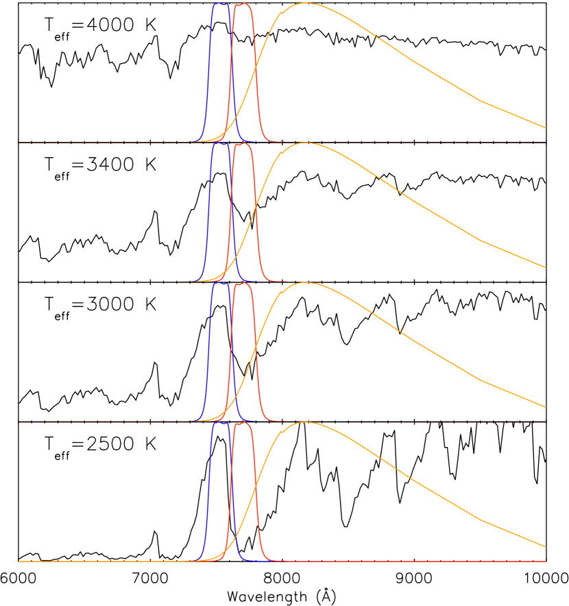
Figure 1.— The band profiles of the 3 WFI filters used in this work (from left to right: 753, 770 and $I-band$) overlaid to spectra of very low-mass stars (4000 K to 3000 K) and BDs (3000 K to 2500 K) from Allard et al. (2000).

Table 1Characteristics of the filters used for our WFI imaging

band	$\lambda$ central	FWHM	E.W.	Vega zero-point
	($\AA$)	($\AA$)	($\AA$)	(erg s-1 cm-2 $\AA^{-1}$)
753	7536.2	184.1	191.4	1.368$\cdot 10^{-9}$
770	7707.9	195.2	201.3	1.275$\cdot 10^{-9}$
I	8620.5	1354.9	1431.2	9.500$\cdot 10^{-10}$

The WFI imaging was carried out during 5 nights of December 2010. On each night, observations were performed in all the three bands together so as to minimize the impact of any longer timescale stellar variability. A standard dithering pattern has been applied, in order to cover the gaps between the 8 CCD chips of WFI and allow for cosmic ray and bad pixel removal. We did not carry out short exposures to avoid saturation for the bright sources, since the bright end of the ONC has been studied well in detail by us in our previous works. Dark, bias and flat field exposures were obtained before and after each night. We did not observe standard fields for photometric calibration, given the particular filters used in this program and the practicality of performing relative photometric calibration exploiting our large pre-existing data set on Orion.

Table 2WFI observations

band	exposure time	n. of exposures	total exposure time
	($s$)		(s)
753	360	23	9,360
770	500	28	14,000
$I$	280	12	3,360

2.2. Data reduction

Images were processed using the ESO/MVM (Multi-Vision Model) vers. 1.3.5 package (Vandame, 2004). This software automatically performs all common image reduction steps (e.g., correction for bias and flat fields), and the absolute astrometric calibration of the individual exposures to be merged. This is accomplished by cross-correlating the images with a reference astrometric catalog; we utilized to this purpose our previous WFI photometric catalog presented in Paper I. The final product of our image reduction is 3 images, one for each filter, obtained by merging all the individual exposures. Table 2 summarizes the total exposures times; these about 1 hour for the broad band, and about 2.5 and 4 hours for the two medium bands,

Photometry, both aperture and point-spread-function (PSF), was performed using the Daophot II package (Stetson, 1987). We computed the PSF individually for every image, starting from a coadded sample of few hundreds bright and unsaturated sources, and then refining these with an iterative sigma-clipping method to reject PSF stars with poor $\chi^{2}$. Photometry was computed on all the sources brighter than 3$\sigma$ above the local sky background noise. In order to eliminate the contamination from spurious detections—a potentially significant fraction of the total detections, given the strong variability of the nebular background, and the low threshold for source detection—we rejected sources not present in any of our existing deep photometric catalogs of the ONC, both ground based (WFI $UBVI$, Paper I; CTIO/ISPI $JHK$, see Robberto et al. 2010) or from the HST photometry (ACS $BVIZ$, WFPC2 $UBI$, see Robberto et al. 2005). In particular, the significant depth of the infrared and HST data, over a FOV equal or larger than that of the observations described here, guarantees that we are not excluding any real sources in this study.

The photometry has been calibrated to the VegaMag system using our previous WFI photometric catalog. For the $I$-band, we simply determined the photometric offset with respect to our previous photometry in the same filter. For the two medium bands, we used synthetic photometry. We considered the atmosphere models of Allard et al. (2000) as empirically calibrated by us in Paper II, and computed the two medium-band colors $(MB-I)$ as a function of $T_{\rm eff}$. Then we considered the actual sources detected in all 3 bands and for which we have $T_{\rm eff}$ and $A_{V}$ from Paper II, and plotted the measured, extinction-corrected ($MB_{\rm instrumental}-I_{calibrated}$) colors against $T_{\rm eff}$. The systematic difference between these colors (considered individually) and the synthetic ones is the offset needed to calibrate the medium bands. Specifically, we limited to the stars with $T_{\rm eff}>4000$ K, range where the possible inaccuracies of the atmosphere models are very modest.

2.3. Completeness

Figure 2.— Photometric completeness functions for our three filters.

We derive the completeness functions for our WFI photometry with an artificial star test, performed separately for each WFI filter. Artificial stars of different magnitude, are added on the reduced WFI images; then, with the same technique used to detect and extract photometry on the real stars, these artificial stars are recovered or missed depending on their flux, local sky noise, crowding, etc. The fraction of recovered stars against the total, as a function of magnitude, provides the completeness.

In our ONC imaging, the completeness is spatially variable, being strongly affected by the nebular background, which is brighter at the center where the stellar density is higher. This correlation, if not accounted for, may bias the derived completeness. Therefore, we first derive the spatial, projected, stellar density distribution of the ONC. This is obtained by merging all catalogs at our disposal, in particular the deep ISPI $JHK$ photometry and the HST/ACS data. Then, for every magnitude bin, the artificial stars are generated with random positions drawn from the 2 dimensional density distribution.

The derived completeness functions are shown in Figure 2. In all cases, these curves show a characteristic trend: besides the typical steep cutoff at faint luminosities which traces the detection limit, the completeness shows a slow decrease below 1 at bright luminosities. This is due to the luminous nebular emission and significant crowding of the central part of the ONC, where the detection limit is significantly poorer. In the outer regions of the ONC, we are able to detect sources all the way down to $m\sim 22.5$ mag in $I$ band (see Figure 4), and to $m\sim 23.5$ mag in $753$ and $770$.

2.4. Photometry results

Figure 3.— Photometric errors as a function of magnitude, for the 3 photometric bands

Figure 4.— Open circles: the derived $I$ vs $753-I$ CMD including only the sources measured in all the 3 bands (i.e. also in $770$). The filled blue circles indicate the sources included in our previous study of the stellar population of the ONC, based on WFI photometry and spectroscopy down to the H-burning limit (Paper II). The average photometric errors as a function of $I$-band are indicated to the right. The red line represents a 1 Myr Baraffe et al. (1998) isochrone; the square, circle and triangle symbols along the line mark masses of 0.4 M_⊙, 0.08 M_⊙ and 0.02 M_⊙. The arrow denotes the reddening vector for $A_{V}=2$ assuming the Cardelli et al. (1989) reddening law for $R_{V}=3.1$.

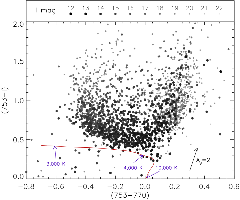
Figure 5.— $(753-I)$ vs. $(753-770)$ color-color diagram from our photometry. The color and size of the dots indicates the I-band luminosity of each source, as indicated. The black arrow indicates the direction of the reddening vector for 2 mag of extinction in $V-$band, assuming the reddening law of Cardelli et al. (1989) for $R_{V}=3.1$. For reference, the thick red line is the empirical isochrone derived in Paper II converted in this color-color plane using the atmosphere models of Allard et al. (2000). For guidance, the origin (0,0) corresponds to 10,000 K, and the turn-over in $(753-770)$ corresponds to $T_{\rm eff}\sim 4000$ K, i.e. between K and M spectral classes.

The final catalog includes 2474 sources with photometry in all 3 bands. The photometric errors as a function of magnitude are shown in Figure 3. Figure 4 shows our new CMD, highlighting the significant improvement in depth with respect to our previous work (Paper II). In particular, our photometry covers a very large range of stellar luminosities, spanning $\sim 9$ mag in $I$-band, and the new observations extend $\sim$5 mag deeper than in the previous work, reaching $I\simeq 22$, which corresponds to young sources with masses $<0.02$ M_⊙ at 1 Myr (see Figure 4). In Figure 4 we also observe among the faintest sources a concentration of objects with $I\gtrsim 18$ which, as we show below, comprise a distant, background stellar population that is detectable despite the high extinction through the molecular cloud because of the depth of our observations.

In Figure 5 we present the $(753-I)$ vs $(753-770)$ color-color diagram, which forms the basis of our analysis in all that follows. The most salient feature of this diagram is the inflection point near (0.05,0.25), from which the stars extend in two different directions. By comparison with the orientations of the synthetic isochrone and the extinction vector, we see that this inflection in the diagram essentially separates the stars into a group (extending to the left) that stretches mostly parallel to the isochrone and perpendicular to the reddening vector, and a second group (extending to the upper right) that stretches parallel to both the isochrone and the reddening vector. The inflection in the diagram occurs at $T_{\rm eff}\approx 4000$ K.

For stars with $T_{\rm eff}\lesssim 4000$ K (i.e. spectral types $>$M0), the $(753-770)$ color is both highly sensitive to $T_{\rm eff}$, becoming rapidly bluer (more negative) as $T_{\rm eff}$ decreases (see also Figure 1), and largely insensitive to $A_{V}$ because of the small wavelength separation between the 753 and 770 bands. In our analysis below we exploit this property of the diagram to break the degeneracy between $T_{\rm eff}$ and $A_{V}$ for these very cool stars, which has previously been one of the most difficult challenges in the derivation of stellar parameters from optical broadband photometry for M-stars and BDs (Hillenbrand 1997; Paper II). We note here that the synthetic isochrone clearly does not correctly reproduce the slight upward curvature of the stars as one moves to the coolest $T_{\rm eff}$, but because these cool stars nonetheless extend perpendicular to the reddening vector, we demonstrate below that the systematic error in the $(753-I)$ colors predicted by the synthetic isochrones can be readily calibrated out for $T_{\rm eff}\lesssim 4000$ K. We note also that the effects of contamination by faint background sources is mitigated in this region of the diagram, particularly for the coolest objects of interest ($T_{\rm eff}\lesssim 2900$ K, i.e., in the BDs regime), since background BDs are too intrinsically faint to penetrate the very high $A_{V}$ of the cloud behind the ONC. As we show in Section 4, the relatively few remaining background contaminants in this region of the diagram (mostly red giants) can be filtered out on the basis of their luminosity.

These desirable features of the $(753-I)$ vs $(753-770)$ color-color diagram break down for warmer stars with $T_{\rm eff}>5000$ K. For these warmer stars the colors are largely degenerate in $T_{\rm eff}$ and moreover the isochrone and the reddening vector are parallel. For these stars we must therefore rely on previous observations by us and from the literature to determine $T_{\rm eff}$ and $A_{V}$. In addition, there is significant background contamination in this region of the diagram; as we show below, while the brightest of these stars are bona fide ONC members, the faintest are mostly background stars. Finally, we note that the apparent lack of low-$A_{V}$ stars for $T_{\rm eff}\gtrsim 4000$ K is the result of these stars being saturated in our deep images. Such stars are indeed present in the ONC, and we include them in our analysis from our own previous work (Paper I and II).

3. Analysis

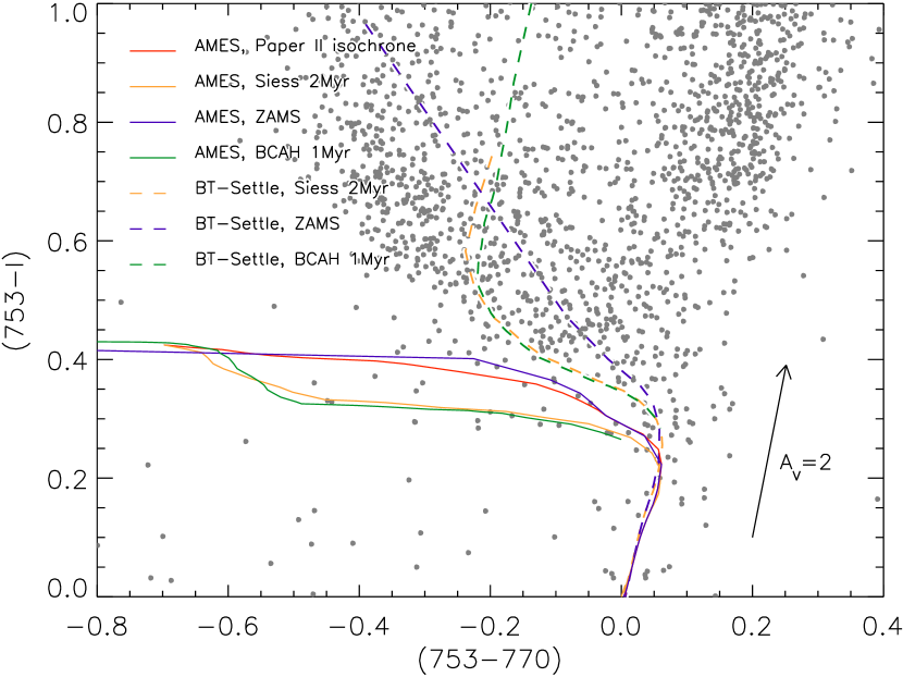
Figure 6.— The color-color diagram of Figure 5, with different synthetic isochrones overplotted. In particular: a Siess et al. (2000) 2 Myr isochrone; a Baraffe et al. (1998) 1 Myr isochrone; a Siess et al. (2000) zero-age main sequence. Thick lines are the result from synthetic photometry on the AMES-MT grid of spectra from Allard et al. (2000), while dashed line are computed using the BT-Settle grid from Allard et al. (2010). The thick red line is computed using the empirical calibration of the AMES-MT models defined in our Paper II to match the broad band $BVI$ colors of the ONC. The empirical line is actually closer to the predicted ZAMS relation than the predicted 1-2 Myr isochrones, illustrating the current lack of agreement between evolutionary and atmosphere models and young star photometry (see text).

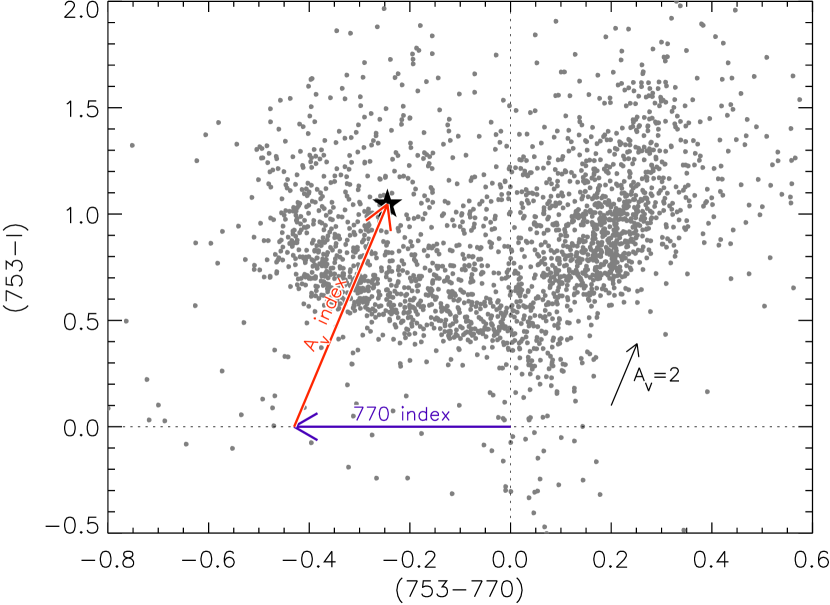
Figure 7.— Conceptual scheme of the new coordinate system we introduce to measure $T_{\rm eff}$ and $A_{V}$ of the stars from our color-color diagram: the $T_{\rm eff}$ dependent [$770~{}index$], and the reddening dependent $A_{V}$ index. See text.

In order to derive the stellar parameters of very low-mass stars (VLMSs) and BDs in the ONC, we focus our analysis on the left-hand part of the color-color diagram of Figure 5, where the $(753-770)$ color anti-correlates with $T_{\rm eff}$.

Our basic methodology is to project each source from its observed position in the color-color diagram back along the reddening vector to the theoretical isochrone. The choice of theoretical isochrone is largely arbitrary because none of the available isochrones exactly reproduce the observed distribution of the stars in the diagram, and consequently we must empirically recalibrate the isochrone based on the observed distribution. Our assumption is that, whichever fiducial isochrone is adopted, the non-reddened stars should lie on the isochrone, and the reddened stars displaced away from it along the reddening vector. For example, the isochrone shown in Figure 5 computed using the synthetic spectra of Allard et al. (2000) predicts a much bluer $(753-I)$ index than our data for low $(753-770)$. If the model were correct, this would imply an unrealistic dependence of the average $A_{V}$ on $T_{\rm eff}$, in the sense that the minimum measured extinction (i.e. the distance, along the reddening vector, between the isochrone and the stars) increases monotonically with decreasing $T_{\rm eff}$.

Different synthetic isochrones can lead to more realistic predictions of colors. Figure 6 shows our color-color diagram with a number of synthetic isochrones, computed using both the AMES-MT spectra of Allard et al. (2000) and the most recent grid—the BT-Settle models—from Allard et al. (2010). We also show an isochrone (red line) derived using the Allard et al. (2000) atmospheres as recalibrated by us in Paper II. That calibration, appropriate for the ONC, involved an empirical constraint on the stellar $\log g$ to produce a synthetic isochrone that matched the observed broadband colors of the ONC in $BVI$. It is clear that all synthetic isochrones, including that which we used in Paper II, are incompatible with the data in this new medium-band color-color plane. AMES-MT consistently predicts a systematically lower $(753-I)$ at low $T_{\rm eff}$, and BT-Settle predicts either a turn-over in $(753-770)$ for low $\log g$ (young isochrones) or $(753-I)$ colors that are too red for high $\log g$ (the ZAMS model). Evidently, current synthetic models, even those that have been empirically calibrated by us to match the broadband colors of young low-mass stars, are unable to correctly reproduce the molecular feature at $\lambda\sim 7700$Å and/or the photospheric continuum level at $\lambda\sim 7500$Å which form the basis of our new medium-band color-color diagram technique. As a consequence, we must empirically define an isochrone representing both the photospheric colors in our bands and the $T_{\rm eff}$ scale along it.

To proceed, we introduce a new set of coordinates in the color-color plane of Figure 5. We define the $[A_{V}~{}index]$ as the distance that a given star is displaced, along the reddening vector, from the $x-$axis of the color-color diagram, measured in units of $A_{V}$:

$$[A_{V}~{}index]= \bigg{(}m_{753}-I\bigg{)}\bigg{/}\bigg{(}\frac{A_{753}}{A_{V}}-\frac{A_{I}}{A_{V}}\bigg{)}$$ (1)

where $A_{753}/A_{V}=0.678$, $A_{770}/A_{V}=0.652$ and $A_{I}/A_{V}=0.533$ (values computed from the Cardelli et al. (1989) reddening law for $R_{V}=3.1$). We choose the reddening parameter $R_{V}=3.1$ instead of a higher value (e.g, 5.5, Costero & Peimbert 1970) because, as we found in Paper II, this value better explains the observed broadband colors of the ONC members. We similarly define the $[770~{}index]$ as the projection of a given star, along the direction of the reddening vector, onto the x-axis [i.e. $(753-I)=0$]:

$$[770~{}index]= m_{753}\cdot\bigg{[}1-\big{(}\frac{A_{753}}{A_{V}}-\frac{A_{770}}{A_{V}}\big{)}/\big{(}\frac{A_{753}}{A_{V}}-\frac{A_{I}}{A_{V}}\big{)}\bigg{]}+$$ (2)

$$+I\cdot\bigg{[}\big{(}\frac{A_{753}}{A_{V}}-\frac{A_{770}}{A_{V}}\big{)}/\big{(}\frac{A_{753}}{A_{V}}-\frac{A_{I}}{A_{V}}\big{)}\bigg{]}+$$

$$-m_{770}$$

By definition, the $[770~{}index]$ is reddening independent, and so it depends only on $T_{\rm eff}$. Figure 7 shows a schematic representation of the two indices in the color-color diagram.

3.1. Derivation of $T_{\rm eff}$

Because the currently available synthetic spectra are unable to accurately predict the stellar colors in our medium-band color-color diagram, we must derive an empirical transformation between the $[770~{}index]$ and $T_{\rm eff}$. To this end we utilize the sample of ONC stars with directly determined (i.e. spectroscopic) spectral types. With the appropriate transformation between the $[770~{}index]$ and $T_{\rm eff}$, we will be able to reliably determine $T_{\rm eff}$ of all the other members from their measured [$770~{}index$]. We have assembled all available optical spectral types from our Paper II (for stellar-mass objects) and NIR spectral types (for substellar-mass objects) from Riddick et al. (2007) and Slesnick et al. (2004). The spectral types were converted to $T_{\rm eff}$ using the temperature scale of Luhman et al. (2000), as we did in Paper II.

Figure 8 shows the resulting relationship between our measured [$770~{}index$] and the spectroscopically determined $T_{\rm eff}$. As expected, for late spectral subtypes the $[770~{}index]$ becomes bluer (i.e. becomes more negative) with $T_{\rm eff}$. This approximately linear dependence holds from $T_{\rm eff}\sim 3500$ K ($\sim$M2.5) down to the coldest available spectral types for BDs, and down to our photometric lower limit ($[770~{}index]\simeq 0.8$).

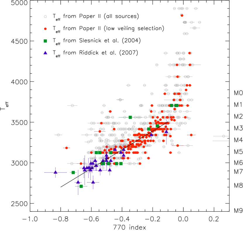
Figure 8.— Derived relation between the measured, reddening independent, photometric $[770~{}index]$, and spectroscopically determined stellar temperature. The values of $T_{\rm eff}$ for the stellar mass regime ($T_{\rm eff}\gtrsim 3000$ K) are from the spectral types collected in our Paper II. For these sources, we identify a sample of candidate weak accretors, showing low H$\alpha$ emission (E.W.$<10\AA$) and no significant veiling ($\log L_{\rm accr}/L_{\rm tot}<-1.5$), in order to more cleanly determine the true relationship between the photometric $[770~{}index]$ and $T_{\rm eff}$. Spectroscopic $T_{\rm eff}$ for substellar masses are from Riddick et al. (2007) and Slesnick et al. (2004). See text for details.

Perhaps not surprisingly, we found that the scatter in the [$770~{}index$]–$T_{\rm eff}$ relation could be significantly reduced if we consider only sources that do not show strong spectroscopic evidence of accretion. We selected the “non-accretors” on the basis of low H$\alpha$ emission (E.W.$<10\AA$) from Paper I and low optical veiling (low $B-$band excess emission) from Paper II. Figure 8 shows that these non-accretors form a relatively tight sequence, while the rest of the stars (the accretors) are much more scattered in the diagram. The accretors are also systematically shifted to higher $T_{\rm eff}$ and/or lower [$770~{}index$], indicating that accretion alters the position of the sources in the diagram, and indeed below we exploit this feature to quantify the degree to which accretion may affect our determination of $T_{\rm eff}$.

Using only the sample of non-accretors, we derive an empirical linear relation between $T_{\rm eff}$ and the $[770~{}index]$:

$$T_{\rm eff}=3620~{}{\rm K}+[770~{}index]\cdot 1150~{}{\rm K}$$ (3)

which is valid for $[770~{}index]<-0.1$. The standard deviation of the data relative to this relation is $\sim 100$ K, roughly corresponding to one-half of a spectral subtype. This is comparable to the overall uncertainty in our spectroscopically determined $T_{\rm eff}$ from Paper II, suggesting that this scatter is principally due to uncertainty in the (spectroscopic) spectral types, and therefore any additional uncertainty introduced through the $[770~{}index]$–$T_{\rm eff}$ transformation is negligible.

3.2. Influence of accretion excess on the $T_{\rm eff}$ estimation.

The analysis methodology utilizing our medium-band color-color diagram is predicated on the assumption that the stellar colors in our photometric bands depend only on $T_{\rm eff}$ and $A_{V}$, permitting us to establish an empirical relationship between the our [$770~{}index$] and $T_{\rm eff}$ (Equation 3). However, the colors of young stars can be affected by accretion, whereby infalling matter from the circumstellar disk onto the stellar surface leads to a flux excess, strongest in the UV and in specific emission lines, but also to a smaller extent in the continuum at optical wavelengths. The latter is typically characterized by a heated photosphere covering $\sim$1% of the stellar surface and with $T_{\rm eff}\sim 6000-8000$ K, therefore peaking in the B-band (Calvet & Gullbring, 1998). Since our photometry uses filters at the red end of the optical spectrum, and there are no emission lines within the wavelength range covered by our filters, we expect that accretion should induce only a modest alteration of our measured colors.

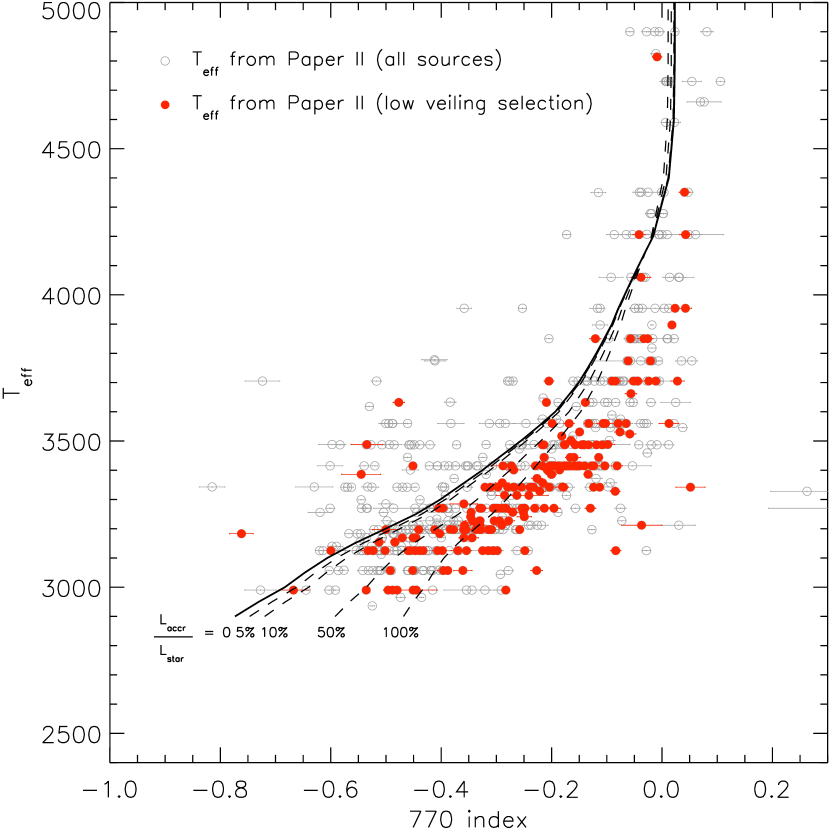
Figure 9.— Same as Figure 8, showing the displacement in the reddening-independent $[770~{}index]$ obtained by adding an amount of accretion luminosity to the star. The thick line is the isochrone from Paper II, the same model shown also in Figure 5. The dashed line are the same model, after the addition of a given amount of accretion luminosity to the each synthetic spectrum, for different values of $\log L_{\rm accr}/L_{\rm tot}.$ Note that the fact that the red dots are low accretion sources, whereas the model requires a large value of $L_{\rm accr}$ to predict their colors, implies that the base isochrone needs adjustments (see text).

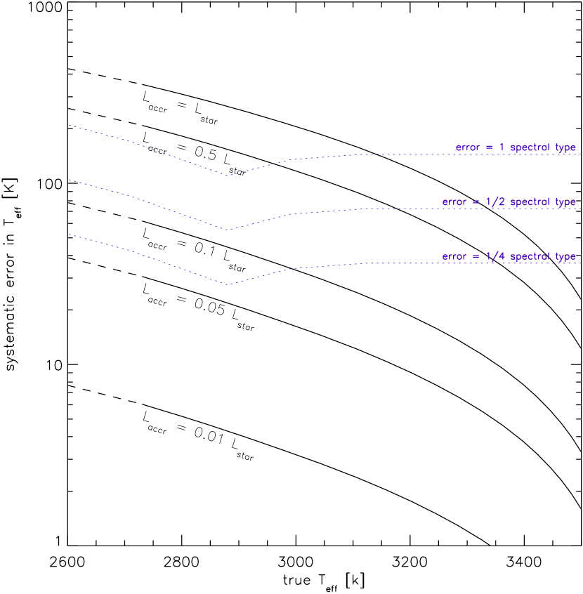
Figure 10.— Computation of the offset on the derived $T_{\rm eff}$, as a function of temperature, produced by neglecting accretion veiling. The solid lines represent the result for different accretion luminosities. The dotted lines represent the uncertainty in $T_{\rm eff}$ associated to un uncertainty in the spectral type of 1 subtype, half subtype and 1/4 of a subtype.

We investigate this hypothesis in a quantitative way, calculating the shift in [$770~{}index$], at constant $T_{\rm eff}$, obtained by contaminating the photospheric fluxes with varying degrees of accretion luminosity. As in Paper II, where we performed a similar modeling to derive the change in the $BVI$ colors due to mass accretion, we first model a typical accretion spectrum, then we add it with increasing relative flux fraction on synthetic stellar spectra of different $T_{\rm eff}$. Finally, by means of synthetic photometry as above, we compute the resulting changes in the $[770~{}index]$ and in turn the error induced in the inferred $T_{\rm eff}$. Specifically, we simulated a typical accretion spectrum using the Cloudy photoionization code. This is similar to that we used in Paper II, but has been further refined to provide a more realistic SED in the ultraviolet range (Manara et al. 2011, in prep.). We use the synthetic spectra that we used in Paper II–namely the empirically calibrated AMES-MT model from Allard et al. (2000)—and for every $T_{\rm eff}$ we add a component of our accretion spectrum to the photospheric spectra, varying the ratio $L_{\rm accr}/L_{\rm star}$.

The result is shown in Figure 9, from which two main results are evident: First, contaminating the stellar flux with accretion excess shifts the [$770~{}index$] to higher values, and the effect is more prominent for cooler $T_{\rm eff}$. This is intuitive considering that this index traces the ratio between the flux outside ($\lambda\sim 7530$Å) and inside ($\lambda\sim 7700$Å) the TiO molecular feature. The accretion-induced continuum excess partially “fills in” the TiO absorption feature, leading to higher (less negative) values of [$770~{}index$]. Second, for typical values of accretion luminosities in a PMS cluster ($L_{\rm accr}\lesssim L_{\rm star}$) the shift in the [$770~{}index$] is negligible.

From Figure 9 it also appears that the synthetic isochrone does not quite follow our data. This is not surprising, given that, as discussed in Section 2, this model provides a somewhat inaccurate estimate of the stellar fluxes in our medium bands (see Figure 6). Therefore, in order to obtain a correct, quantitative assessment of the accretion-induced shift in the [$770~{}index$], we must recalibrate the results shown in Figure 9. We proceed as follows. The systematic error in the depth of the TiO feature as a function of $T_{\rm eff}$ can be treated as a simple systematic error in the $T_{\rm eff}$ scale. For example, for the lowest $T_{\rm eff}$ modeled in Figure 9 ($T_{\rm eff}\simeq 2950$ K), the models predict a depth of the TiO feature corresponding to [$770~{}index$]$=-0.8$ mag, and by adding $10\%$ of accretion luminosity one obtains a shift of the index of $\sim 0.06$ mag. In fact, from Figure 8 and Equation 3, [$770~{}index$]$=-0.8$ mag corresponds to a lower $T_{\rm eff}$, about 2700 K. Therefore we can associate this $T_{\rm eff}$ with a shift of $\sim 0.06$ mag. Then, we readjust the ratio $L_{\rm accr}/L_{\rm star}$, using the updated $T_{\rm eff}$, according to $L_{\rm star}\propto T_{\rm eff}^{4}$.

Finally, we can recast the result from a more observational perspective, in which we measure [$770~{}index$] for a given star and we do not know the true value of $L_{\rm accr}$ for that star. Deriving $T_{\rm eff}$ via Equation 3, which is defined for $L_{\rm accr}=0$, we will overestimate the true $T_{\rm eff}$ because accretion will cause the TiO feature to be filled-in and consequently we will measure a higher [$770-index$]. Figure 10 shows the resulting systematic overestimation of the derived $T_{\rm eff}$ for various $L_{\rm accr}$. We find again that the lower the stellar $T_{\rm eff}$, the larger the error in the $T_{\rm eff}$ estimate due to accretion. However, if one excludes very strong accretors ($L_{\rm accr}\simeq L_{\rm star}$), the error in $T_{\rm eff}$ is very small. For instance, for $L_{\rm accr}=10\%L_{\rm star}$, the $T_{\rm eff}$ error is always smaller than half spectral subtype, and always $<40$ K above the H-burning limit ($T_{\rm eff}\sim 3000$ K). The $T_{\rm eff}$ difference associated to an error of 1 spectral type was computed as the difference between the temperature of two contiguous spectral subtypes. Similarly, the $T_{\rm eff}$ differences corresponding to $1/2$ and $1/4$ spectral subtypes (dotted lines in Figure 10) is equal to that for 1 spectral type, scaled down by a factor of 2 and 4.

In conclusion, the presence of optical excess due to accretion has a negligible effect on the stellar parameters derived from our medium-band survey. Thus, we will neglect accretion in the following analysis, and proceed to derive $T_{\rm eff}$ based on the [$770~{}index$] from Equation 3.

3.3. Accuracy of $T_{\rm eff}$ from previous works

Despite having shown that accretion excess not not alter significantly the measured [$770~{}index$], Figure 8 showed that accreting ONC sources are displaced in the $T_{\rm eff}$ vs. [$770~{}index$] plane. The displacement is such that the accretors lie above the non-accretors, meaning that the spectroscopic $T_{\rm eff}$ plotted on the y-axis of Figure 8 have been on average overestimated for accreting ONC sources.

This overestimation of spectroscopically determined $T_{\rm eff}$ for accreting sources is likely the result of incomplete removal of the optical veiling in the spectra of these sources. This excess, that we demonstrated above to be minimized at 7700Å(although it may still be present in extreme cases, see, e.g., Fischer et al. 2011), is likely larger at bluer wavelengths, where other molecular features are typically used to measure the spectral types of M-type stars. This veiling, if not removed or if incompletely removed, will fill in the molecular absorption lines and lead to a systematic overestimation of the spectral types.

By utilizing the [$770~{}index$] to derive $T_{\rm eff}$ we are instead largely immune to these effects, and we are now able to correct the previous spectroscopically derived $T_{\rm eff}$ via equation Equation 3.

In conclusion, our technique to measure stellar $T_{\rm eff}$ is able to derive a more accurate estimate of $T_{\rm eff}$ than optical spectroscopy, being less biased by a possible veiling excess.

3.4. Calibration of the [$A_{V}~{}index$] and derivation of extinctions

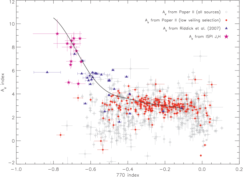
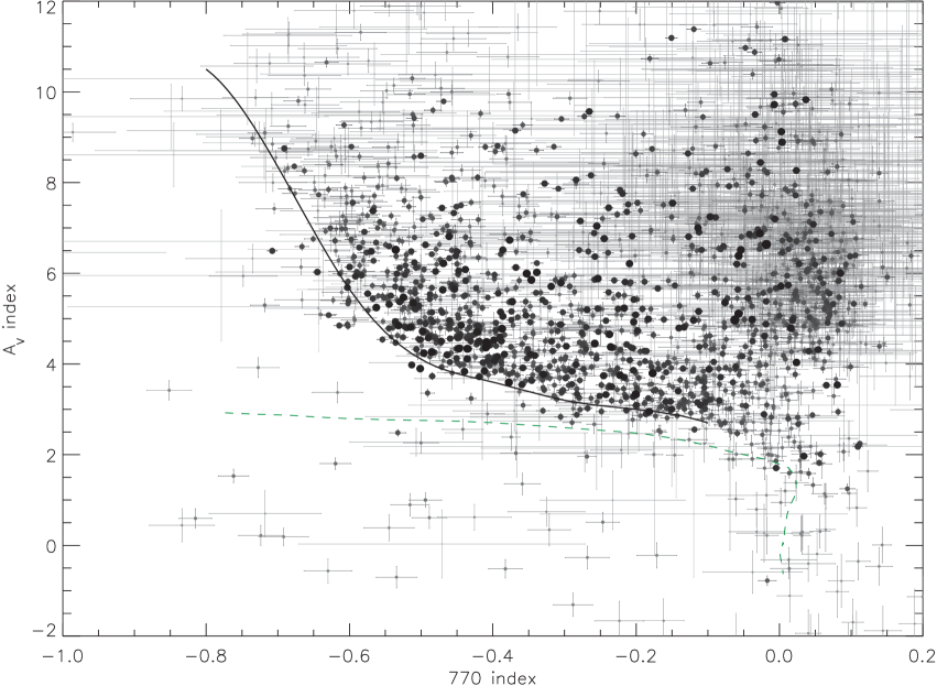
Figure 11.— The color-color plot expressed in units of $[770~{}index]$ (reddening independent) and $[A_{V}~{}index]$ (parallel to the reddening direction). Left panel: sample of extinction-corrected sources; $A_{V}$ values are from Riddick et al. (2007), the $JHK$ photometry of Robberto et al. (2010), and the optical analysis of Paper II. For the latter, accretors and candidate non accretors are distinguished as in Figure 8. The solid line represents our best fit of the data, i.e. the empirical isochrone for $A_{V}=0$. Right panel: same diagram, reporting all the sources in our catalog, with no correction for extinction. These are color coded according to their photometric errors. The entire population, with the exception of very few sparse sources, is located above the isochrone, at positive values of extinction.

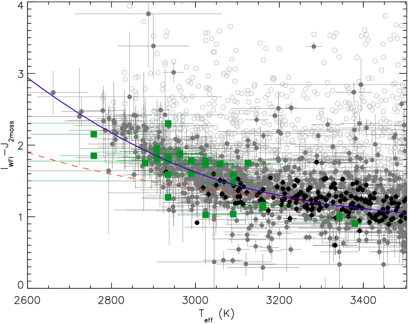
Figure 12.— $(I-J)$ vs $T_{\rm eff}$: the open dots are the measured colors, the filled gray dots are the de-reddened ones. Black dots are dereddened colors for sources with know estimate of accretion excess, showing no significant excess. Green squares are sources whose $T_{\rm eff}$ is from Riddick et al. (2007). The dashed line is the prediction from synthetic photometry on the BT-Settle atmosphere models of Allard et al. (2010); the solid line is the empirical fit to the data.

In section 3.1 we derived an empirical relation between the $[770~{}index]$ and the stellar $T_{\rm eff}$, and in section 3.2 we explored the effects of accretion luminosity on there derivations. Here, similarly, we find the relation between the $[A_{V}~{}index]$, obtained in Equation 1, and the actual extinction $A_{V}$ of the ONC stars, in magnitudes. In the color-color diagram, the extinction $A_{V}$ of a star is the distance, along the reddening direction, between the observed position and the isochrone, whereas the [$A_{V}~{}index$] is the distance, also along the same direction and scaled by the appropriate $A_{\lambda}/A_{V}$, between the observed colors and the abscissa $(770-753)=0$. Therefore the [$A_{V}-index$] and the true $A_{V}$ differ only by a constant, which depends on the [$770~{}index$] (i.e., it is a function of $T_{\rm eff}$).

To this end, we plot the extinction-corrected ONC stars with independent $A_{V}$ estimates from Paper II and from Riddick et al. (2007) in the [$A_{V}~{}index$] vs. [$770~{}index$] plane (Figure 11, left-hand panel). We also use the ISPI $JHK$ photometry of the ONC presented in Robberto et al. (2010), from which we use stars with the lowest $T_{\rm eff}$ (low $[770~{}index]$) and with the smallest photometric errors. For the coolest $T_{\rm eff}$ considered here, the $J$ vs $(J-H)$ isochrone from Robberto et al. (2010) is vertical, and its color ($J-H\simeq 0.65$) is independent of age, therefore $A_{V}$ can be derived by simply dereddening the sources on the isochrone. By not including the $K$-band photometry from Robberto et al. (2010), the infrared-derived extinctions should not be strongly affected by the possible presence of disk excess. The thick line in the figure is our fit to the data, i.e., the empirical isochrone corresponding to $A_{V}$=0. This also represents the offset to be subtracted from the measured $[A_{V}~{}index]$, as a function of the [$770~{}index$], to compute the true $A_{V}$.

Among the points in Figure 11 from our previous Paper II, we can distinguish accreting sources from non-accretors, just as in Figure 8. In Section 3.1 we suggested that previous spectroscopically derived $T_{\rm eff}$ estimates are systematically overestimated for accreting members in the M-type range. This is now confirmed by Figure 11: whereas the extinction-corrected non-accretors lie on a curve consistent with the lower edge of the non extinction-corrected population (right panel of the same Figure), for accretors we find $A_{V}$ estimates systematically overestimated. This is because if $T_{\rm eff}$ is overestimated, the intrinsic colors are underestimated, and therefore the color excess attributed to extinction is overestimated leading to higher $A_{V}$.

Figure 11, right-hand panel, shows again the empirically calibrated isochrone (i.e., for $A_{V}=0$), together with all the stars in our catalog. Unlike in the left-hand panel, we have not subtracted the extinction here. Overall the population lies above the line, i.e., at positive values of $A_{V}$. As would be expected if the isochrone is correct, the distribution of sources above the isochrone also appears uniform for different $[770~{}index]$. There is an overabundance of highly reddened stars at the highest useful limit of the index ($[770~{}index]=-0.1$), i.e., at the highest limit of the $T_{\rm eff}$ range accessible with our medium-band photometry. This, as will be shown below, is a residual late-type background contaminant population.

4. The H-R diagram

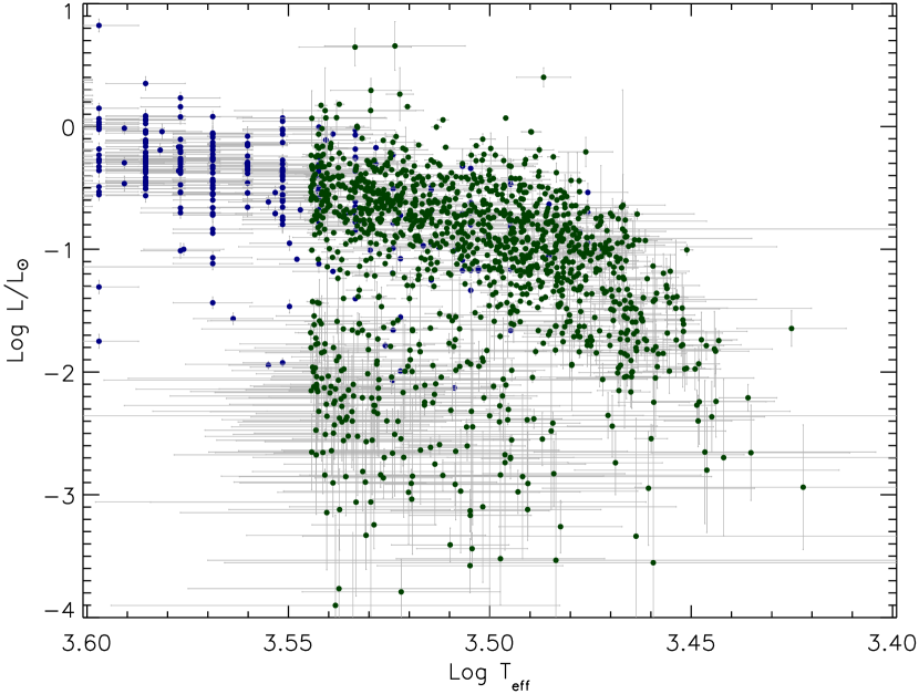
Figure 13.— The new H-R diagram of the ONC. Green dots are the new stars whose stellar parameters have been derived in this work, blue dots are members from Paper II, mostly having a large enough $T_{\rm eff}$ to not be derivable using the $[770~{}index]$, or saturated in our new WFI photometry.

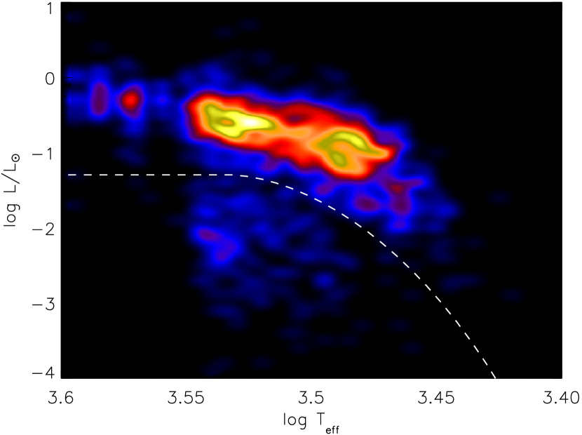
Figure 14.— Stellar density map in the H-R diagram. The dashed line marks our adopted separation between bona fide members and contaminants.

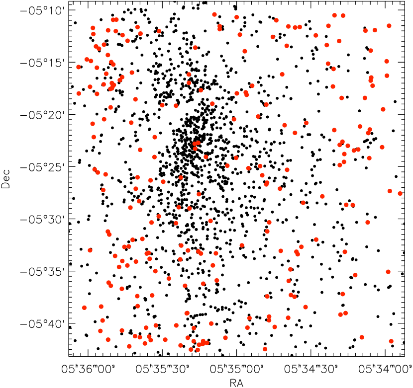
Figure 15.— Spatial distribution of the ONC members placed in the H-R diagram (black dots). The red circles mark the position of the faint sources identified as background sources.

Having derived two empirical relations, one to obtain the $T_{\rm eff}$ from the $[770~{}index]$ for stars in the spectral subtype range M3–M8.5, the other to derive $A_{V}$ once the $[770~{}index]$ is known, we now derive the stellar parameters for the sources in our catalog.

Sources lying below the isochrone of Figure 11b appear to have negative extinctions, which is unphysical; 93 stars showing an extinction in the range $-2$ mag$<A_{V}<$0 mag are therefore assigned $A_{V}=0$, essentially shifting the measured colors to the closest physically meaningful solution. Another few stars with $A_{V}<-2$ mag were removed from the sample, being likely spurious detections or faint sources with very inaccurate photometry. The fraction of sources showing negative extinction (about 5%) is much smaller than in previous works (e.g., Paper II or Hillenbrand 1997), validating the improved accuracy of our methods to derive stellar parameters. In total, we derived $T_{\rm eff}$ and $A_{V}$ for 1280 sources, whereas only 544 of them had a previously assigned $T_{\rm eff}$. Merging the new $T_{\rm eff}$ and $A_{V}$ with those of our previous work, our sample counts 1807 sources with both $T_{\rm eff}$ and $A_{V}$ from which we can derive an updated H-R diagram for the ONC extending to well below the H-burning limit.

4.1. Bolometric corrections

In order to convert the de-reddened magnitudes into $\log L/L_{\odot}$, knowledge of the bolometric corrections (BCs) as a function of $T_{\rm eff}$ is required. Unfortunately, we cannot rely for such relations on previous works (e.g., Flower, 1996; Bessell et al., 1998) for several reasons: 1) the photometric bands used here, including $I-$band, are non-standard; 2) optical BCs usually do not extend in the BD temperature range; and 3) if the optical stellar colors are age dependent, as suggested in Paper II, the BCs may be also. Thus, BCs valid for main-sequence dwarfs might not be adequate for a young populations such as the ONC. Instead, we use synthetic photometry to derive our BCs, according to the formula:

$${\rm BC}=2.5\cdot\log\bigg{[}\frac{\int f_{\lambda}(T)\cdot S_{\lambda}d\lambda}{\int f_{\lambda}(T)\cdot d\lambda}\bigg{/}\frac{\int f_{\lambda}(\odot)\cdot S_{\lambda}d\lambda}{\int f_{\lambda}(\odot)\cdot d\lambda}\bigg{]},$$ (4)

where $f_{\lambda}(T)$ are synthetic spectra, and $S_{\lambda}$ the filter throughput.

As we have shown above (see also the discussion in Paper II), current atmosphere models do not correctly predict the optical broad band colors for cool stars. This clearly affects the computation of BCs, in particular BCs in $I-$band, $BC_{I}$. On the other hand, the bolometric flux for a given synthetic spectrum will be trivially correct at a given $T_{\rm eff}$ since, by definition, $L\propto R^{2}T^{4}$. The radii $R$, which could also be inaccurate from the evolutionary models, do not affect the BCs since they introduce an identical proportionality factor in both the numerator and denominator of equation 4.

From the comparison of our data with the synthetic isochrones (see Figure 6) we cannot ascertain the correctness of the synthetic $I$-band fluxes. It is true that the isochrones are unable to reproduce the data in the color-color diagram, but the shortcomings may be principally in our medium bands and not in the $I$-band. At the same time, the BT-Settle models (Allard et al., 2010) have been validated in the NIR for dwarf stars, such that the predicted $J$ and $K$ fluxes match the observations down to BD masses. Thus, if the predicted $I-$band magnitudes are also correct, we would expect the predicted $(I-J)$ color to be also consistent with the observations across all $T_{\rm eff}$.

We perform this test using the $J$-band photometry of the ONC from Robberto et al. (2010), together with our $I-$band magnitudes and (as in Section 3.4) the $A_{V}$ estimates from previous works. Figure 12 shows the dereddened $(I-J)$ color as a function of $T_{\rm eff}$ for our ONC sample, in comparison with the same quantity computed using the BT-Settle atmospheres, assuming a Baraffe et al. (1998) 1 Myr isochrone to constrain the surface gravity as a function of $T_{\rm eff}$. As in Figure 12, we highlight sources showing no or little accretion excess, except at the coolest $T_{\rm eff}$ ($T_{\rm eff}\lesssim 3000$ K), for which we do not have estimates of accretion from Paper II. For $T_{\rm eff}\gtrsim 3200$ K, the isochrone fits the data well. However, the match is worse at lower $T_{\rm eff}$, the isochrone predicting lower $(I-J)$ than shown by our data. We checked that this conclusion is not strongly dependent on $\log g$.

Trusting the predicted $J-$band fluxes, as explained above, we conclude that the BT-Settle atmosphere models tend to systematically overestimate the $I-$band fluxes, and this effect is larger for cooler $T_{\rm eff}$. In Figure 12 we also show the empirical fit to the data. The difference between the two lines represents the empirical correction needed to calibrate the predicted $I$-band synthetic photometry using the BT-Settle models. Whereas this is small for $T_{\rm eff}\gtrsim 3000$ K, in the BD $T_{\rm eff}$ range the correction increases up to 1 magnitude. Thus, we correct the computed BCs, derived from Equation 4, applying this offset as a function of $T_{\rm eff}$.

Finally, we derive the bolometric luminosities for all our sources from:

$$\log L/L_{\odot}=0.4\cdot(M_{I,\odot}-I+A_{I}+DM+BC_{I}(T_{\rm eff}))$$ (5)

where $M_{I,\odot}=4.03$ is the absolute magnitude, in WFI $I$ band, of the Sun (Paper II) and DM=8.085 is the distance modulus, adopting $d=414\pm 7$ pc from Menten et al. (2007).

The resulting H-R diagram is shown in Figure 13, where we show separately the stars whose parameters have been derived from the new data presented in this work, and those, generally with $T_{\rm eff}>3500$ K, whose $T_{\rm eff}$ and $L$ are from Paper II. The apparent discontinuity in the number of sources around $\log T_{\rm eff}\approx 3.54$ is mainly due to the much higher completeness in the number of low-mass stars with $T_{\rm eff}$ estimates provided by the present work (see Section 4.3).

4.2. Background contamination

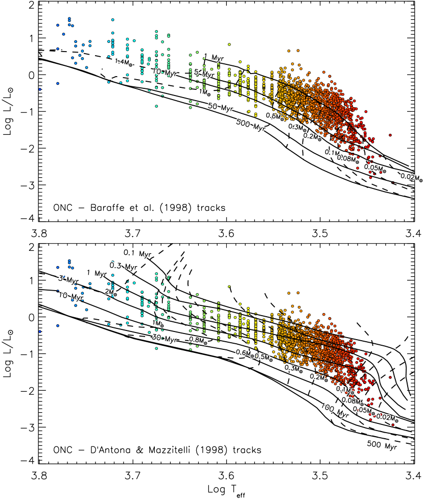
Figure 16.— The H-R diagram of the ONC members, after the removal of contamination from background stars. Evolutionary models are from Baraffe et al. (1998) (upper panel) and D’Antona & Mazzitelli (1998) (lower panel).

Despite the large column density of the Orion molecular cloud, which produces an extinction up to $A_{V}=100$ mag (Bergin et al., 1996; Scandariato et al., 2011), contamination from background stellar populations starts to become non negligible at faint magnitudes in the ONC. In fact, as suggested by previous works, (e.g. Robberto et al., 2010; Hillenbrand & Carpenter, 2000; Muench et al., 2002), the fraction of background contaminants versus members increases towards the substellar mass range in the ONC. This is both due to the increase in the number of faint background sources seen through the Orion molecular cloud, and the decrease of actual members of the young cluster in the BD mass range, because of the declining initial mass function (IMF) at substellar masses (see below).

The contamination from background sources is evident as a large number ($\gtrsim$200 stars) of faint sources in our H-R diagram (Figure 13), which are well separated from the cluster sequence. Given the relatively low $T_{\rm eff}$ for these objects ($\sim 3500$ K$<T_{\rm eff}<\sim 2900$ K), they could be either cool dwarf stars or red giants, the latter more easily detectable at large distances and through the Orion Molecular Cloud. The relative number of these sources, relative to young cluster members, becomes dominant at our detection limit.

A small number of these relatively less-luminous sources might be actual ONC members, whose flux may be masked (e.g., by edge-on circumstellar disks), and therefore are visible only in scattered light. This phenomenon has been observed in several young star-forming regions (see e.g., Guarcello et al., 2010; Kraus & Hillenbrand, 2009, and references therein); however the expected fraction of such objects is very small, including no more than a few percent of the population (De Marchi et al., 2011). On the other hand, the faint sources we detect below the young sequence are about 16% of the total number of stars with $T_{\rm eff}<3200$ K. Therefore, we can assume that most of these sources are actually contaminants. Moreover, removing a small fraction of faint members erroneously considered as background contaminants will not affect significantly the IMF derived in this work, given the small expected number of these objects compared to the entire studied population.

We proceed to attempt to remove the background contamination from the H-R diagram. To this purpose, we define a cut in the H-R diagram such that stars satisfying the following criterion are considered as non-members:

$$\log L<-1.93\ \ \ \log T_{\rm eff}>3.54$$

$$\log L<-5.607$$

$$+65.848 \cdot(\log T_{\rm eff}-3.4)$$

$$-253.02 \cdot(\log T_{\rm eff}-3.4)^{2} \ \ \log T_{\rm eff}<3.54$$

This is shown in Figure 14. All sources located below this line are regarded as non-members and excluded from further analysis. Figure 15 presents the spatial distribution of contaminants in comparison with that of the candidate members. Whereas the latter are centrally concentrated, with an evident north-south elongation, contaminants appear uniformly distributed. Also, we find a slight overabundance of contaminants on the east side of our field of view. The reason for this is that the extinction provided by the Orion Nebula is higher on a central north-south strip, centered on the ONC (Scandariato et al., 2011; Bergin et al., 1996). Therefore the density of background objects is expected to be higher on the two sides of this band. Here, the nebular emission of the OMC is significantly brighter on the west side of our FOV, and this decreases the detection limit in this area. Therefore the east edge of our FOV is expected to show the most prominent density of background contaminants.

In Figure 16 we present once again the H-R diagram of the ONC, now including only our candidate members, together with PMS evolutionary models. In particular, we use isochrones and tracks from either Baraffe et al. (1998) or D’Antona & Mazzitelli (1998). These models, unlike e.g., the Siess et al. (2000) or the Palla & Stahler (1999), also extend into the substellar mass range, and therefore are more suitable for our sample, which reaches masses as low as 0.02 M_⊙ (20M_Jup).

4.3. Completeness in the H-R Diagram

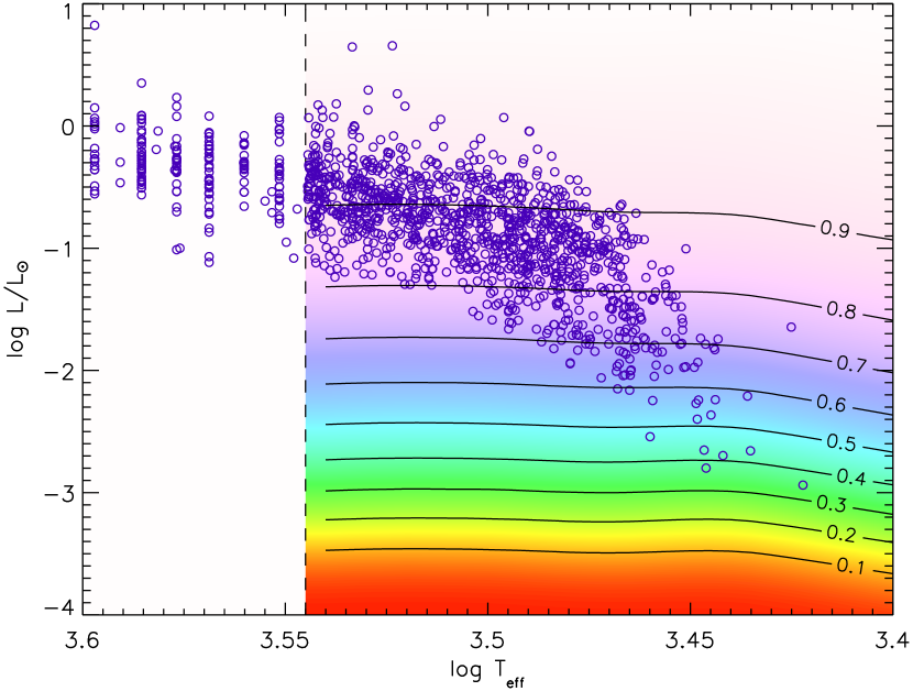
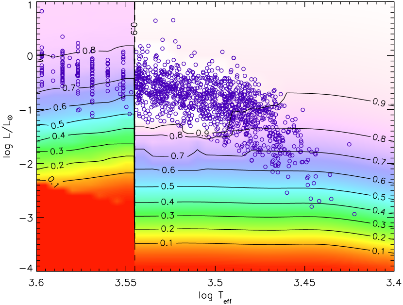
Figure 17.— Completeness function in the H-R diagram, computed accounting for photometric detection and differential reddening as described in the text. The left panel shows the result as computed with our monte-carlo simulation, valid for the spectral types obtained from the medium-band photometry analyzed in this work, for $\log T_{\rm eff}<3.54$ ($T_{\rm eff}<3500$ K). The right panel shows the correction of this completeness after accounting for the additional stars placed in the HRD whose stellar parameters are taken from Paper II.

In Section 2.3 we have derived the photometric completeness of our survey. Starting from this result, we now evaluate the completeness function in the H-R diagram. To do this, we transform the H-R diagram (i.e., $T_{\rm eff}$ and $\log L$) into our observational space (i.e., the 753, 770, and $I$-band magnitudes), and assess the extent to which reddening causes sources of various intrinsic $T_{\rm eff}$ and $\log L$ to be missed in our survey.

We set a uniform, dense grid of $\log T_{\rm eff}$ and $\log L$ bins in the H-R diagram, limited to the region $\log T_{\rm eff}<3.54$. For each bin, we apply in reverse the relations derived in Section 3.1 and 3.4 to derive from $T_{\rm eff}$ and $\log L$ the $[770~{}index]$, the $[A_{V}~{}index]$, and (using the BC) the unreddened $I$-band magnitude, $I_{0}$. Then, by inverting equation 2 and 1, we also derive the magnitudes $m_{753}$ and $m_{770}$. Thus we have associated to each pair of H-R diagram parameters ($\log T_{\rm eff}$,$\log L$) the triplet of intrinsic magnitudes ($m_{753},$$m_{770}$,$I_{0}$) for $A_{V}=0$.

Next we apply reddening to these magnitudes using the empirical reddening distribution of the ONC stellar population. As in Paper II, we limit ourselves to the most luminous half of the ONC population, as these stars sample the full range of $A_{V}$. With a Monte Carlo approach, we draw 1000 $A_{V}$ values from the reddening distribution and apply them to the intrinsic magnitudes ($m_{753},$$m_{770}$,$I_{0}$) associated to each point of the H-R diagram. For every $i$-th ($1<i<1000$) triplet of reddened magnitudes, we compute the photometric completeness $C_{753}(i)$, $C_{770}(i)$, $C_{I}(i)$. The product of these three, $C(i)$, averaged over the 1000 values of $A_{V}$, provides the “differential reddening normalized” completeness for that particular bin in the H-R diagram.

The result is shown in Figure 17a. We find that the completeness is mainly dependent on $\log L$, while its dependence on $T_{\rm eff}$ for a given luminosity is small and appears only at low temperatures ($\log T_{\rm eff}\lesssim 3.45$). We note also that the completeness is rather high ($\sim 50\%$) at the low-mass end of our catalog, and thus even without correcting for the completeness, the observed number of ONC members in the substellar mass range is correct to within a factor of $\sim$2.

Our H-R diagram also includes sources whose stellar parameters are taken from Paper II instead of our new medium-band photometry. For all members with $\log T_{\rm eff}>3.54$, we simply adopt the completeness function in the HRD derived in that paper. In addition, there is a group of stars with $\log T_{\rm eff}<3.54$ but which are not present in our new medium-band photometry and thus whose stellar parameters are from Paper II. The presence of these sources increases the overall completeness in this region of the HRD relative to that computed as above. To account for this, we divide the HRD into a grid with spacing 0.01 dex in $\log T_{\rm eff}$ and 0.1 dex in $\log L$, and we count in each bin the relative number of sources from Paper II versus members classified from our new data. This ratio, smoothed in $\log T_{\rm eff}$ and $\log L$, is added to the completeness shown in Figure 17a.

The final result is shown in Figure 17b. The evident discontinuity in completeness at $\log T_{\rm eff}=3.54$ is due to the fact that for larger $T_{\rm eff}$ the stellar parameters are obtained from optical spectroscopy on an incomplete fraction of sources. From the two-dimensional completeness shown in Figure 17b, we are able to assign a completeness correction to each our sources, allowing us finally to derive a completeness corrected initial mass function for the ONC.

5. The initial mass function

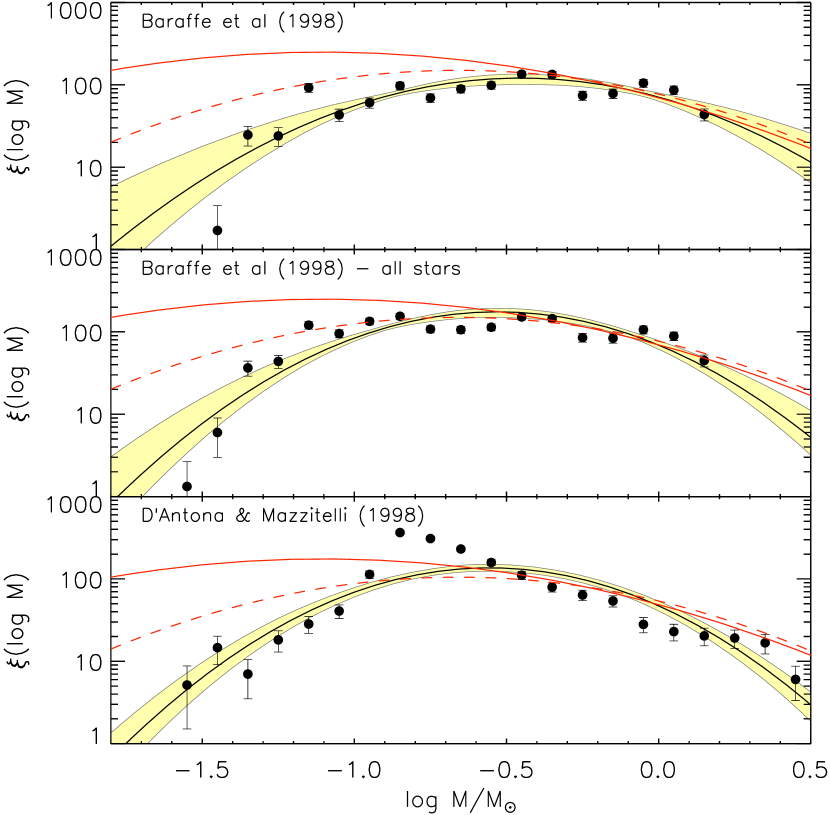
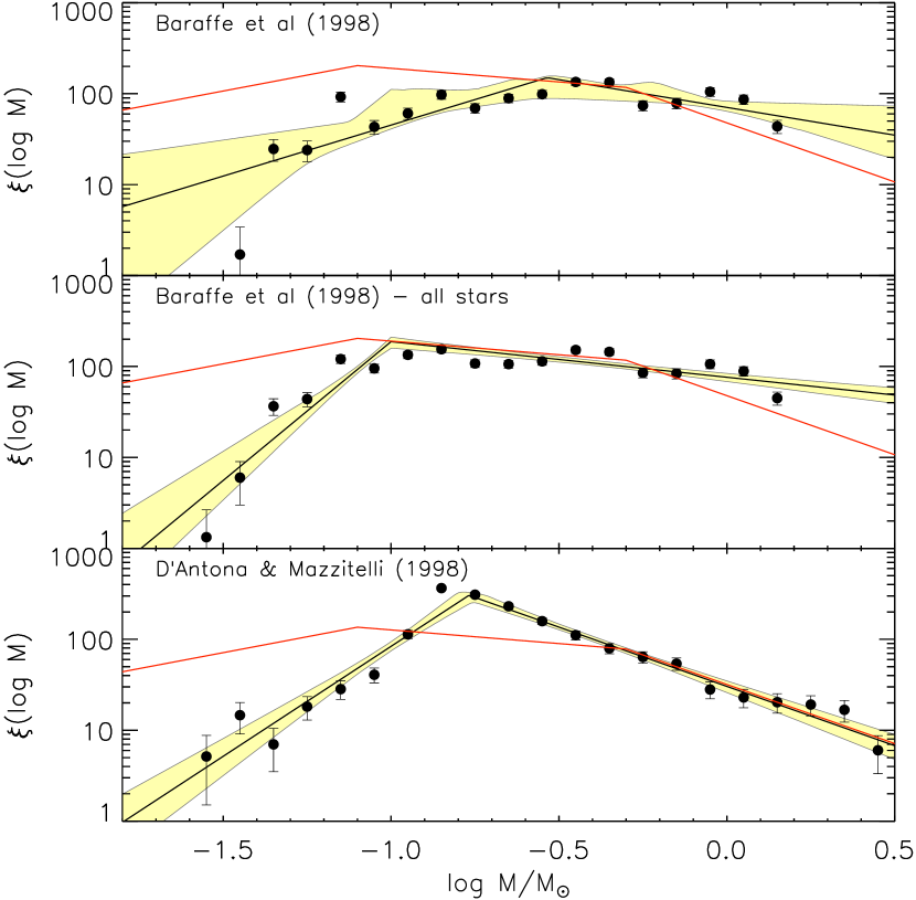
Figure 18.— The measured IMF for the ONC, fitted with a log-normal distribution (left panel) or a two-phase power law (right panel). The top and bottom panels represent the mass distributions obtained assuming Baraffe et al. (1998) and D’Antona & Mazzitelli (1998) models respectively, whereas the center panels show the result assuming Baraffe models and including also stars located above the 1 Myr, whose mass has been extrapolated from their $T_{\rm eff}$ (see text). The shaded areas enclose the 90% confidence interval for each fit. The red curves represent the IMF of Chabrier (2003) (left panel) and Kroupa (2001) (right panel); the red dashed line is the Chabrier (2003) system IMF.

Table 3IMF

	lognormal		2-phase powerlaw
	$\log m_{c}$	$\sigma(\log m)$	$\Gamma_{1}$	$\Gamma_{2}$	$\log m_{c}$
BCAH98	$-0.45\pm 0.02$	$0.44\pm 0.05$	$-1.12\pm 0.90$	$0.60\pm 0.33$	$-0.53\pm 0.26$
BCAH98 all stars	$-0.53\pm 0.02$	$0.39\pm 0.03$	$-3.05\pm 0.53$	$0.39\pm 0.10$	$-1.00\pm 0.08$
DM98	$-0.56\pm 0.02$	$0.38\pm 0.01$	$-2.41\pm 0.25$	$1.30\pm 0.09$	$-0.77\pm 0.02$

Note. — The power law exponents $\Gamma$ follow the standard for which the Salpeter slope is $\Gamma=1.35$

						BCAH98		DM98
ID	R.A.	Dec	$\log T_{\rm eff}$	$\log L_{\rm bol}$	$A_{V}$	M	$\log$ age	M	$\log$ age
	h m s	∘ $\prime$ $\prime\prime$	(K)	($L_{\odot}$)	mag	(M⊙)	(yr)	(M⊙)	(yr)
1	05 34 15.10	-05 23 00.0	3.522 $\pm$ 0.010	-1.553 $\pm$ 0.025	0.000 $\pm$ 0.307	0.243 $\pm$ 0.053	7.305 $\pm$ 0.172	0.255 $\pm$ 0.038	7.308 $\pm$ 0.111
2	05 34 17.26	-05 22 36.7	3.564 $\pm$ 0.010	-1.565 $\pm$ 0.046	0.770 $\pm$ 0.238	0.481 $\pm$ 0.028	8.235 $\pm$ 0.175	0.447 $\pm$ 0.034	8.196 $\pm$ 0.297
3	05 34 17.29	-05 22 48.0	3.492 $\pm$ 0.001	-1.078 $\pm$ 0.018	1.300 $\pm$ 0.096	0.164 $\pm$ 0.006	6.295 $\pm$ 0.020	0.161 $\pm$ 0.002	6.299 $\pm$ 0.017
4	05 34 20.57	-05 21 29.8	3.510 $\pm$ 0.004	-2.312 $\pm$ 0.036	0.971 $\pm$ 0.187	0.168 $\pm$ 0.014	8.090 $\pm$ 0.105	0.185 $\pm$ 0.014	8.260 $\pm$ 0.216
5	05 34 22.40	-05 22 26.9	3.477 $\pm$ 0.002	-1.063 $\pm$ 0.035	0.016 $\pm$ 0.180	$\sim$ 0.098	$<$6	0.136 $\pm$ 0.002	6.239 $\pm$ 0.026
6	05 34 18.37	-05 22 54.9	3.524 $\pm$ 0.010	-2.068 $\pm$ 0.043	0.051 $\pm$ 0.375	0.230 $\pm$ 0.053	8.030 $\pm$ 0.264	0.244 $\pm$ 0.041	8.135 $\pm$ 0.294
7	05 34 20.78	-05 23 29.1	3.530 $\pm$ 0.002	-0.845 $\pm$ 0.027	0.548 $\pm$ 0.115	0.341 $\pm$ 0.012	6.565 $\pm$ 0.036	0.245 $\pm$ 0.006	6.306 $\pm$ 0.035
8	05 34 24.78	-05 22 10.5	3.540 $\pm$ 0.001	-0.643 $\pm$ 0.021	0.266 $\pm$ 0.086	0.429 $\pm$ 0.011	6.470 $\pm$ 0.024	0.275 $\pm$ 0.006	6.142 $\pm$ 0.025
9	05 34 25.64	-05 21 57.6	3.484 $\pm$ 0.001	-1.006 $\pm$ 0.021	0.436 $\pm$ 0.100	0.119 $\pm$ 0.005	6.005 $\pm$ 0.044	0.146 $\pm$ 0.001	6.207 $\pm$ 0.017
10	05 34 26.51	-05 23 23.7	3.497 $\pm$ 0.001	-0.502 $\pm$ 0.013	0.836 $\pm$ 0.055	$\sim$ 0.161	$<$6	0.147 $\pm$ 0.001	5.182 $\pm$ 0.027
…	…	…	…	…	…	…	…	…	…

Table 4(This table is available in its entirety in a machine-readable form in the online journal. A portion is shown here for guidance regarding its form and content.)

To derive the initial mass function (IMF) of the ONC from our observations, we use pre-main-sequence evolutionary models to convert our $T_{\rm eff}$ and $\log L$ from the H-R diagram into masses and ages. We do this using both the D’Antona & Mazzitelli (1998) and Baraffe et al. (1998) models (Figure 16). In the case of Baraffe models, for a large fraction (about 25%) of sources we cannot assign masses and ages, as these stars are located above the 1 Myr isochrone, the minimum age computed for this family of models. This not only decreases our stellar sample, but also biases our findings, in particular the mass distribution. To overcome this selection effect, we consider two cases for the mass estimates from Baraffe models: a) we reject all source above the 1 Myr isochrone; b) we include them by assigning a mass based on the $T_{\rm eff}$-mass relation of the 1 Myr isochrone. Since for very-low mass stars the PMS evolutionary tracks are nearly vertical in the H-R diagram, this approximation is fairly good. In Table 4 we present the derived stellar parameters for the ONC sources, using both sets of models.

From these masses, we derive the mass distribution $\xi(\log m)$ by binning the ONC members in equally-spaced mass bins. For each mass bin, we account for its exact completeness by adding the inverse of the completeness of each source. We associate an uncertainty distribution to each measured value of $\xi(\log m)$ equal to a Possion distribution of mean $\mu=N_{i}$, where $N_{i}$ is the number of sources in the $i-$th bin, scaled by a factor equal to the overall completeness correction for that bin. We stress that, strictly speaking, our mass function is actually a “system” mass function rather than a proper “initial” mass function, in the sense that we do not account for unresolved binaries or multiple systems. This, however, does not influence significantly our results, since the binary fraction (accounting both bound systems and visual binaries) in Orion is small ($\lesssim 15\%$, Padgett et al. 1997; Petr et al. 1998; Reipurth et al. 2007 ), and about half of these are separated more than 1^′′, therefore resolved in our observations.

It it well established (e.g., Bastian et al., 2010) that the IMF generally follows a power-law in the intermediate- and high-mass range ($M\gtrsim M_{\odot}$), whereas for low-mass stars and BDs—which is the region of the mass spectrum most relevant for our study—this function can be approximated with a shallower power law $\xi(\log m)\propto m^{-(\Gamma+1)}$ (e.g., Kroupa, 2001) or with a log-normal distribution $\xi(\log m)\propto e^{-(\log m-\log m_{c})^{2}/2\sigma^{2}}$ (e.g., Chabrier, 2003). We use both forms to fit our measured IMF in the ONC.

We use a Monte Carlo simulation following Da Rio et al. (2009a) to account for the uncertainties in the measured star counts, as follows. For every mass bin, we consider the error bars with their statistical distribution, and generate a large number ($n=10,000$) of points drawn from the error distribution. Then an unweighted fit is run on all these ($n$ times the number of bins) points. The best-fit parameters are isolated using a Levenberg-Marquard minimization algorithm. The uncertainty associated to the parameters has been computed with a sampling technique as follows: for every one of the $m$ bins, we randomly consider only one of the $n$ values previously simulated, i.e. a random sample from the distribution describing the error bar of the bin, and we fit the IMF function on these $m$ data points, deriving the best-fit parameters. By iterating this selection and fit process 1000 times, we derive 1000 sets of parameters. The standard deviation of each parameter for the 1000 tests is the uncertainty in the estimate of the parameter itself.

The resulting fitted functions for both sets of evolutionary models are shown in Figure 18. In Table 3 the fitting parameters are reported: the characteristic mass and the width for the log-normal fit, and the two power law slopes as well as the break point for the 2-phase power law. We find that the two families of evolutionary models lead to significant differences in the derived IMF. Whereas the Baraffe tracks produce a smooth distribution, which appears well fitted by a log-normal distribution characterized by a continuous change in the IMF slope, the D’Antona & Mazzitelli models lead to a more peaked distribution, with an evident maximum at $M\sim 0.15$ M_⊙. The reason for this difference can be attributed to the different shapes of the evolutionary tracks in the very low mass range ($0.3$ M${}_{\odot}\gtrsim M\gtrsim 0.1$ M_⊙), where the models of D’Antona & Mazzitelli predict a larger area of the HRD covered by adjacent tracks. The shape of the IMF derived from the Baraffe et al. models does not depend significantly on which method we adopt for inclusion of very young stars lying above 1 Myr isochrone (see above).

In Figure 18 we also compare our measured mass distribution with standard reference IMFs. In particular we consider the disk IMF from Chabrier (2003) which is expressed as a log-normal function, with a characteristic mass of either 0.079 M_⊙ or 0.22 M_⊙ respectively for the “single objects” IMF or the “system” IMF, the latter not corrected for stellar multiplicity. Also, we consider the universal IMF of Kroupa (2001), which is a multi-phase power law with shallower slopes in the VLMS and BD regime. Depending on the assumed evolutionary models and the type of function fitted, our IMF peaks in the range 0.1 M_⊙ $-$ 0.3 M_⊙, the higher values being larger than that most often reported, even in the case of unresolved multiplicity. This finding, as well as the high dependence on the evolutionary model family used to derive stellar masses, is consistent with what we have found in our previous work (Paper I) limited to the stellar mass range.

A striking feature of our IMF is the steep decline in the BD mass range (see Figure 18); here our mass distribution is much lower than the standard IMFs, implying a significant deficiency of substellar objects in the ONC. We stress that this finding is not biased by detection incompleteness, given that the derived mass distribution has been corrected for completeness star by star, and the completeness function we have derived in Section 4.3 remains fairly high ($\sim 50\%$) even in the BD mass range. Moreover, even hypothesizing an overestimated completeness for the smallest masses in our sample, the relative scarcity of substellar members is evident up to about 0.1 M_⊙; there simply are not many very cool, very low luminosity sources observed. Such a steep decline of the mass function in the BD mass range differs also from IMF determinations in other young regions. In fact the majority of young clusters have been reported to show substellar mass function compatible with the Kroupa or the Chabrier mass distributions. Some examples are Chamaeleon I Luhman (2007), Upper Sco (Lodieu et al., 2007), the $\sigma$ Ori region (Caballero, 2009), $\lambda$ Ori (Bayo et al., 2011), NGC 6611 (Oliveira et al., 2009). Similar findings have also been reported for older open clusters (e.g., Bouvier et al., 2005); in fact for the Praesepe cluster, Wang et al. (2011) measure even an increasing IMF down to $\sim 70$ M_J.

Previous studies of the IMF in the ONC also found a decrease in the relative number of members in the substellar mass range, both in absolute number and relative to the standard IMFs. Studies based on photometry alone (e.g., Hillenbrand & Carpenter, 2000; Muench et al., 2002) using the conversion of near infrared LFs, find a measured IMF slope below the H-burning limit not steeper than $\Gamma\sim-1$, which is the shallowest value we derive assuming Baraffe et al. (1998) models, and up to 2 units flatter than what we derive with D’Antona & Mazzitelli (1998) tracks. Also, Slesnick et al. (2004) finds an IMF for the ONC rapidly decreasing below the H-burning limit, but then flattening in the BD mass range.

Muench et al. (2002) reports a secondary peak in the mass distribution at about the deuterium burning limit ($\sim 0.17$ M_⊙); Slesnick et al. (2004) tentatively find a similar feature, although with less significance and at a slightly higher mass. This mass roughly corresponds to our detection limit. However, from our results, we do not find any evidence of either a flattening of the IMF or an increasing number of sources for the lowest mass bins. We interpret this inconsistency as an inaccurate estimate of the background contamination in previous works, which we believe is much improved through the methodology that we have developed here.

Based on our measured IMF, complemented in the intermediate- and high mass range using the results from Hillenbrand (1997), we assess a total stellar mass for the ONC of about $10^{3}$ M_⊙.

References

- Allard et al. (2010) Allard, F., Homeier, D., & Freytag, B. 2010, ASP Conf. Ser., Cool Star 16, in press (arXiv:1011.5405)
- Allard et al. (2000) Allard, F., Hauschildt, P. H., & Schwenke, D. 2000, ApJ, 540, 1005
- Baraffe et al. (1998) Baraffe, I., Chabrier, G., Allard, F., et al. 1998, A&A, 337, 403
- Bastian et al. (2010) Bastian, N., Covey, K. R., & Meyer, M. R. 2010, ARA&A, 48, 339
- Bayo et al. (2011) Bayo, A., Barrado, D., Stauffer, J., et al. 2011, arXiv:1109.4917
- Bergin et al. (1996) Bergin, E. A., Snell, R. L., & Goldsmith, P. F. 1996, ApJ, 460, 343
- Bessell et al. (1998) Bessell, M. S., Castelli, F., & Plez, B. 1998, A&A, 333, 231
- Bouvier et al. (2005) Bouvier, J., Moraux, E., & Stauffer, J. 2005, The Initial Mass Function 50 Years Later, 327, 61
- Caballero (2009) Caballero, J. A. 2009, American Institute of Physics Conference Series, 1094, 912
- Calvet & Gullbring (1998) Calvet, N., & Gullbring, E. 1998, ApJ, 509, 802
- Cardelli et al. (1989) Cardelli, J. A., Clayton, G. C., & Mathis, J. S. 1989, ApJ, 345, 245
- Chabrier (2003) Chabrier, G. 2003, PASP, 115, 763
- Cohen & Kuhi (1979) Cohen, M., & Kuhi, L. V. 1979, ApJS, 41, 743
- Costero & Peimbert (1970) Costero, R., & Peimbert, M. 1970, Boletin de los Observatorios Tonantzintla y Tacubaya, 5, 229
- D’Antona & Mazzitelli (1998) D’Antona, F., & Mazzitelli, I. 1998, Brown Dwarfs and Extrasolar Planets, 134, 442
- Da Rio et al. (2010) Da Rio, N., Robberto, M., Soderblom, D. R., et al. 2010, ApJ, 722, 1092
- Da Rio et al. (2009b) Da Rio, N., Robberto, M., Soderblom, D. R., et al. 2009, ApJS, 183, 261
- Da Rio et al. (2009a) Da Rio, N., Gouliermis, D. A., & Henning, T. 2009, ApJ, 696, 528
- De Marchi et al. (2011) De Marchi, G., Panagia, N., Guarcello, et al. 2010, A&Asubmitted
- Fischer et al. (2011) Fischer, W., Edwards, S., Hillenbrand, L., et al. 2011, ApJ, 730, 73
- Flower (1996) Flower, P. J. 1996, ApJ, 469, 355
- Guarcello et al. (2010) Guarcello, M. G., Damiani, F., Micela, G., et al. 2010, A&A, 521, A18
- Hillenbrand (1997) Hillenbrand, L. A. 1997, AJ, 113, 1733
- Hillenbrand & Carpenter (2000) Hillenbrand, L. A., & Carpenter, J. M. 2000, ApJ, 540, 236
- Kraus & Hillenbrand (2009) Kraus, A. L., & Hillenbrand, L. A. 2009, ApJ, 703, 1511
- Kroupa (2002) Kroupa, P. 2002, Science, 295, 82
- Kroupa (2001) Kroupa, P. 2001, MNRAS, 322, 231
- Lodieu et al. (2007) Lodieu, N., Hambly, N. C., Jameson, R. F., et al. 2007, MNRAS, 374, 372
- Lucas et al. (2006) Lucas, P. W., Weights, D. J., Roche, P. F., et al. 2006, MNRAS, 373, L60
- Lucas et al. (2005) Lucas, P. W., Roche, P. F., & Tamura, M. 2005, MNRAS, 361, 211
- Lucas et al. (2001) Lucas, P. W., Roche, P. F., Allard, F., et al. 2001, MNRAS, 326, 695
- Lucas & Roche (2000) Lucas, P. W., & Roche, P. F. 2000, MNRAS, 314, 858
- Luhman et al. (2000) Luhman, K. L., Rieke, G. H., Young, E. T., et al. 2000, ApJ, 540, 1016
- Luhman (2007) Luhman, K. L. 2007, ApJS, 173, 104
- Menten et al. (2007) Menten, K. M., Reid, M. J., Forbrich, J., et al. 2007, A&A, 474, 515
- Meyer et al. (1997) Meyer, M. R., Calvet, N., & Hillenbrand, L. A. 1997, AJ, 114, 288
- Muench et al. (2002) Muench, A. A., Lada, E. A., Lada, C. J., et al. 2002, ApJ, 573, 366
- Muench et al. (2000) Muench, A. A., Lada, E. A., & Lada, C. J. 2000, ApJ, 533, 358
- Oliveira et al. (2009) Oliveira, J. M., Jeffries, R. D., & van Loon, J. T. 2009, MNRAS, 392, 1034
- Padgett et al. (1997) Padgett, D. L., Strom, S. E., & Ghez, A. 1997, ApJ, 477, 705
- Palla & Stahler (1999) Palla, F., & Stahler, S. W. 1999, ApJ, 525, 772
- Petr et al. (1998) Petr, M. G., Coudé du Foresto, V., Beckwith, S. V. W., et al. 1998, ApJ, 500, 825
- Reipurth et al. (2007) Reipurth, B., Guimarães, M. M., Connelley, M. S., et al. 2007, AJ, 134, 2272
- Reggiani et al. (2011) Reggiani, M., Robberto, M., Da Rio, N., et al. 2011, A&A, 534, A83
- Riddick et al. (2007) Riddick, F. C., Roche, P. F., & Lucas, P. W. 2007, MNRAS, 381, 1077
- Robberto et al. (2010) Robberto, M., Soderblom, D. R., Scandariato G., et al. 2010, AJ, 139, 950
- Robberto et al. (2005) Robberto, M., et al. 2005, Bulletin of the American Astronomical Society, 37, #146.01
- Salpeter (1955) Salpeter, E. E. 1955, ApJ, 121, 161
- Scandariato et al. (2011) Scandariato, G., Robberto, M., Pagano, I., et al. 2011, A&A, 533, A38
- Siess et al. (2000) Siess, L., Dufour, E., Forestini, M. 2000, A&A, 358, 593
- Slesnick et al. (2004) Slesnick, C. L., Hillenbrand, L. A., & Carpenter, J. M. 2004, ApJ, 610, 1045
- Stetson (1987) Stetson, P. B. 1987, PASP, 99, 191
- Vandame (2004) Vandame, B., PhD thesis, Nice University, 2004
- Wang et al. (2011) Wang, W., Boudreault, S., Goldman, B., et al. 2011, A&A, 531, A164
- Weights et al. (2009) Weights, D. J., Lucas, P. W., Roche, P. F., et al. 2009, MNRAS, 392, 817