Truncated Power Method for Sparse Eigenvalue Problems

Abstract

This paper considers the sparse eigenvalue problem, which is to extract dominant (largest) sparse eigenvectors with at most $k$ non-zero components. We propose a simple yet effective solution called truncated power method that can approximately solve the underlying nonconvex optimization problem. A strong sparse recovery result is proved for the truncated power method, and this theory is our key motivation for developing the new algorithm. The proposed method is tested on applications such as sparse principal component analysis and the densest $k$-subgraph problem. Extensive experiments on several synthetic and real-world large scale datasets demonstrate the competitive empirical performance of our method.

1 Introduction

Given a $p\times p$ symmetric positive semidefinite matrix $A$, the largest $k$-sparse eigenvalue problem aims to maximize the quadratic form $x^{\top}Ax$ with a sparse unit vector $x\in\mathbb{R}^{p}$ with no more than $k$ non-zero elements:

$$\lambda_{\max}(A,k)=\max_{x\in\mathbb{R}^{p}}x^{\top}Ax,\ \ \ \ \ \ \ \text{subject to }\|x\|=1,\|x\|_{0}\leq k,$$ (1.1)

where $\|\cdot\|$ denotes the $\ell_{2}$-norm, and $\|\cdot\|_{0}$ denotes the $\ell_{0}$-norm which counts the number of non-zero entries in a vector. The sparsity is controlled by the values of $k$ and can be viewed as a design parameter. In machine learning applications, e.g., principal component analysis, this problem is motivated from the following perturbation formulation of matrix $A$:

$$A=\bar{A}+E,$$ (1.2)

where $A$ is the empirical covariance matrix, $\bar{A}$ is the true covariance matrix, and $E$ is a random perturbation due to having only a finite number of empirical samples. If we assume that the largest eigenvector $\bar{x}$ of $\bar{A}$ is sparse, then a natural question is to recover $\bar{x}$ from the noisy observation $A$ when the error $E$ is “small”. In this context, the problem (1.1) is also referred to as sparse principal component analysis (sparse PCA).

In general, problem (1.1) is non-convex. In fact, it is also NP-hard because it can be reduced to the subset selection problem for ordinary least squares regression (Moghaddam et al., 2006), which is known to be NP hard. Various researchers have proposed approximate optimization methods: some are based on greedy procedures (e.g., Moghaddam et al., 2006; Jolliffe et al., 2003; d’Aspremont et al., 2008), and some others are based on various types of convex relaxation or reformulation (e.g., d’Aspremont et al., 2007; Zou et al., 2006; Journée et al., 2010). Although many algorithms have been proposed, almost no satisfactory theoretical results exist for this problem. The only exception is the analysis of the convex relaxation method (d’Aspremont et al., 2007) by Amini & Wainwright (2009) under the high dimensional spiked covariance model (Johnstone, 2001). However, the result was concerned with variable selection consistency under a very simple and specific example with limited general applicability.

This paper proposes a new computational procedure called truncated power iteration method that approximately solves (1.1). This method is similar to the classical power method, with an additional truncation operation to ensure sparsity. We show that if the true matrix $\bar{A}$ has a sparse (or approximately sparse) dominant eigenvector $\bar{x}$, then under appropriate assumptions, this algorithm can recover $\bar{x}$ when the spectral norm of sparse submatrices of the perturbation $E$ is small. Moreover, this result can be proved under relative generality without restricting ourselves to the rather specific spiked covariance model. Therefore our analysis provides strong theoretical support for this new method, and this differentiates our proposal from previous studies. We have applied the proposed method to sparse PCA and to the densest $k$-subgraph finding problem (with proper modification). Extensive experiments on synthetic and real-world large scale datasets demonstrate both the competitive sparse recovering performance and the computational efficiency of our method.

It is worth mentioning that the truncated power method developed in this paper can also be applied to the smallest $k$-sparse eigenvalue problem given by:

$$\lambda_{\min}(A,k)=\min_{x\in\mathbb{R}^{p}}\;x^{\top}Ax,\ \ \ \ \ \ \ \text{subject to }\|x\|=1,\quad\|x\|_{0}\leq k,$$

which also has many applications in machine learning.

1.1 Notation

Let $\mathbb{S}^{p}=\{A\in\mathbb{R}^{p\times p}\mid A=A^{\top}\}$ denote the set of symmetric matrices, and $\mathbb{S}_{+}^{p}=\{A\in\mathbb{S}^{p},A\succeq 0\}$ denote the cone of symmetric, positive semidefinite (PSD) matrices. For any $A\in\mathbb{S}^{p}$, we denote its eigenvalues by $\lambda_{\min}(A)=\lambda_{p}(A)\leq\cdots\leq\lambda_{1}(A)=\lambda_{\max}(A)$. We use $\rho(A)$ to denote the spectral norm of $A$, which is $\max\{|\lambda_{\min}(A)|,|\lambda_{\max}(A)|\}$, and define $\rho(A,s):=\max\{|\lambda_{\min}(A,s)|,|\lambda_{\max}(A,s)|\}$. The $i$-th entry of vector $x$ is denoted by $[x]_{i}$ while $[A]_{ij}$ denotes the element on the $i$-th row and $j$-th column of matrix $A$. We denote by $A_{k}$ any $k\times k$ principal submatrix of $A$ and by $A_{F}$ the principal submatrix of $A$ with rows and columns indexed in set $F$. If necessary, we also denote $A_{F}$ as the restriction of $A$ on the rows and columns indexed in $F$. Let $\|x\|_{p}$ be the $\ell_{p}$-norm of a vector $x$. In particular, $\|x\|_{2}=\sqrt{x^{\top}x}$ denotes the Euclidean norm, $\|x\|_{1}=\sum_{i=1}^{d}|[x]_{i}|$ denotes the $\ell_{1}$-norm, and $\|x\|_{0}=\#\{j:[x]_{j}\neq 0\}$ denotes the $\ell_{0}$-norm. For simplicity, we also denote the $\ell_{2}$ norm $\|x\|_{2}$ by $\|x\|$. In the rest of the paper, we define $Q(x):=x^{\top}Ax$ and let $x_{*}$ be the optimal solution of problem (1.1). We let $\text{supp}(x):=\{j:\mid[x]_{j}\neq 0\}$ denote the support set of the vector $x$. Given an index set $F$, we define

$$x(F):=\mathop{\arg\max}_{x\in\mathbb{R}^{p}}x^{\top}Ax,\ \ \ \text{subject to }\|x\|=1,\quad\text{supp}(x)\subseteq F.$$

Finally, we denote by $I_{p\times p}$ the $p\times p$ identity matrix.

1.2 Paper Organization

The remaining of this paper is organized as follows: Section 2 describes the truncated power iteration algorithm that approximately solves problem (1.1). In Section 3 we analyze the solution quality of the proposed algorithm. Section 4 evaluates the practical performance of the proposed algorithm in applications of sparse PCA and the densest $k$-subgraph finding problems. We conclude this work and discuss potential extensions in Section 5.

2 Truncated Power Method

Since $\lambda_{\max}(A,k)$ equals $\lambda_{\max}(A^{*}_{k})$ where $A^{*}_{k}$ is the $k\times k$ principal submatrix of $A$ with the largest eigenvalue, one may solve (1.1) by exhaustively enumerate all subsets of $\{1,\ldots,p\}$ of size $k$ in order to find $A^{*}_{k}$. However, this procedure is impractical even for moderate sized $k$ since the number of subsets is exponential in $k$.

Therefore in order to solve the spare eigenvalue problem (1.1) more efficiently, we consider an iterative procedure based on the standard power method for eigenvalue problems, while maintaining the desired sparsity for the intermediate solutions. The procedure, presented in Algorithm 2, generates a sequence of intermediate $k$-sparse eigenvectors $x_{0},x_{1},\ldots$ from an initial sparse approximation $x_{0}$. At each step $t$, the intermediate vector $x_{t-1}$ is multiplied by $A$, and then the entries are truncated to zeros except for the largest $k$ entries. The resulting vector is then normalized to unit length, which becomes $x_{t}$. It will be assumed throughout the paper that the cardinality $k$ of $\text{supp}(x_{*})$ is available a prior; in practice this quantity may be regarded as a tuning parameter of the algorithm.

Definition 1.

Given a vector $x$ and an index set $F$, we define the truncation operation $\text{Truncate}(x,F)$ to be the vector obtained by restricting $x$ to $F$, that is

$$[\text{Truncate}(x,F)]_{i}=\left\{\begin{array}[]{l}[x]_{i}\ \ \ i\in F\\ 0\ \ \ \ \ \ \text{otherwise}\end{array}\right..$$

Input : matrix $A\in\mathbb{S}^{p}$, initial vector $x_{0}\in\mathbb{R}^{p}$

Output : $x_{t}$

Parameters : cardinality $k\in\{1,...,p\}$

Let $t=1$.

repeat

      

      Compute $x^{\prime}_{t}=Ax_{t-1}/\|Ax_{t-1}\|$.

      Let $F_{t}=\text{supp}(x^{\prime}_{t},k)$ be the indices of $x^{\prime}_{t}$ with the largest $k$ absolute values.

      Compute $\hat{x}_{t}=\text{Truncate}(x^{\prime}_{t},F_{t})$.

      Normalize $x_{t}=\hat{x}_{t}/\|\hat{x}_{t}\|$.

      $t\leftarrow t+1$.

until Convergence;

Algorithm 1 Truncated Power (TPower) Method

Remark 1.

Similar to the behavior of traditional power method, if $A\in\mathbb{S}_{+}^{p}$, then TPower tries to find the (sparse) eigenvector of $A$ corresponding to the largest eigenvalue. Otherwise, it may find the (sparse) eigenvector with the smallest eigenvalue if $-\lambda_{p}(A)>\lambda_{1}(A)$. However, this situation is easily detectable because it can only happen when $\lambda_{p}(A)<0$. In such case, we may restart TPower with $A$ replaced by an appropriately shifted version $A+\tilde{\lambda}I_{p\times p}$.

3 Sparse Recovery Analysis

We consider the general noisy matrix model (1.2), and are specially interested in the high dimensional situation where the dimension $p$ of $A$ is large. We assume that the noise matrix $E$ is a dense $p\times p$ matrix such that its sparse submatrices have small spectral norm $\rho(E,s)$ for $s$ in the same order of $k$. We refer to this quantity as restricted perturbation error. However, the spectral norm of the full matrix perturbation error $\rho(E)$ can be large. For example, if the original covariance is corrupted by an additive standard Gaussian iid noise vector, then $\rho(E,s)=O(\sqrt{s\log p/n})$, which grows linearly in $\sqrt{s}$, instead of $\rho(E)=O(\sqrt{p/n})$, which grows linearly in $\sqrt{p}$. The main advantage of the sparse eigenvalue formulation (1.1) over the standard eigenvalue formulation is that the estimation error of its optimal solution depends on $\rho(E,s)$ with respectively a small $s=O(k)$ rather than $\rho(E)$. This linear dependency on sparsity $k$ instead of the original dimension $p$ is analogous to similar results for sparse regression (or compressive sensing) such as (Candes & Tao, 2005). In fact the restricted perturbation error considered here is analogous to the idea of restricted isometry property (RIP) considered in (Candes & Tao, 2005).

The purpose of the section is to show that if matrix $\bar{A}$ has a unique sparse (or approximately sparse) dominant eigenvector, then under suitable conditions, TPower can (approximately) recover this eigenvector from the noisy observation $A$.

Assumption 1.

Assume that the largest eigenvalue of $\bar{A}\in\mathbb{S}^{p}$ is $\lambda=\lambda_{\max}(\bar{A})>0$ that is non-degenerate, with a gap $\Delta\lambda=\lambda-\max_{j>1}|\lambda_{j}(\bar{A})|$ between the largest and the remaining eigenvalues. Moreover, assume that the eigenvector $\bar{x}$ corresponding to the dominant eigenvalue $\lambda$ is sparse with cardinality $\bar{k}=\|\bar{x}\|_{0}$.

We want to show that under Assumption 1, if the spectral norm $\rho(E,s)$ of the error matrix is small for an appropriately chosen $s>\bar{k}$, then it is possible to approximately recover $\bar{x}$. Note that in the extreme case of $s=p$, this result follows directly from the standard eigenperturbation analysis (which does not require Assumption 1).

We now state our main result as below, which shows that under appropriate conditions, the TPower method can recover the sparse eigenvector. The final error bound is a direct generalization of standard matrix perturbation result that depends on the full matrix perturbation error $\rho(E)$. Here this quantity is replaced by the restricted perturbation error $\rho(E,s)$.

Theorem 1.

We assume that Assumption 1 holds. Let $s=2k+\bar{k}$ with $k\geq 4\bar{k}$. Assume that $\rho(E,s)\leq\Delta\lambda/2$. Define

$$\gamma(s):=\frac{\lambda-\Delta\lambda+\rho(E,s)}{\lambda-\rho(E,s)}<1,\qquad\delta(s):=\frac{\sqrt{2}\rho(E,s)}{\sqrt{\rho(E,s)^{2}+(\Delta\lambda-2\rho(E,s))^{2}}}.$$

If $|x_{0}^{\top}\bar{x}|\geq u+\delta(s)$ for some $\|x_{0}\|_{0}\leq k$, $\|x_{0}\|=1$, and $u\in[0,1]$ such that

$$\mu_{1}= (1-\gamma(s)^{2})u(1-u^{2})/2-\left(2\delta(s)+(\bar{k}/k)^{1/2}\right)\in(0,1),$$

$$\mu_{2}= \sqrt{(1+3(\bar{k}/k)^{1/2})(1-0.45(1-\gamma(s)^{2}))}<1,$$

then let $\mu=\max(\sqrt{1-\mu_{1}},\mu_{2})$, we have

$$\sqrt{1-|x_{t}^{\top}\bar{x}|}\leq\mu^{t}\sqrt{1-|x_{0}^{\top}\bar{x}|}+\sqrt{5}\delta(s)/(1-\mu_{2}).$$

Remark 2.

We only state our result with a relatively simple but easy to understand quantity $\rho(E,s)$, which we refer to as restricted perturbation error. It is analogous to the RIP concept in (Candes & Tao, 2005), and is also directly comparable to the traditional full matrix perturbation error $\rho(E)$. While it is possible to obtain sharper results with additional quantities, we intentionally keep the theorem simple so that its consequence is relatively easy to interpret.

Remark 3.

Although we state the result by assuming that the dominant eigenvector $\bar{x}$ is sparse, the theorem can also be applied to certain situations that $\bar{x}$ is only approximately sparse. In such case, we simply let $\bar{x}^{\prime}$ be a $\bar{k}$ sparse approximation of $\bar{x}$. If $\bar{x}^{\prime}-\bar{x}$ is sufficiently small, then $\bar{x}^{\prime}$ is the dominant eigenvector of a symmetric matrix $\bar{A}^{\prime}$ that is close to $\bar{A}$; hence the theorem can be applied with the decomposition $A=\bar{A}^{\prime}+E^{\prime}$ where $E^{\prime}=E+A-\bar{A}^{\prime}$.

Note that we did not make any attempt to optimize the constants in Theorem 1, which are relatively large. Therefore in the discussion, we shall ignore the constants, and focus on the main message of Theorem 1. If $\rho(E,s)$ is smaller than the eigen-gap $\Delta\lambda/2>0$, then $\gamma(s)<1$ and $\delta(s)=O(\rho(E,s))$. It follows that under appropriate conditions, as long as we can find an initial $x_{0}$ such that

$$|x_{0}^{\top}\bar{x}|\geq c(\rho(E,s)+(\bar{k}/k)^{1/2})$$

for some constant $c$, then $1-|x_{t}^{\top}\bar{x}|$ converges geometrically until

$$\|x_{t}-\bar{x}\|^{2}=O(\rho(E,s)^{2}).$$

This result is similar to the standard eigenvector perturbation result stated in Lemma 2 of Appendix A, except that we replace the spectral error $\rho(E,p)$ of the full matrix by $\rho(E,s)$ that can be significantly smaller when $s\ll p$. To our knowledge, this is the first sparse recovery result for the sparse eigenvalue problem in a relatively general setting. This theorem can be considered as a strong theoretical justification of the proposed TPower algorithm that distinguishes it from earlier algorithms without theoretical guarantees. Specifically, the replacement of the full matrix perturbation error $\rho(E)^{2}$ with $\rho(E,s)^{2}$ gives the theoretical insights on why TPower works well in practice.

To illustrate our result, we briefly describe a consequence of the theorem under the spiked covariance model of (Johnstone, 2001) which was investigated by Amini & Wainwright (2009). We assume that the observations are $p$ dimensional vectors

$$x_{i}=\bar{x}+\epsilon,$$

for $i=1,\ldots,n$, where $\epsilon\sim N(0,I_{p\times p})$. For simplicity, we assume that $\|\bar{x}\|=1$. The true covariance is

$$\bar{A}=\bar{x}\bar{x}^{\top}+I_{p\times p},$$

and $A$ is the empirical covariance

$$A=\frac{1}{n}\sum_{i=1}^{n}x_{i}x_{i}^{\top}.$$

Let $E=A-\bar{A}$, then random matrix theory implies that with large probability,

$$\rho(E,s)=O(\sqrt{s\ln p/n}).$$

Now assume that $\max_{j}|\bar{x}_{j}|$ is sufficiently large. In this case, we can run TPower with a starting point $x_{0}=e_{j}$ for some vector $e_{j}$ (where $e_{j}$ is the vector of zeros except the $j$-th entry being one) so that $|e_{j}^{\top}\bar{x}|=|\bar{x}_{j}|$ is sufficiently large, and the assumption for the initial vector $|x_{0}^{\top}\bar{x}|\geq c(\rho(E,s)+(\bar{k}/k)^{1/2})$ is satisfied with $s=O(\bar{k})$. We may run TPower with an appropriate initial vector to obtain an approximate solution $x_{t}$ of error

$$\|x_{t}-\bar{x}\|^{2}=O(\bar{k}\ln p/n).$$

This is optimal. Note that our results are not directly comparable to those of Amini & Wainwright (2009), which studied support recovery. Nevertheless, it is worth noting that if $\max_{j}|\bar{x}_{j}|$ is sufficiently large, then our result becomes meaningful when $n=O(\bar{k}\ln p)$; however their result requires $n=O(\bar{k}^{2}\ln p)$ to be meaningful, although this is for the pessimistic case of $\bar{x}$ having equal nonzero values of $1/\sqrt{\bar{k}}$.

Finally we note that if we cannot find a large initial value with $|x_{0}^{\top}\bar{x}|$, then it may be necessary to take a relatively large $k$ so that the requirement $|x_{0}^{\top}\bar{x}|\geq c((\bar{k}/k)^{1/2})$ is satisfied. With such a $k$, $\rho(E,s)$ may be relatively large and hence the theorem indicates that $x_{t}$ may not converge to $\bar{x}$ accurately. Nevertheless, as long as $|x_{t}^{\top}\bar{x}|$ converges to a value that is not too small (e.g., can be much larger than $|x_{0}^{\top}\bar{x}|$), we may reduce $k$ and rerun the algorithm with $x_{t}$ as initial vector together with a small $k$. In this two stage process, the vector found from the first stage (with large $k$) is used to as the initial value of the second stage (with small $k$). Therefore we may also regard it as an initialization method to TPower. In practice, one may use other methods to obtain an approximate $x_{0}$ to initialize TPower, not necessarily restricted to running TPower with larger $k$. Some practical alternatives are discussed in Section 4.

4 Applications

In this section, we illustrate the effectiveness of TPower method when applied to sparse principal component analysis (sparse PCA) (in Section 4.1) and the densest $k$-subgraph (DkS) finding problem (in Section 4.2). The Matlab code for reproducing the experimental results reported in this section is online available at https://sites.google.com/site/xtyuan1980/publications.

4.1 Sparse PCA

Principal component analysis (PCA) is a well established tool for dimensionality reduction and has a wide range of applications in science and engineering where high dimensional datasets are encountered. Sparse principal component analysis (sparse PCA) is an extension of PCA that aims at finding sparse vectors (loading vectors) capturing the maximum amount of variance in the data. In recent years, various researchers have proposed various approaches to directly address the conflicting goals of explaining variance and achieving sparsity in sparse PCA. For instance, Zou et al. (2006) formulated sparse PCA as a regression-type optimization problem and imposed the Lasso (Tibshirani, 1996) penalty on the regression coefficients. The DSPCA algorithm in (d’Aspremont et al., 2007) is an $\ell_{1}$-norm based semidefinite relaxation for sparse PCA. Shen & Huang (2008) resorted to the singular value decomposition (SVD) to compute low-rank matrix approximations of the data matrix under various sparsity-inducing penalties. Greedy search and branch-and-bound methods were investigated in (Moghaddam et al., 2006) to solve small instances of sparse PCA exactly and to obtain approximate solutions for larger scale problems. More recently, d’Aspremont et al. (2008) proposed the use of greedy forward selection with a certificate of optimality, and Journée et al. (2010) studied a generalized power method to solve sparse PCA with a certain dual reformulation of the problem. In comparison, our method works directly in the primal domain, and the resulting algorithm is quite different from that of Journée et al. (2010).

Given a sample covariance matrix, $\Sigma\in\mathbb{S}_{+}^{p}$ (or equivalently a centered data matrix $D\in\mathbb{R}^{n\times p}$ with $n$ rows of $p$-dimensional observations vectors such that $\Sigma=D^{\top}D$) and the target cardinality $k$, following  (Moghaddam et al., 2006; d’Aspremont et al., 2007, 2008), we formulate sparse PCA as:

$$\hat{x}=\mathop{\arg\max}_{x\in\mathbb{R}^{p}}x^{\top}\Sigma x,\ \ \ \ \ \ \ \text{subject to }\|x\|=1,\|x\|_{0}\leq k.$$ (4.1)

The TPower method proposed in this paper can be directly applied to solve the above problem. One advantage of TPower for Sparse PCA is that it directly addresses the constraint on cardinality $k$. To find the top $m$ rather than the top one sparse loading vectors, a common approach in the literature (d’Aspremont et al., 2007; Moghaddam et al., 2006; Mackey, 2008) is to use the iterative deflation method for PCA: subsequent sparse loading vectors can be obtained by recursively removing the contribution of the previously found loading vectors from the covariance matrix. Here we employ a projection deflation scheme from (Mackey, 2008), which deflates an vector $\hat{x}$ using the formula:

$$\Sigma^{\prime}=(I_{p\times p}-\hat{x}\hat{x}^{\top})\Sigma(I_{p\times p}-\hat{x}\hat{x}^{\top}).$$

Obviously, $\Sigma^{\prime}$ remains positive semidefinite. Moreover, $\Sigma^{\prime}$ is rendered left and right orthogonal to $\hat{x}$.

4.1.1 Connection with Existing Sparse PCA Methods

In the setup of sparse PCA, TPower is closely related to GPower (Journée et al., 2010) and sPCA-rSVD (Shen & Huang, 2008) which are both power-truncation-type iterative algorithms. Indeed, GPower and sPCA-rSVD are identical except for the initialization and post-processing phases (Journée et al., 2010). Given a data matrix $D\in\mathbb{R}^{n\times p}$, the $\ell_{1}$-norm version of GPower (and equivalently sPCA-rSVD) solves the following regularized rank-1 approximation problem:

$$\min_{x\in\mathbb{R}^{p},z\in\in\mathbb{R}^{n}}\|D-zx^{\top}\|_{F}^{2}+\gamma\|x\|_{1},\ \ \ \text{subject to }\|z\|=1,$$

while the $\ell_{0}$-norm version of GPower (and sPCA-rSVD) solves the following optimization problem:

$$\min_{x\in\mathbb{R}^{p},z\in\in\mathbb{R}^{n}}\|D-zx^{\top}\|_{F}^{2}+\gamma\|x\|_{0},\ \ \ \text{subject to }\|z\|=1.$$

Given the covariance matrix $\Sigma=D^{\top}D$, it is easy to verify that TPower optimizes the following constrained low-1 and semidefinite approximation problem

$$\min_{x\in\mathbb{R}^{p}}\|\Sigma-xx^{\top}\|_{F}^{2},\ \ \ \text{subject to }\|x\|=1,\ \|x\|_{0}\leq k.$$

Essentially, TPower, GPower and sPCA-rSVD all use certain power-truncation type procedure to generate sparse loadings. However, the difference between TPower and GPower (sPCA-rSVD) is also clear: the former performs rank-1, semidefinite and sparse approximation to covariance matrix while the latter performs rank-1 and sparse approximation to the data matrix. One important benefit of TPower is that we are able to analyze solution quality such as sparse recovery capability, while analogous results are not available for GPower and sPCA-rSVD.

Our method is also related to PathSPCA (d’Aspremont et al., 2008) that directly addresses the formulation (1.1). The PathSPCA method is a greedy forward selection procedure which starts from the empty set and at each iteration it selects the most relevant variable and adds it to the current variable set; it then re-estimates the leading eigenvector on the augmented variable set. Both TPower and PathSPCA output sparse solutions with exact cardinality $k$.

4.1.2 On Initialization

Theorem 1 suggests that the TPower algorithm can benefit from a good initial vector $x_{0}$. In a practical implementation, the following three initialization schemes can be considered.

• One simple method is to set $[x_{0}]_{j}=1$ on index $j=\mathop{\arg\max}_{i}[A]_{ii}$ and $0$ otherwise. This initialization provides a $1/k$-approximation to the optimal value, i.e., $Q(x_{0})\geq\lambda_{\max}(A,k)/k$. Indeed, if we let $A^{*}_{k}$ be the $k\times k$ principle submatrix of $A$ supported on $\text{supp}(x_{*})$, then it is easy to verify that $[A]_{jj}\geq\text{Tr}(A^{*}_{k})/k\geq\lambda_{\max}(A,k)/k$. In the setup of sparse PCA, this corresponds to initializing by selecting the variable with the largest variance, which is known to perform well for PathSPCA (d’Aspremont et al., 2008). Alternatively, we may initialize $x_{0}$ as the indicator vector of the top $k$ values of the variances $\{[A]_{ii}\}$, as is considered by Amini & Wainwright (2009).

• A two-stage warm-start strategy suggested at the end of Section 3. In the first stage we may run TPower with a relatively large $k$ and use the output as the initial value of the next stage with a decreased $k$. Repeat this procedure if necessary until the desired cardinality is reached. More generally, one may use other algorithms to warm start TPower.

• When $k\approx p$, an initialization scheme suggested in (Moghaddam et al., 2006) can be employed. This scheme is motivated from the following observation: among all the $m$ possible $(m-1)\times(m-1)$ principal submatrices of $A_{m}$, obtained by deleting the $j$-th row and column, there is at least one submatrix $A_{m-1}=A_{m\backslash j}$ whose maximal eigenvalue is a major fraction of its parent (see, e.g., Horn & Johnson, 1991):

  $$\exists j\in\{1,...,m\},\ \ \ \lambda_{\max}(A_{m\backslash j})\geq\frac{m-1}{m}\lambda_{\max}(A_{m}).$$ (4.2)

  A greedy backward elimination method is suggested using the above bound (Moghaddam et al., 2006): start with the full index set $\{1,...,p\}$, and sequentially delete the variable $j$ which yields the maximum $\lambda_{\max}(A_{m\backslash j})$ until only $k$ elements remain. It is immediate from the bound (4.2) that this procedure will guarantee a $k/p$-approximation to the optimal objective value. This scheme works well for relatively small $p$. When $p$ is large, however, such a greedy initialization scheme will be computationally prohibitive since it involves $(p-k)p$ times of dominant eigenvalue calculation for matrices of scale $O(p\times p)$.

4.1.3 Results on Toy Dataset

To illustrate the sparse recovering performance of TPower, we apply the algorithm to a synthetic dataset drawn from a sparse PCA model. We follow the same procedure proposed by (Shen & Huang, 2008) to generate random data with a covariance matrix having sparse eigenvectors. To this end, a covariance matrix is first synthesized through the eigenvalue decomposition $\Sigma=VDV^{\top}$, where the first $m$ columns of $V\in\mathbb{R}^{p\times p}$ are pre-specified sparse orthonormal vectors. A data matrix $X\in\mathbb{R}^{n\times p}$ is then generated by drawing $n$ samples from a zero-mean normal distribution with covariance matrix $\Sigma$, that is $X\sim\mathcal{N}(0,\Sigma)$. The empirical covariance $\hat{\Sigma}$ matrix is then estimated from data $X$ as the input for TPower.

Consider a setup with $p=500$, $n=50$, and the first $m=2$ dominant eigenvectors of $\Sigma$ are sparse. Here the first two dominant eigenvectors are specified as follows:

$$[v_{1}]_{i}=\left\{\begin{array}[]{l}\frac{1}{\sqrt{10}},\ \ \ i=1,...,10\\ 0,\ \ \ \ \ \ \ \text{otherwise}\end{array}\right.,\ \ \ [v_{2}]_{i}=\left\{\begin{array}[]{l}\frac{1}{\sqrt{10}},\ \ \ i=11,...,20\\ 0,\ \ \ \ \ \ \ \text{otherwise}\end{array}\right..$$

The remaining eigenvectors $v_{j}$ for $j\geq 3$ are chosen arbitrarily, and the eigenvalues are fixed at the following values:

$$\left\{\begin{array}[]{l}\lambda_{1}=400,\\ \lambda_{2}=300,\\ \lambda_{j}=1,\ \ \ j=3,...,500.\end{array}\right.$$

We generate $500$ data matrices and employ the TPower to compute two unit-norm sparse loading vectors $u_{1},u_{2}\in\mathbb{R}^{500}$, which are hopefully close to $v_{1}$ and $v_{2}$. Our method is compared on this dataset with a greedy algorithm PathPCA (d’Aspremont et al., 2008), a power-iteration-type method GPower (Journée et al., 2010), a sparse regression based method SPCA (Zou et al., 2006), and the standard PCA. For GPower, we test its two block versions $\text{GPower}_{\ell_{1},m}$ and $\text{GPower}_{\ell_{0},m}$ with $\ell_{1}$-norm and $\ell_{0}$-norm penalties, respectively. Here we do not involve two representative sparse PCA algorithms, the sPCA-rSVD (Shen & Huang, 2008) and the DSPCA (d’Aspremont et al., 2007), in our comparison since the former is shown to be identical to GPower up to initialization and post-processing phases (Journée et al., 2010), while the latter is considered by the authors only as a second choice after PathSPCA. All tested algorithms were implemented in Matlab 7.12 running on a commodity desktop.

In this experiment, we regard the true model to be successfully recovered when both quantities $|v_{1}^{\top}u_{1}|$ and $|v_{2}^{\top}u_{2}|$ are greater than $0.99$. We also assume that the cardinality $k=10$ of the underlying sparse eigenvectors is known a prior. Table 4.1 lists the recovering results by the tested methods. It can be observed that TPower, PathPCA and GPower all successfully recover the ground truth sparse PC vectors with extremely high rate of success. SPCA frequently fails to recover the spares loadings on this dataset. The potential reason is that SPCA is initialized with the ordinary principal components which in many random data matrices are far away from the truth sparse solution. Traditional PCA always fails to recover the sparse PC loadings on this dataset. The success of TPower and the failure of traditional PCA can be well explained by our sparse recovery result in Theorem 1 (for TPower) in comparison to the traditional eigenvector perturbation theory in Lemma 2 (for traditional PCA), which we have already discussed in Section 3. However, the success of other methods suggests that it might be possible to prove sparse recovery results similar to Theorem 1 for some of these alternative algorithms.

Table 4.1: The quantitative results on a synthetic dataset. The values $|u_{1}^{\top}u_{2}|$, $|v_{1}^{\top}u_{1}|$, $|v_{2}^{\top}u_{2}|$ are mean of the 500 running.

Algorithms	Parameter	$|u_{1}^{\top}u_{2}|$	$|v_{1}^{\top}u_{1}|$	$|v_{2}^{\top}u_{2}|$	Probability of success
TPower	$k=10$	0	0.9998	0.9997	1
PathSPCA	$k=10$	0	0.9998	0.9997	1
$\text{GPower}_{\ell_{1},m}$	$\gamma=0.8$	0	0.9997	0.9996	0.99
$\text{GPower}_{\ell_{0},m}$	$\gamma=0.8$	$9.5\times 10^{-5}$	0.9997	0.9991	0.99
SPCA	$\lambda_{1}=10^{-3}$	$2.4\times 10^{-3}$	0.9274	0.9250	0.25
PCA	$-$	0	0.9146	0.9086	0

4.1.4 Speed and Scaling Test

To study the computational efficiency of TPower, we list in Table 4.2 the CPU running time (in seconds) by TPower on several datasets at different scales. The datasets are generalized as $n\times p$ Gaussian random matrices with fixed $n=500$, and exponentially increasing values of dimension $p$. We set the termination criteria for TPower to be $\|Q(x_{t})-Q(x_{t-1})\|\leq 10^{-4}$. It can be observed from Table 4.2 that TPower can exit within seconds or tens of seconds on all the datasets under a wider range of cardinality $k$.

Table 4.2: Average computational time for extracting one sparse component (in seconds) by TPower under different setting of dimensionality $p$ and cardinality $k$.

$n\times p$	$500\times 1000$	$500\times 2000$	$500\times 4000$	$500\times 8000$	$500\times 16000$	$500\times 32000$
$k=0.05\times p$	0.07	0.13	0.39	0.88	2.52	7.03
$k=0.1\times p$	0.07	0.14	0.55	1.00	3.31	20.05
$k=0.2\times p$	0.13	0.21	0.96	2.00	7.94	21.78
$k=0.5\times p$	0.12	0.43	2.06	5.08	19.63	25.19

4.1.5 Results on PitProps Data

The Pitprops dataset (Jeffers, 1967), which consists of 180 observations with 13 measured variables, has been a standard benchmark to evaluate algorithms for sparse PCA (See, e.g., Zou et al., 2006; Shen & Huang, 2008; Journée et al., 2010). Following these previous studies, we also consider to compute the first six sparse PCs of the data. In Table 4.3, we list the total cardinality and the proportion of adjusted variance (Zou et al., 2006) explained by six components computed with TPower, PathSPCA (d’Aspremont et al., 2008), GPower (Journée et al., 2010) and SPCA (Zou et al., 2006). From these results we can see that on this relatively simple dataset, TPower, PathSPCA and GPower perform quite similarly. SPCA is inferior to the other three algorithms.

Table 4.4 lists the six extracted PCs by TPower with cardinality setting 7-2-1-1-1-1. We can see that the important variables associated with the six principal components do not overlap, which leads to a clear interpretation of the extracted components. The same loadings are extracted by both PathSPCA and GPower under the parameters listed in Table 4.3.

Table 4.3: The quantitative results on the PitProps dataset. The result of SPCA is taken from (Zou et al., 2006).

Method	Parameters	Total cardinality	Prop. of explained variance
TPower	cardinalities: 8-8-4-2-2-2	26	0.8636
TPower	cardinalities: 7-2-3-1-1-1	15	0.8230
TPower	cardinalities: 7-2-1-1-1-1	13	0.7599
PathSPCA	cardinalities: 8-8-4-2-2-2	26	0.8615
PathSPCA	cardinalities: 7-2-3-1-1-1	15	0.8230
PathSPCA	cardinalities: 7-2-1-1-1-1	13	0.7599
$\text{GPower}_{\ell_{1},m}$	$\gamma=0.22$	26	0.8438
$\text{GPower}_{\ell_{1},m}$	$\gamma=0.30$	15	0.8230
$\text{GPower}_{\ell_{1},m}$	$\gamma=0.40$	13	0.7599
SPCA	see (Zou et al., 2006)	18	0.7580

Table 4.4: The extracted six PCs on PitProps dataset by TPower with cardinality setting 7-2-1-1-1-1. Note that in this setting, the extracted six PCs are orthogonal and the significant loadings are non-overlapping.

PCs	$x_{1}$ topd	$x_{2}$ length	$x_{3}$ moist	$x_{4}$ testsg	$x_{5}$ ovensg	$x_{6}$ ringt	$x_{7}$ ringb	$x_{8}$ bowm	$x_{9}$ bowd	$x_{10}$ whorls	$x_{11}$ clear	$x_{12}$ knots	$x_{13}$ diaknot
PC1	0.4235	0.4302	0	0	0	0.2680	0.4032	0.3134	0.3787	0.3994	0	0	0
PC2	0	0	0.7071	0.7071	0	0	0	0	0	0	0	0	0
PC3	0	0	0	0	1.000	0	0	0	0	0	0	0	0
PC4	0	0	0	0	0	0	0	0	0	0	1.000	0	0
PC5	0	0	0	0	0	0	0		0	0	0	1.000	0
PC6	0	0	0	0	0	0	0	0	0	0	0	0	1.000

4.1.6 Results on Biological Data

We have also evaluated the performance of TPower on two gene expression datasets, one is the Colon cancer data from (Alon et al., 1999), the other is the Lymphoma data from (Alizadeh et al., 2000). Following the experimental setup in (d’Aspremont et al., 2008), we consider the $500$ genes with the largest variances. We plot the variance versus cardinality tradeoff curves in Figure 4.1, together with the result from PathSPCA (d’Aspremont et al., 2008) and the upper bounds of optimal values from (d’Aspremont et al., 2008). Note that our method performs almost identical to the PathSPCA which is demonstrated to have optimal or very close to optimal solutions in many cardinalities. The computational time of the two methods on both datasets is comparable and is less than two seconds.

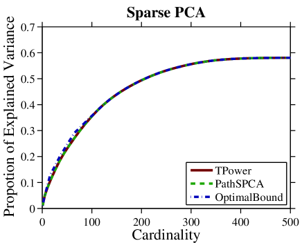
(a) Colon Cancer

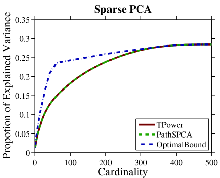
(b) Lymphoma

Figure 4.1: The synthetic dataset and outlier removal result. For better viewing, please see the original pdf file.

4.1.7 Results on Document Data

In this section we evaluate the practical performance of TPower for key terms extraction on a document dataset 20 Newsgroups (20NG). The 20NG  is a dataset collected and originally used for document classification by Lang (1995). A total number of $18,846$ documents, evenly distributed across 20 classes, are left after removing duplicates and newsgroup-identifying headers. This corpus contains $26,214$ distinct terms after stemming and stop word removal. Each document is then represented as a term-frequency vector and normalized to one. We use the top 1,000 terms according to the DF (document frequency) of the terms in the corpus. We extract 5 sparse PCs on this dataset. The cardinality setting for the 5 sparse PCs is 20-20-10-10-10. Table 4.5 lists the terms associated with the 1st, 2nd and 5th sparse PCs. The interpretation is quite clear: the 1st sparse PC is about figures, the 2nd is about computer science, and the 5th is on religion. We have observed that quite similar terms are extracted by PathSPCA under the same cardinality setting. Here we do not list the 3rd and 4th PCs since they overlap with the listed ones due to the non-orthogonality of sparse PCs.

Table 4.5: Terms associated with the first 1st, 2nd, 5th sparse PCs. Dataset: 20NG.

1st PC (20 terms)	2nd PC (20 terms)	5th PC (10 terms)
“1”	“edu”	“dont”
“2”	“system”	“time”
“3”	“inform”	“people”
“4”	“includ”	“believ”
“5”	“support”	“god”
“10”	“program”	“exist”
“20”	“version”	“christan”
“15”	“set”	“jesus”
“8”	“window”	“christ”
“6”	“softwar”	“atheist”
“16”	“avail”
“12”	“file”
“14”	“data”
“7”	“user”
“18”	“grafic”
“9”	“color”
“13”	“imag”
“11”	“displai”
“0”	“format”
“la”	“ftp”

4.1.8 Summary

To summarize this group of experiments on sparse PCA, the basic finding is that TPower performs quite competitively in terms of the trade-off between explained variance and representation sparsity. The performance is comparable to PathSPCA (d’Aspremont et al., 2008) and GPower (Journée et al., 2010) both on the synthetic and on the real datasets. It is observed that TPower, PathSPCA and GPower outperform SPCA (Zou et al., 2006) on the benchmark data Pitprops. Although performing quite similarly, TPower, PathSPCA and GPower are different algorithms: TPower is a power iteration method while PathSPCA is a greedy forward selection method, both directly address the cardinality constrained sparse eigenvalue problem (1.1), while GPower is a power iteration method for certain regularized versions of sparse eigenvalue problem (see the previous Section 4.1.1). While strong theoretical guarantee can be established for the TPower method, it remains open to show that PathSPCA and GPower have a similar sparse recovery performance.

4.2 Densest $k$-Subgraph Finding

As another concrete application, we show that with proper modification, TPower can be applied to the densest $k$-subgraph finding problem. Given an undirected graph $G=(V,E)$, $|V|=n$, and integer $1\leq k\leq n$, the densest $k$-subgraph (DkS) problem is to find a set of $k$ vertices with maximum average degree in the subgraph induced by this set. In the weighted version of DkS we are also given nonnegative weights on the edges and the goal is to find a $k$-vertex induced subgraph of maximum average edge weight. Algorithms for finding DkS are useful tools for analyzing networks. In particular, they have been used to select features for ranking (Geng et al., 2007), to identify cores of communities (Kumar et al., 1999), and to combat link spam (Gibson et al., 2005).

It has been shown that the DkS problem is NP hard for bipartite graphs and chordal graphs (Corneil & Perl, 1984), and even for graphs of maximum degree three (Feige et al., 2001). A large body of algorithms have been proposed based on a variety of techniques including greedy algorithms (Feige et al., 2001; Asahiro et al., 2002; Ravi et al., 1994), linear programming (Billionnet & Roupin, 2004; Khuller & Saha, 2009), and semidefinite programming (Srivastav & Wolf, 1998; Ye & Zhang, 2003). For general $k$, the algorithm developed by Feige et al. (2001) achieves the best approximation ratio of $O(n^{\epsilon})$ where $\epsilon<1/3$. Ravi et al. (1994) proposed 4-approximation algorithms for weighted DkS on complete graphs for which the weights satisfy the triangle inequality. Liazi et al. (2008) has presented a 3-approximation algorithm for DkS for chordal graphs. Recently, Jiang et al. (2010) proposed to reformulate DkS as a 1-mean clustering problem and developed a $2$-approximation to the reformulated clustering problem. Moreover, based on this reformulation, Yang (2010) proposed a $1+\epsilon$-approximation algorithm with certain exhaustive (and thus expensive) initialization procedure. In general, however, Khot (2006) showed that DkS has no polynomial time approximation scheme (PTAS), assuming that there are no sub-exponential time algorithms for problems in NP.

Mathematically, DkS can be restated as the following binary quadratic programming problem:

$$\max_{\pi\in\mathbb{R}^{n}}\pi^{\top}W\pi,\ \ \ \ \ \ \ \text{subject to }\pi\in\{1,0\}^{n},\|\pi\|_{0}=k,$$ (4.3)

where $W$ is the (non-negative weighted) adjacency matrix of $G$. If $G$ is an undirected graph, then $W$ is symmetric. If $G$ is directed, then $A$ could be asymmetric. In this latter case, from the fact that $\pi^{\top}W\pi=\pi^{\top}\frac{W+W^{\top}}{2}\pi$, we may equivalently solve Problem (4.3) by replacing $W$ with $\frac{W+W^{\top}}{2}$. Therefore, in the following discussion, we always assume that the affinity matrix $W$ is symmetric (or $G$ is undirected).

4.2.1 The TPower-DkS Algorithm

We propose the TPower-DkS algorithm as a slight modification of TPower, to solve the DkS problem. The process generates a sequence of intermediate vectors $\pi_{0},\pi_{1},...$ from a starting vector $\pi_{0}$. At each step $t$ the vector $\pi_{t-1}$ is multiplied by the matrix $W$, then $\pi_{t}$ is set to be the indicator vector of the top $k$ entries in $W\pi_{t-1}$. The TPower-Dks is formally given in Algorithm 2.

Input : $W\in\mathbb{S}^{n}_{+}$,, initial vector $\pi_{0}\in\mathbb{R}^{n}$

Output : $\pi_{t}$

Parameters : cardinality $k\in\{1,...,n\}$

Let $t=1$.

repeat

      

      Compute $\pi^{\prime}_{t}=W\pi_{t-1}$.

      Identify $F_{t}=\text{supp}(\pi^{\prime}_{t},k)$ the index set of $\pi^{\prime}_{t}$ with top $k$ values.

      Set $\pi_{t}$ to be 1 on the index set $F_{t}$, and 0 otherwise.

      $t\leftarrow t+1$.

until Convergence;

Algorithm 2 Truncated Power Method for DkS (TPower-DkS)

Remark 4.

By relaxing the constraint $\pi\in\{0,1\}^{n}$ to $\|\pi\|=\sqrt{k}$, we may convert the densest $k$-subgraph problem (4.3) to the standard sparse eigenvalue problem (1.1) (up to a scaling) and then directly apply TPower (in Algorithm 1) for solution. Our numerical experience shows that such a relaxation strategy also works satisfactory in practice, although is slightly inferior to TPower-DkS (in Algorithm 2) which directly addresses the original problem.

Note that in Algorithm 2 we require that $W$ is positive semidefinite. The motivation of this requirement is to guarantee the convexity of the objective in problem (4.3), and thus following the similar arguments in (Journée et al., 2010) it can be shown that the objective value will be monotonically increasing during the iterations. In many real-world DkS problems, however, it is often the case that the affinity matrix $W$ is not positive semi-definite. In this case, the objective is non-convex and thus the monotonicity of TPower-DkS does not hold. However, this complication can be circumvented by instead running the algorithm with the shifted quadratic function:

$$\max_{\pi\in\mathbb{R}^{n}}\pi^{\top}(W+\tilde{\lambda}I_{p\times p})\pi,\ \ \ \text{subject to }\pi\in\{0,1\}^{n},\|\pi\|_{0}=k.$$

where $\tilde{\lambda}>0$ is large enough such that $\tilde{W}=W+\tilde{\lambda}I_{p\times p}\in\mathbb{S}^{n}_{+}$. On the domain of interest, this change only adds a constant term to the objective function. The TPower-DkS, however, produces a different sequence of iterates, and there is a clear trade-off. If the second term dominates the first term (say by choosing a very large $\tilde{\lambda}$), the objective function becomes approximately a squared norm, and the algorithm tends to terminate in very few iterations. In the limiting case of $\tilde{\lambda}\to\infty$, the method will not move away from the initial iterate. To handle this issue, we propose to gradually increase $\tilde{\lambda}$ during the iterations and we do so only when the monotonicity is violated. To be precise, if at a time instance $t$, $\pi_{t}^{\top}W\pi_{t}<\pi_{t-1}^{\top}W\pi_{t-1}$, then we add $\tilde{\lambda}I_{p\times p}$ to $W$ with a gradually increased $\tilde{\lambda}$ by repeating the current iteration with the updated matrix until $\pi_{t}^{\top}(W+\tilde{\lambda}I_{p\times p})\pi_{t}\geq\pi_{t-1}^{\top}(W+\lambda I_{p\times p})\pi_{t-1}$ , which implies $\pi_{t}^{\top}W\pi_{t}\geq\pi_{t-1}^{\top}W\pi_{t-1}$.

4.2.2 On Initialization

Since TPower-DkS is a monotonically increasing procedure, it guarantees to improve the initial point $\pi_{0}$. Basically, any existing approximation DkS method, e.g., greedy algorithms (Feige et al., 2001; Ravi et al., 1994), can be used to initialize TPower-DkS. In our numerical experiments, we observe that by simply setting $\pi_{0}$ as the indicator vector of the vertices with the top $k$ (weighted) degrees, our method can achieve very competitive results on all the real-world datasets we have tested on.

4.2.3 Results on Web Graphs

We have tested TPower on four page-level web graphs: cnr-2000, amazon-2008, ljournal-2008, hollywood-2009, from the WebGraph framework provided by the Laboratory for Web Algorithms . We treated each directed arc as an undirected edge. Table 4.6 lists the statistics of the datasets used in the experiment.

Table 4.6: The statistics of the web graph datasets.

Graph	Nodes ($|V|$)	Total Arcs ($|E|$)	Average Degree
cnr-2000	325,557	3,216,152	9.88
amazon-2008	735,323	5,158,388	7.02
ljournal-2008	5,363,260	79,023,142	14.73
hollywood-2009	1,139,905	113,891,327	99.91

We compare our TPower-DkS method with two greedy methods for the DkS problem. One greedy method is proposed by Ravi et al. (1994) which is referred to as Greedy-Ravi in our experiments. The Greedy-Ravi algorithm works as follows: it starts from a heaviest edge and repeatedly adds a vertex to the current subgraph to maximize the weight of the resulting new subgraph; this process is repeated until $k$ vertices are chosen. The other greedy method is developed by Feige et al. (2001, Procedure 2) which is referred as Greedy-Feige in our experiments. The procedure works as follows: let $S$ denote the $k/2$ vertices with the highest degrees in $G$; let $C$ denote the $k/2$ vertices in the remaining vertices with largest number of neighbors in $S$; return $S\cup C$.

Figure 4.2 shows the density value $\pi^{\top}W\pi/k$ and CPU time versus the cardinality $k$. From the density curves we can observe that on cnr-2000, ljournal-2008 and hollywood-2009, TPower-DkS consistently outputs denser subgraphs than the two greedy algorithms, while on amazon-2008, TPower-DkS and Greedy-Ravi are comparable and both are better than Greedy-Feige. For CPU running time, it can be seen from the right column of Figure 4.2 that Greedy-Feige is the fastest among the three methods while TPower-DkS is only slightly slower. This is due to the fact that TPower-DkS needs iterative matrix-vector products while Greedy-Feige only needs a few degree sorting outputs. Although TPower-DkS is slightly slower than Greedy-Feige, it is still quite efficient. For example, on hollywood-2009 which has hundreds of millions of arcs, for each $k$, Greedy-Feige terminates within about 1 second while TPower terminates within about 10 seconds. The Greedy-Ravi method is however much slower than the other two on all the graphs when $k$ is large.

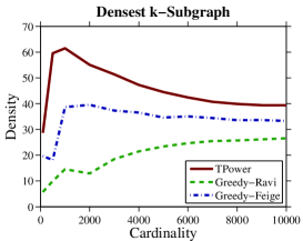
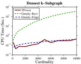
(a) cnr-2000

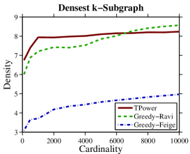
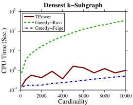
(b) amazon-2008

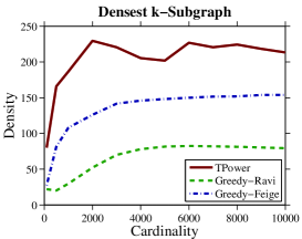
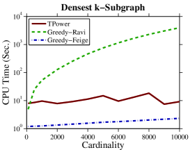
(c) ljournal-2008

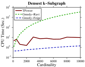
(d) hollywood-2009

Figure 4.2: Identifying densest $k$-subgraph on four web graphs. Left: density curves as a function of $k$. Right: CPU time curves as a function of $k$.

4.2.4 Results on Air-Travel Routine

We have applied TPower-DkS to identify subsets of American and Canadian cities that are most easily connected to each other, in terms of estimated commercial airline travel time. The graph  is of size $|V|=456$ and $|E|=71,959$: the vertices are $456$ busiest commercial airports in United States and Canada, while the weight $w_{ij}$ of edge $e_{ij}$ is set to the inverse of the mean time it takes to travel from city $i$ to city $j$ by airline, including estimated stopover delays. Due to the headwind effect, the transit time can depend on the direction of travel; thus $36\%$ of the weight are asymmetric. Figure 3(a) shows a map of air-travel routine.

As in the previous experiment, we compare TPower-DkS to Greedy-Ravi and Greedy-Feige on this dataset. For all the three algorithms, the densities of $k$-subgraphs under different $k$ values are shown in Figure 3(b), and the CPU running time curves are given in Figure 3(c). From the former figure we observe that TPower-DkS consistently outperforms the other two greedy algorithms in terms of the density of the extracted $k$-subgraphs. From the latter figure we can see that TPower-DkS is slightly slower than Greed-Feige but much faster than Greedy-Ravi. Figure 3(d),3(e), and 3(f) illustrate the densest $k$-subgraph with $k=30$ outputted by the three algorithms. In each of these three subgraph, the red dot indicates the representing city with the largest (weighted) degree. Both TPower-DkS and Greedy-Feige reveal 30 cities in east US. The former takes Cleveland as the representing city while the latter Cincinnati. Greedy-Ravi reveals 30 cities in west US and CA and takes Vancouver as the representing city. Visual inspection shows that the subgraph recovered by TPower-DkS is the densest among the three.

After discovering the densest $k$-subgraph, we can eliminate their nodes and edges from the graph and then apply the algorithms on the reduced graph to search for the next densest subgraph. Such a sequential procedure can be repeated to find multiple densest $k$-subgraphs. Figure 3(g),3(h), and 3(i) illustrate sequentially estimated six densest $30$-subgraphs by the three algorithms. Again, visual inspection shows that our method output more geographically compact subsets of cities than the other two. As a quantitative result, the total density of the six subgraphs discovered by the three algorithms is: 1.14 (TPower-DkS), 0.90 (Greedy-Feige) and 0.99 (Greedy-Ravi), respectively.

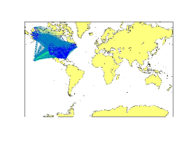
(a) The air-travel route map

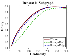
(b) Density

(c) CPU Time

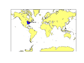
(d) TPower-DkS

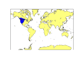
(e) Greedy-Ravi

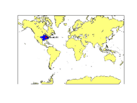
(f) Greedy-Feige

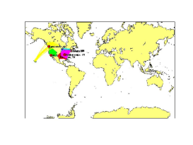
(g) TPower-DkS

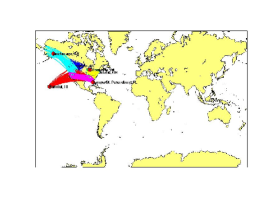
(h) Greedy-Ravi

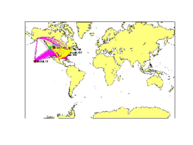
(i) Greedy-Feige

Figure 4.3: Identifying densest $k$-subgraph of air-travel routing. Row 1: Route map, and the density and CPU time evolving curves. Row 2: The densest $30$-subgraph discovered by the three algorithms. Row 3: Sequentially discovered six densest $30$-subgraph by the three algorithms.

5 Conclusion and Future Work

The sparse eigenvalue problem has been widely studied in machine learning with applications such as sparse PCA. TPower is a truncated power iteration method that approximately solves the nonconvex sparse eigenvalue problem. Our analysis shows that when the underlying matrix has sparse eigenvectors, under proper conditions TPower can approximately recover the true sparse solution. The theoretical benefit of this method is that with appropriate initialization, the reconstruction quality depends on the restricted matrix perturbation error at size $s$ that is comparable to the sparsity $\bar{k}$, instead of the full matrix dimension $p$. This explains why this method has good empirical performance. To our knowledge, this is the first theoretical result of this kind, although our empirical study suggests that it might be possible to prove related sparse recovery results for some other algorithms we have tested.

We have applied TPower to two concrete applications: sparse PCA and the densest $k$-subgraph finding problem. Extensive experimental results on synthetic and real-world datasets validate the effectiveness and efficiency of the TPower algorithm.

Appendix A Proof of Theorem 1

We state the following standard result from the perturbation theory of symmetric eigenvalue problem. It can be found for example in (Golub & Van Loan, 1996).

Lemma 1.

If $B$ and $B+U$ are $p\times p$ symmetric matrices, then $\forall 1\leq k\leq p$,

$$\lambda_{k}(B)+\lambda_{p}(U)\leq\lambda_{k}(B+U)\leq\lambda_{k}(B)+\lambda_{1}(U),$$

where $\lambda_{k}(B)$ denotes the $k$-th largest eigenvalue of matrix $B$.

Lemma 2.

Consider set $F$ such that $\text{supp}(\bar{x})\subseteq F$ with $|F|=s$. If $\rho(E,s)\leq\Delta\lambda/2$, then the ratio of the second largest (in absolute value) to the largest eigenvalue of sub matrix $A_{F}$ is no more than $\gamma(s)$. Moreover,

$$\|\bar{x}^{\top}-x(F)\|\leq\delta(s):=\frac{\sqrt{2}\rho(E,s)}{\sqrt{\rho(E,s)^{2}+(\Delta\lambda-2\rho(E,s))^{2}}}.$$

Proof.

We may use Lemma 1 with $B=\bar{A}_{F}$ and $U=E_{F}$ to obtain

$$\lambda_{1}(A_{F})\geq\lambda_{1}(\bar{A}_{F})+\lambda_{p}(E_{F})\geq\lambda_{1}(\bar{A}_{F})-\rho(E_{F})\geq\lambda-\rho(E,s)$$

and $\forall j\geq 2$,

$$|\lambda_{j}(A_{F})|\leq|\lambda_{j}(\bar{A}_{F})|+\rho(E_{F})\leq\lambda-\Delta\lambda+\rho(E,s).$$

This implies the first statement of the lemma.

Now let $x(F)$, the largest eigenvector of $A_{F}$, be $\alpha\bar{x}+\beta x^{\prime}$, where $\|\bar{x}\|_{2}=\|x^{\prime}\|_{2}=1$, $\bar{x}^{\top}x^{\prime}=0$ and $\alpha^{2}+\beta^{2}=1$, with eigenvalue $\lambda^{\prime}\geq\lambda-\rho(E,s)$. This implies that

$$\alpha A_{F}\bar{x}+\beta A_{F}x^{\prime}=\lambda^{\prime}(\alpha\bar{x}+\beta x^{\prime}),$$

implying

$$\alpha x^{\prime\top}A_{F}\bar{x}+\beta x^{\prime\top}A_{F}x^{\prime}=\lambda^{\prime}\beta.$$

That is,

$$|\beta|=|\alpha|\frac{x^{\prime\top}A_{F}\bar{x}}{\lambda^{\prime}-x^{\prime\top}A_{F}x^{\prime}}\leq|\alpha|\frac{|x^{\prime\top}A_{F}\bar{x}|}{\lambda^{\prime}-x^{\prime\top}A_{F}x^{\prime}}=|\alpha|\frac{|x^{\prime\top}E_{F}\bar{x}|}{\lambda^{\prime}-x^{\prime\top}A_{F}x^{\prime}}\leq t|\alpha|,$$

where $t=\rho(E,s)/(\Delta\lambda-2\rho(E,s))$. This implies that $\alpha^{2}(1+t^{2})\geq\alpha^{2}+\beta^{2}=1$, and thus $\alpha^{2}\geq 1/(1+t^{2})$. Without loss of generality, we may assume that $\alpha>0$, because otherwise we can replace $\bar{x}$ with $-\bar{x}$. It follows that

$$\|x(F)-\bar{x}\|^{2}=2-2x(F)^{\top}\bar{x}=2-2\alpha\leq 2\frac{\sqrt{1+t^{2}}-1}{\sqrt{1+t^{2}}}\leq 2\frac{t^{2}}{1+t^{2}}.$$

This implies the desired bound. ∎

The following result measures the progress of untruncated power method.

Lemma 3.

Let $y$ be the eigenvector with the largest (in absolute value) eigenvalue of a symmetric matrix $A$, and let $\gamma<1$ be the ratio of the second largest to largest eigenvalue in absolute values. Given any $x$ such that $\|x\|=1$ and $y^{\top}x>0$; let $x^{\prime}=Ax/\|Ax\|$, then

$$|y^{\top}x^{\prime}|\geq|y^{\top}x|[1+(1-\gamma^{2})(1-(y^{\top}x)^{2})/2].$$

Proof.

Without loss of generality, we may assume that $\lambda_{1}(A)=1$ is the largest eigenvalue in absolute value, and $|\lambda_{j}(A)|\leq\gamma$ when $j>1$. We can decompose $x$ as $x=\alpha y+\beta y^{\prime}$, where $y^{\top}y^{\prime}=0$, $\|y\|=\|y^{\prime}\|=1$, and $\alpha^{2}+\beta^{2}=1$. Then $|\alpha|=|x^{\top}y|$. Let $z^{\prime}=Ay^{\prime}$, then $\|z^{\prime}\|\leq\gamma$ and $y^{\top}z^{\prime}=0$. This means $Ax=\alpha y+\beta z^{\prime}$, and

$$|y^{\top}x^{\prime}|= \frac{|y^{\top}Ax|}{\|Ax\|}=\frac{|\alpha|}{\sqrt{\alpha^{2}+\beta^{2}\|z^{\prime}\|^{2}}}\geq\frac{|\alpha|}{\sqrt{\alpha^{2}+\beta^{2}\gamma^{2}}}$$

$$= \frac{|y^{\top}x|}{\sqrt{1-(1-\gamma^{2})(1-(y^{\top}x)^{2})}}$$

$$\geq |y^{\top}x|\;[1+(1-\gamma^{2})(1-(y^{\top}x)^{2})/2].$$

The last inequality is due to $1/\sqrt{1-z}\geq 1+z/2$ for $z\in[0,1)$. This proves the desired bound. ∎

Lemma 4.

Consider $\bar{x}$ with $\text{supp}(\bar{x})=\bar{F}$ and $\bar{k}=|\bar{F}|$. Consider $y$ and let $F=\text{supp}(y,k)$ be the indices of $y$ with the largest $k$ absolute values. If $\|\bar{x}\|=\|y\|=1$, then

$$|\text{Truncate}(y,F)^{\top}\bar{x}|\geq|y^{\top}\bar{x}|-(\bar{k}/k)^{1/2}\min\left[1,(1+(\bar{k}/k)^{1/2})\;(1-(y^{\top}\bar{x})^{2})\right].$$

Proof.

Without loss of generality, we assume that $y^{\top}\bar{x}=\Delta>0$. We can also assume that $\Delta\geq\sqrt{\bar{k}/(\bar{k}+k)}$ because otherwise the right hand side is smaller than zero, and thus the result holds trivially.

Let $F_{1}=\bar{F}\setminus F$, and $F_{2}=\bar{F}\cap F$, and $F_{3}=F\setminus\bar{F}$. Now, let $\bar{\alpha}=\|\bar{x}_{F_{1}}\|$, $\bar{\beta}=\|\bar{x}_{F_{2}}\|$, $\alpha=\|y_{F_{1}}\|$, $\beta=\|y_{F_{2}}\|$, and $\gamma=\|y_{F_{3}}\|$. let $k_{1}=|F_{1}|$, $k_{2}=|F_{2}|$, and $k_{3}=|F_{3}|$. It follows that $\alpha^{2}/k_{1}\leq\gamma^{2}/k_{3}$. Therefore

$$\Delta^{2}\leq[\bar{\alpha}\alpha+\bar{\beta}\beta]^{2}\leq\alpha^{2}+\beta^{2}\leq 1-\gamma^{2}\leq 1-(k_{3}/k_{1})\alpha^{2}.$$

This implies that

$$\alpha^{2}\leq(k_{1}/k_{3})(1-\Delta^{2})\leq(\bar{k}/k)(1-\Delta^{2})\leq\Delta^{2},$$ (A.1)

where the second inequality follows from $\bar{k}<k$ and the last inequality follows from the assumption $\Delta\geq\sqrt{\bar{k}/(\bar{k}+k)}$. Now by solving the following inequality for $\bar{\alpha}$:

$$\alpha\bar{\alpha}+\sqrt{1-\alpha^{2}}\sqrt{1-\bar{\alpha}^{2}}\geq\alpha\bar{\alpha}+\beta\bar{\beta}\geq\Delta\geq\alpha\geq\alpha\bar{\alpha},$$

we obtain that

$$\bar{\alpha}\leq\alpha\Delta+\sqrt{1-\alpha^{2}}\sqrt{1-\Delta^{2}}\leq\min\left[1,\alpha+\sqrt{1-\Delta^{2}}\right]\leq\min\left[1,(1+(\bar{k}/k)^{1/2})\sqrt{1-\Delta^{2}}\right],$$ (A.2)

where the second inequality follows from the Cauchy-Schwartz inequality and $\Delta\leq 1$, $\sqrt{1-\alpha^{2}}\leq 1$, while the last inequality follows from (A.1). Finally,

$$|y^{\top}\bar{x}|-|\text{Truncate}(y,F)^{\top}\bar{x}| \leq |(y-\text{Truncate}(y,F))^{\top}\bar{x}|$$

$$\leq \alpha\bar{\alpha}\leq(\bar{k}/k)^{1/2}\min\left[1,(1+(\bar{k}/k)^{1/2})\;(1-(y^{\top}\bar{x})^{2})\right],$$

where the last inequality follows from (A.1) and (A.2). This leads to the desired bound. ∎

Next is our main lemma, which says each step of sparse power method improves eigenvector estimation.

Lemma 5.

Let $s=2k+\bar{k}$. We have

$$|\hat{x}_{t}^{\top}\bar{x}|\geq(|x^{\top}_{t-1}\bar{x}|-\delta(s))[1+(1-\gamma(s)^{2})(1-(|x^{\top}_{t-1}\bar{x}|-\delta(s))^{2})/2]-\delta(s)-(\bar{k}/k)^{1/2}.$$

If $|x_{t-1}^{\top}\bar{x}|>1/\sqrt{3}+\delta(s)$, then

$$\sqrt{1-|\hat{x}_{t}^{\top}\bar{x}|}\leq\mu_{2}\sqrt{1-|x_{t-1}^{\top}\bar{x}|}+\sqrt{5}\delta(s).$$

Proof.

Let $F=F_{t-1}\cup F_{t}\cup\text{supp}(\bar{x})$. Consider the following vector

$$\tilde{x}^{\prime}_{t}=A_{F}x_{t-1}/\|A_{F}x_{t-1}\|,$$ (A.3)

where $A_{F}$ denotes the restriction of $A$ on the rows and columns indexed by $F$. We note that replacing $x^{\prime}_{t}$ with $\tilde{x}^{\prime}_{t}$ in Algorithm 2 does not affect the output iteration sequence $\{x_{t}\}$ because of the sparsity of $x_{t-1}$ and the fact that the truncation operation is invariant to scaling. Therefore for notation simplicity, in the following proof we will simply assume that $x^{\prime}_{t}$ is redefined as $x^{\prime}_{t}=\tilde{x}^{\prime}_{t}$ according to (A.3).

Based on the above notation, we have

$$|x^{\prime\top}_{t}x(F)| \geq |x_{t-1}^{\top}x(F)|[1+(1-\gamma(s)^{2})(1-(x_{t-1}^{\top}x(F))^{2})/2]$$

$$\geq (|x^{\top}_{t-1}\bar{x}|-\delta(s))[1+(1-\gamma(s)^{2})(1-(|x^{\top}_{t-1}\bar{x}|-\delta(s))^{2})/2],$$

where the first inequality follows from Lemma 3, and the second is from Lemma 2 and $|x_{t-1}^{\top}\bar{x}|\geq|x^{\top}_{t-1}x(F)|-\delta(s)$, and the fact that $x(1+(1-\gamma^{2})(1-x^{2})/2)$ is increasing when $x\in[0,1]$. We can now use Lemma 2 again, and the preceding inequality implies that

$$|x^{\prime\top}_{t}\bar{x}|\geq(|x^{\top}_{t-1}\bar{x}|-\delta(s))[1+(1-\gamma(s)^{2})(1-(|x^{\top}_{t-1}\bar{x}|-\delta(s))^{2})/2]-\delta(s).$$

Next we can apply Lemma 4 to obtain

$$|\hat{x}_{t}^{\top}\bar{x}| \geq |{x^{\prime}_{t}}^{\top}\bar{x}|-(\bar{k}/k)^{1/2}$$

$$\geq (|x^{\top}_{t-1}\bar{x}|-\delta(s))[1+(1-\gamma(s)^{2})(1-(|x^{\top}_{t-1}\bar{x}|-\delta(s))^{2})/2]-\delta(s)-(\bar{k}/k)^{1/2}.$$

This leads to the first desired inequality.

Next we will prove the second inequality. Without loss of generality and for simplicity, we may assume that $x^{\prime\top}_{t}x(F)\geq 0$ and $x_{t-1}^{\top}\bar{x}\geq 0$, because otherwise we can simply do appropriate sign changes in the proof. We obtain from Lemma 3 that

$$x^{\prime\top}_{t}x(F)\geq x_{t-1}^{\top}x(F)\;[1+(1-\gamma(s)^{2})(1-(x_{t-1}^{\top}x(F))^{2})/2].$$

This implies that

$$[1-x^{\prime\top}_{t}x(F)]\leq [1-x_{t-1}^{\top}x(F)]\;[1-(1-\gamma(s)^{2})(1+x_{t-1}^{\top}x(F))(x_{t-1}^{\top}x(F))/2]$$

$$\leq [1-x_{t-1}^{\top}x(F)]\;[1-0.45(1-\gamma(s)^{2})],$$

where in the derivation of the second inequality, we have used Lemma 2 and the assumption of the lemma that implies $x_{t-1}^{\top}x(F)\geq x_{t-1}^{\top}\bar{x}-\delta(s)\geq 1/\sqrt{3}$. We thus have

$$\|x^{\prime}_{t}-x(F)\|\leq\|x_{t-1}-x(F)\|\;\sqrt{1-0.45(1-\gamma(s)^{2})}.$$

Therefore using Lemma 2, we have

$$\|x^{\prime}_{t}-\bar{x}\|\leq\|x_{t-1}-\bar{x}\|\;\sqrt{1-0.45(1-\gamma(s)^{2})}+2\delta(s).$$

This is equivalent to

$$\sqrt{1-|{x^{\prime}_{t}}^{\top}\bar{x}|}\leq\sqrt{1-|x_{t-1}^{\top}\bar{x}|}\sqrt{1-0.45(1-\gamma(s)^{2})}+\sqrt{2}\delta(s).$$

Next we can apply Lemma 4 and use $\bar{k}/k\leq 0.25$ to obtain

$$\sqrt{1-|\hat{x}_{t}^{\top}\bar{x}|} \leq \sqrt{1-|{x^{\prime}_{t}}^{\top}\bar{x}|+((\bar{k}/k)^{1/2}+\bar{k}/k)(1-|{x^{\prime}_{t}}^{\top}\bar{x}|^{2})}$$

$$\leq \sqrt{1-|{x^{\prime}_{t}}^{\top}\bar{x}|}\sqrt{1+3(\bar{k}/k)^{1/2}}$$

$$\leq \mu_{2}\sqrt{1-|{x_{t-1}}^{\top}\bar{x}|}+\sqrt{5}\delta(s).$$

This proves the second desired inequality. ∎

Proof of Theorem 1

We know if $|x_{t-1}^{\top}\bar{x}|\geq u+\delta(s)$, then Lemma 5 implies:

$$|\hat{x}_{t}^{\top}\bar{x}|\geq (|x_{t-1}^{\top}\bar{x}|-\delta(s))[1+(1-\gamma(s)^{2})(1-(|x_{t-1}^{\top}\bar{x}|-\delta(s))^{2})/2]-(\delta(s)+(\bar{k}/k)^{1/2})$$

$$\geq u[1+(1-\gamma(s)^{2})(1-u^{2})/2]-(\delta(s)+(\bar{k}/k)^{1/2})\geq u+\delta(s).$$

The first inequality uses Lemma 5; the second inequality uses $z(1+(1-\gamma^{2})(1-z^{2})/2)$ is an increasing function of $z\in[0,1]$; and the third inequality uses the assumption of $u$ in the theorem. This implies (by an easy induction argument) that we have $|\hat{x}_{t}^{\top}\bar{x}|\geq u+\delta$ for all $t\geq 0$.

Now we can prove the theorem by induction. The bound clearly holds at $t=0$. Assume it holds at some $t-1$. If we have $|\hat{x}_{t-1}^{\top}\bar{x}|\leq 1/\sqrt{3}+\delta(s)$, then since $z(1-z^{2})$ is increasing in $[0,1/\sqrt{3}]$, and from Lemma 5 we have

$$|\hat{x}_{t}^{\top}\bar{x}|\geq (|x_{t-1}^{\top}\bar{x}|-\delta(s))[1+(1-\gamma(s)^{2})(1-(|x_{t-1}^{\top}\bar{x}|-\delta(s))^{2})/2-(\delta(s)+(\bar{k}/k)^{1/2})$$

$$\geq |x_{t-1}^{\top}\bar{x}|-\delta(s)+(1-\gamma(s)^{2})u(1-u^{2})/2-(\delta(s)+(\bar{k}/k)^{1/2})$$

$$\geq |x_{t-1}^{\top}\bar{x}|+\mu_{1}.$$

Combing this inequality with $|x_{t}^{\top}\bar{x}|=|\hat{x}_{t}^{\top}\bar{x}|/\|\hat{x}_{t}\|\geq|\hat{x}_{t}^{\top}\bar{x}|$ we get

$$1-|x_{t}^{\top}\bar{x}|\leq 1-|\hat{x}_{t}^{\top}\bar{x}|\leq(1-\mu_{1})[1-|x_{t-1}^{\top}\bar{x}|],$$

which implies the theorem at $t$.

If $|\hat{x}_{t-1}^{\top}\bar{x}|\geq 1/\sqrt{3}+\delta(s)$, then we have from Lemma 5

$$\sqrt{1-|x_{t}^{\top}\bar{x}|}\leq\sqrt{1-|\hat{x}_{t}^{\top}\bar{x}|}\leq\mu_{2}\sqrt{1-|x_{t-1}^{\top}\bar{x}|}+\sqrt{5}\delta(s),$$

which implies the theorem at $t$. This finishes induction.

References

- Alizadeh et al. (2000) Alizadeh, A., Eisen, M., Davis, R., Ma, C., Lossos, I., and Rosenwald, A. Distinct types of diffuse large b-cell lymphoma identified by gene expression profiling. Nature, 403:503–511, 2000.
- Alon et al. (1999) Alon, A., Barkai, N., Notterman, D. A., Gish, K., Ybarra, S., Mack, D., and Levine, A. J. Broad patterns of gene expression revealed by clustering analysis of tumor and normal colon tissues probed by oligonucleotide arrays. Cell Biology, 96:6745–6750, 1999.
- Amini & Wainwright (2009) Amini, A. A. and Wainwright, M. J. High-dimensional analysis of semidefinite relaxiation for sparse principal components. Annals of Statistics, 37:2877–2921, 2009.
- Asahiro et al. (2002) Asahiro, Y., Hassin, R., and Iwama, K. Complexity of finidng dense subgraphs. Discrete Appl. Math., 211(1-3):15–26, 2002.
- Billionnet & Roupin (2004) Billionnet, A. and Roupin, F. A deterministic algorithm for the densest k-subgraph problem using linear programming. Technical report, Technical Report, No. 486, CEDRIC, CNAM-IIE, Paris, 2004.
- Candes & Tao (2005) Candes, Emmanuel J. and Tao, Terence. Decoding by linear programming. IEEE Trans. on Information Theory, 51:4203–4215, 2005.
- Corneil & Perl (1984) Corneil, D. G. and Perl, Y. Clustering and domination in perfect graphs. Discrete Appl. Math., 9:27–39, 1984.
- d’Aspremont et al. (2007) d’Aspremont, A., Ghaoui, L. El, Jordan, M. I., and Lanckriet, G. R. G. A direct formulation for sparse pca using semidefinite programming. Siam Review, 49:434–448, 2007.
- d’Aspremont et al. (2008) d’Aspremont, A., Bach, F., and Ghaoui, L. El. Optimal solutions for sparse principal component analysis. Journal of Machine Learning Research, 9:1269–1294, 2008.
- Feige et al. (2001) Feige, U., Kortsarz, G., and Peleg, D. The dense -subgraph problem. Algorithmica, 29(3):410–421, 2001.
- Geng et al. (2007) Geng, X., Liu, T., Qin, T., and Li, H. Feature selection for ranking. In Proceedings of SIGIR’07, 2007.
- Gibson et al. (2005) Gibson, D., Kumar, R., and Tomkins, A. Discovering large dense subgraphs in massive graphs. In Proceedings of the 31st International Conference on Very Large Data Bases (VLDB 05), pp. 721–732, 2005.
- Golub & Van Loan (1996) Golub, G.H. and Van Loan, C.F. Matrix computations. Johns Hopkins University Press, Baltimore, MD, third edition, 1996.
- Horn & Johnson (1991) Horn, R.A. and Johnson, C.R. Topics in Matrix Analysis. Canbridge University Press, 1991.
- Jeffers (1967) Jeffers, J. Two case studies in the application of principal components. Applied Statistics, pp. 225–236, 1967.
- Jiang et al. (2010) Jiang, P., Peng, J., Heath, M., and Yang, R. Finding densest k-subgraph via 1-mean clustering and low-dimension approximation. Technical report, 2010.
- Johnstone (2001) Johnstone, I. M. On the distribution of the largest eigenvalue in principal components analysis. Annals of Statistics, 29:295–327, 2001.
- Jolliffe et al. (2003) Jolliffe, I. T., Trendafilov, N. T., and Uddin, M. A modified principal component technique based on the lasso. J. Comput.Graph.Statist., pp. 531–547, 2003.
- Journée et al. (2010) Journée, Michel, Nesterov, Yurii, Richtárik, Peter, and Sepulchre, Rodolphe. Generalized power method for sparse principal component analysis. Journal of Machine Learning Research, 11:517–553, 2010.
- Khot (2006) Khot, S. Ruling out ptas for graph min-bisection, dense k-subgraph, and bipartite clique. SIAM J. Comput., 36(4):1025–1071, 2006.
- Khuller & Saha (2009) Khuller, S. and Saha, B. On finding dense subgraphs. In Proceedings of the 36th International Colloquium on Automata, Languages and Programming (ICALP’09), pp. 597–608, 2009.
- Kumar et al. (1999) Kumar, R., Raghavan, P., Rajagopalan, S., and Tomkins, A. Trawling the web for emerging cyber-communities. In Proceedings of the 8th World Wide Web Conference (WWW’99), pp. 403–410, 1999.
- Lang (1995) Lang, K. Newsweeder: Leanring to filter netnews. In International Conference on Machine Learning, pp. 331–339, 1995.
- Liazi et al. (2008) Liazi, M., Milis, I., and Zissimopoulos, V. A constant approximation algorithm for the densest k-subgraph problem on chordal graphs. Information Processing Letters, 108(1):29–32, 2008.
- Mackey (2008) Mackey, L. Deflation methods for sparse pca. In NIPS, 2008.
- Moghaddam et al. (2006) Moghaddam, B., Weiss, Y., and Avidan, S. Generalized spectral bounds for sparse lda. In ICML, pp. 641–648, 2006.
- Ravi et al. (1994) Ravi, S. S., Rosenkrantz, D. J., and Tayi, G. K. Heuristic and special case algorithms for dispersion problems. Oper. Res., 42:299–310, 1994.
- Shen & Huang (2008) Shen, H. and Huang, J. Z. Sparse principal component analysis via regularized low rank matrix approximation. Journal of Multivariate Analysis, 99(6):1015–1034, 2008.
- Srivastav & Wolf (1998) Srivastav, A. and Wolf, K. Finding dense subgraphs with semidefinite programming. In Proc. International Workshop Approx., pp. 181–191, 1998.
- Tibshirani (1996) Tibshirani, R. Regression shrinkage and selection via the lasso. Journal of the Royal Statistical Society. Series B, 58:267–288, 1996.
- Yang (2010) Yang, R. New approximation methods for solving binary quadratic programming problem. Technical report, Master Thesis, Department of Industrial and Enterprise Systems Engineering, University of Illnois at Urbana-Champaign, 2010.
- Ye & Zhang (2003) Ye, Y. Y. and Zhang, J. W. Approximation of dense-n/2-subgraph and the complement of min-bisection. J. Global Optimization, 25:55–73, 2003.
- Zou et al. (2006) Zou, H., Hastie, T., and Tibshirani, R. Sparse principal component analysis. Journal of Computational and Graphical Statistics, 15(2):265–286, 2006.