Abstract

We present a rigorous and rather self-contained analysis of the Verdet constant in graphene-like materials. We apply the gauge-invariant magnetic perturbation theory to a nearest-neighbour tight-binding model and obtain a relatively simple and exactly computable formula for the Verdet constant, at all temperatures and all frequencies of sufficiently large absolute value. Moreover, for the standard nearest neighbour tight-binding model of graphene we show that the transverse component of the conductivity tensor has an asymptotic Taylor expansion in the external magnetic field where all the coefficients of even powers are zero.

1 Introduction

Faraday rotation is a dispersion effect discovered around 1845, which consists of the rotation of the polarization plane of a linearly polarized light-beam passing through a material in the direction of the applied magnetic field. The Faraday rotation angle $\vartheta$ is defined as

$$\vartheta=\frac{\omega d(\eta_{-}-\eta_{+})}{2c},$$

where $d$ is the thickness of the material, while $\eta_{-}$ and $\eta_{+}$ are respectively the refraction indices of the right and left circularly polarized radiation of frequency $\omega$. As we will explain in Section 1.2, if the applied magnetic field $b$ is small, then the rotation angle can be expressed as $\vartheta=d\,b\,V$ where $V$ is a constant named after Emile Verdet [1], one of the first physicists who advocated the use of Maxwell’s equations in explaining dispersion (around 1865). The Verdet constant depends on how the transverse conductivity coefficient behaves as a function of $b$ near $b=0$.

In this paper we put to work the general method proposed in [2] and apply it to the case of a tight-binding model. One advantage of a discrete model is that we can give much shorter and less technical proofs for both the thermodynamic and adiabatic limits. Another advantage is that the structure of the Bloch bands is much simpler in the discrete case, where in many interesting cases we know the exact expression of the fiber Hamiltonians, given by finite dimensional matrices.

One can relax the decay properties of the zero-field Hamiltonian, but the nearest neighbour tight-binding operator is widely used by physicists. The proofs could be carried out even for a $\mathrm{\mathbf{H}}_{0}$ with a sufficiently fast polynomial decay around the diagonal, without changing the results, but the price would be a complication of the thermodynamic limit.

1.1 A description of the Faraday effect

Let us briefly discuss the physical problem following [3] and [4]. Starting from the classical Maxwell equations, one can derive the Faraday rotation angle for a two-dimensional quasi-free electron gas placed in a magnetic field $B$ (of strength $b$) applied perpendicular to the layer. The incident light-beam is monochromatic with frequency $\omega$. The electrons are confined within a slab of thickness $d$ and move freely along the $xy$ plane. Denoting by $\left\{\sigma_{jk}^{(3\textup{D})}\right\}_{j,k=1}^{3}$ the three-dimensional conductivity tensor of the slab, and by $\sigma_{\pm}^{(3\textup{D})}=\sigma_{11}^{(3\textup{D})}\pm i\sigma_{21}^{(3\textup{D})}$, the complex refraction indexes $(\eta-i\kappa)$ for the right $(+)$ and left $(-)$ circularly polarized light are given by

$$(\eta_{\pm}-i\kappa_{\pm})^{2}=\mu\epsilon\left[1-(4\pi i/\omega\epsilon)\sigma_{\pm}^{(3\textup{D})}\right].$$ (1.1)

The element $\sigma_{33}^{(3\textup{D})}$ does not contribute to the Faraday rotation. Considering a finite thickness $d$ of the slab, the three-dimensional conductivity tensor is related to the two-dimensional conductivity tensor by the following expression

$$\sigma^{(2\textup{D})}_{jk}=\sigma^{(3\textup{D})}_{jk}\,d,\qquad j,k\in\{1,2\}.$$

Let us define the real-valued function

$$f(u,v)=\left[\left(1+\frac{4\pi}{d\omega\epsilon}u\right)^{2}+\left(\frac{4\pi}{d\omega\epsilon}v\right)^{2}\right]^{\frac{1}{4}}\cos\left(\frac{1}{2}\arctan\left[\frac{v}{\left(\frac{d\omega\epsilon}{4\pi}+u\right)}\right]\right),$$

where $\lvert u\rvert<\frac{d\omega\epsilon}{4\pi},v\in\mathbb{R}$. Now we can express $\eta_{\pm}$ appearing in expression (1.1) (to be chosen non-negative from physical considerations) as:

$$\eta_{\pm}=\sqrt{\mu\epsilon}\,f\left(\pm\sigma^{(2\textup{D})}_{21},\sigma^{(2\textup{D})}_{11}\right).$$

We are interested in studying how the Faraday angle $\vartheta$ behaves as a function of the strength of the external magnetic field, $b$. Let us assume (we will prove it later) that one can write down an asymptotic expansion of $\sigma_{jk}^{(2\textup{D})}(b)$ in powers of $b$. Moreover we assume that for the off-diagonal tensor element we have:

$$\sigma_{21}^{(2\textup{D})}(b)=b\sigma_{21}^{(1)}+\mathcal{O}(b^{2})\,,$$

while $\sigma_{11}^{(2\textup{D})}(b)$ can be expressed as:

$$\sigma_{11}^{(2\textup{D})}(b)=\sigma_{11}^{(0)}+b\sigma_{11}^{(1)}+\mathcal{O}(b^{2}).$$

Then

$$\vartheta(b)=-d\,b\,\frac{\omega\sigma_{21}^{(1)}}{c}\frac{\partial f}{\partial u}\left(0,\sigma_{11}^{(0)}\right)+\mathcal{O}(b^{2}).$$ (1.2)

Thus the Faraday rotation angle is linear in $b$ near zero, and the linear term can be put in the form $\vartheta=d\,b\,V$, where $V$ is the Verdet constant. Calculating the Verdet constant is therefore a question of finding a computable formula for the coefficient $\sigma_{21}^{(1)}$ in the asymptotic expansion of the off-diagonal conductivity element $\sigma_{21}^{(2\textup{D})}$.

The structure of our paper is as follows. In the rest of this section we introduce the mathematical notions which are necessary in order to properly define the transverse conductivity element in (1.16). In Section 2 we formulate the main result of the paper, namely Theorem 2.1. Sections 3, 4 and 5 contain the proofs of the three statements of our main theorem. In Section 6 we present our conclusions.

1.2 The configuration space

We neglect the electron-electron interactions. To simplify notation we work in a system of units where $\hbar=2m_{\rm electron}=e=1$. Let $\mbox{\boldmath$a$}_{1}=(a_{1},0)$ and $\mbox{\boldmath$a$}_{2}=(0,a_{2})$ be two vectors in $\mathbb{R}^{2}$. Define the Bravais lattice,

$$\Gamma=\{\mbox{\boldmath$\gamma$}\in\mathbb{R}^{2}\;:\;\mbox{\boldmath$\gamma$}=m\mbox{\boldmath$a$}_{1}+n\mbox{\boldmath$a$}_{2},\quad m,n\in\mathbb{Z}\}.$$

The basis $\Omega$ is modeled by $\nu_{\Omega}$ points whose position vectors are denoted by $\{\mbox{\boldmath$\underline{x}$}_{n}\}_{n=1}^{\nu_{\Omega}}$; one of them is always the origin, thus also belongs to $\Gamma$. For graphene $\nu_{\Omega}=4$ if we want to have orthogonal generating vectors of the Bravais lattice. We denote by $\lvert\Omega\rvert=\lvert a_{1}a_{2}\rvert$ the area of the unit cell (see figure 1).

The total configuration space is denoted by $\Lambda$ and describes the set of ion-core positions. A point in $\Lambda$ is called a site. Moreover, we have the identity:

$$\Lambda=\Gamma+\Omega=\{\mbox{\boldmath$\gamma$}+\mbox{\boldmath$\underline{x}$}\in\mathbb{R}^{2}\;:\;\mbox{\boldmath$\gamma$}\in\Gamma,\;\mbox{\boldmath$\underline{x}$}\in\Omega\}.$$

Define the reciprocal primitive vectors $\{\mbox{\boldmath$b$}_{n}\}_{n=1}^{\nu_{\Omega}}$ as:

$$\mbox{\boldmath$a$}_{i}\cdot\mbox{\boldmath$b$}_{j}=2\pi\delta_{ij},$$

where $\delta_{ij}$ is the Kronecker delta. The reciprocal lattice (dual lattice) $\Gamma^{*}$ is defined by

$$\Gamma^{*}=\{\mbox{\boldmath$\gamma^{*}$}\in\mathbb{R}^{2}\;:\;\mbox{\boldmath$\gamma^{*}$}=m\mbox{\boldmath$b$}_{1}+n\mbox{\boldmath$b$}_{2},\quad m\in\mathbb{Z},n\in\mathbb{Z}\}$$

We denote by $\Omega^{*}$ the first Brillouin zone for the dual lattice:

$$\Omega^{*}=\left\{t_{1}\mbox{\boldmath$b$}_{1}+t_{2}\mbox{\boldmath$b$}_{2}\,:\,-\frac{1}{2}\leq t_{i}\leq\frac{1}{2}\right\}.$$

The one-electron Hilbert space is $\ell^{2}(\Lambda)$. In the absence of the magnetic field, each electron will be described by a one-particle Hamiltonian $\mathrm{\mathbf{H}}_{0}$, where $\mathrm{\mathbf{H}}_{0}$ is a nearest-neighbour tight-binding operator. If we denote by $\{\delta_{\mbox{\boldmath$x$}}\}_{{\mbox{\boldmath$x$}}\in\Lambda}$ the canonical basis of $\ell^{2}(\Lambda)$, then $\mathrm{\mathbf{H}}_{0}$ has a kernel

$$h_{0}(\mbox{\boldmath$x$},\mbox{\boldmath$y$})=\langle\delta_{\mbox{\boldmath$x$}},\mathrm{\mathbf{H}}_{0}\delta_{\mbox{\boldmath$y$}}\rangle$$ (1.3)

which is zero if $||\mbox{\boldmath$x$}-\mbox{\boldmath$y$}||$ is larger than some constant.

Graphene is one material which can be described in this way. Since it is important to have a ’straight’ Bravais lattice, we need to extend the minimal model, see [17], to a basis with four sites instead of two. Let $a>0$. We let the basis consist of four atoms $\Omega_{G}:=\left\{\mbox{\boldmath$\underline{x}$}^{(i)}\right\}_{i=1}^{4}$ placed at positions

$$\mbox{\boldmath$\underline{x}$}^{(1)}=(0,0),\quad\quad\mbox{\boldmath$\underline{x}$}^{(2)}=(a,0),\quad\mbox{\boldmath$\underline{x}$}^{(3)}=\left(\frac{3a}{2},\frac{\sqrt{3}a}{2}\right),\quad\mbox{\boldmath$\underline{x}$}^{(4)}=\left(\frac{5a}{2},\frac{\sqrt{3}a}{2}\right),$$ (1.4)

as indicated in figure 1. This standard nearest neighbour tight-binding model of graphene can be traced back to P. Wallace in his $1947$ article [17].

Figure 1: Left: A nearest neighbour tight-binding model of graphene. Each unit cell corresponds to a basis of four sites numbered one through four, the grey circles indicate the sites in the unit cell positioned at origin. The full lines indicates the non-zero matrix elements $h_{0}(\mbox{\boldmath$x$},\mbox{\boldmath$y$})$, where at least one of $x$ or $y$ belongs to the basis associated with origin. We denote the nearest-neighbour distance by $a$. The Bravais lattice is generated by the vectors $\mbox{\boldmath$a$}_{1}$ and $\mbox{\boldmath$a$}_{2}$. Right: the coordinates of the sites used in the calculations.

The Bravais lattice associated with this model is generated by the two vectors $\mbox{\boldmath$a$}_{1}=(3a,0)$ and $\mbox{\boldmath$a$}_{2}=(0,\sqrt{3}a)$, see figure 1 , and the first Brillouin zone is thus

$$\Omega^{*}_{G}=\left[-\frac{\pi}{3a},\frac{\pi}{3a}\right]\times\left[-\frac{\pi}{\sqrt{3}a},\frac{\pi}{\sqrt{3}a}\right].$$ (1.5)

In this model a site have nearest neighbours either at the three relative positions

$$(a,0),\quad\left(-\frac{a}{2},\frac{\sqrt{3}a}{2}\right)\quad\textup{and}\quad\left(-\frac{a}{2},-\frac{\sqrt{3}a}{2}\right),$$ (1.6)

or at the three relative positions $(-a,0),\left(\frac{a}{2},\frac{\sqrt{3}a}{2}\right)$ and $\left(\frac{a}{2},-\frac{\sqrt{3}a}{2}\right)$.

This nearest neighbour tight-binding model leads to a kernel $h_{0}^{G}(\mbox{\boldmath$x$},\mbox{\boldmath$y$})$ which equals (here $\delta$ means Kronecker delta):

$$\sum_{k=1}^{2}\delta{\left(x_{1}-y_{1},(-1)^{k}\frac{a}{2}\right)}\sum_{j=1}^{2}\delta{\left(x_{2}-y_{2},(-1)^{j}\frac{\sqrt{3}a}{2}\right)}+\sum_{l=1}^{2}\delta{\left(x_{1}-y_{1},(-1)^{l}a\right)}\delta{\left(x_{2},y_{2}\right)}.$$ (1.7)

In other words, $h_{0}^{G}(\mbox{\boldmath$x$},\mbox{\boldmath$y$})=1$ if $||\mbox{\boldmath$x$}-\mbox{\boldmath$y$}||=a$, and $h_{0}^{G}(\mbox{\boldmath$x$},\mbox{\boldmath$y$})=0$ otherwise.

If we restrict ourselves to a finite crystal, it will be modeled by

$$\Lambda_{N}:=\{(\mbox{\boldmath$\gamma$}+\mbox{\boldmath$\underline{x}$})\in\Lambda\;:\;\mbox{\boldmath$\gamma$}=m\mbox{\boldmath$a$}_{1}+n\mbox{\boldmath$a$}_{2},\;\lvert m\rvert\leq N,\lvert n\rvert\leq N,\mbox{\boldmath$\underline{x}$}\in\Omega\},\qquad N\geq 1.$$

We denote by $\lvert\Lambda_{N}\rvert=(2N+1)\lvert\Omega\rvert$ the area of the $2N+1$ unit cells covered by $\Lambda_{N}$. The characteristic function of the central region is denoted by $\chi_{\textup{N}}$. The Hamilton operator subject to Dirichlet boundary conditions (DBC) in $\Lambda_{N}$ is:

$$\mathrm{\mathbf{H}}_{0,\textup{N}}=\chi_{\textup{N}}\mathrm{\mathbf{H}}_{0}\,\chi_{\textup{N}}.$$ (1.8)

In general, if some operator $\mathrm{\mathbf{O}}$ initially defined on $\Lambda$ is afterwards restricted to $\Lambda_{N}$, we denote this restriction by $\mathrm{\mathbf{O}}_{\textup{N}}=\chi_{\textup{N}}\mathrm{\mathbf{O}}\chi_{\textup{N}}$.

Now we include a constant, static and external magnetic field into the model, which is thought of as having always existed (before the light perturbation is turned on). The magnetic field is assumed to be perpendicular to the layer, directed in the $z+$ direction, having constant magnitude $b$. All our vectors can be seen as three dimensional, and we associate with the symbol $x$ both the $2d$ vector $(x_{1},x_{2})$ and the $3d$ vector $(x_{1},x_{2},0)$. This enables us to use the cross-product shorthand $\mbox{\boldmath$x$}\times\mbox{\boldmath$y$}$ for $2d$ vectors.

Invoking Peierls substitution, our magnetic Hamiltonian $\mathrm{\mathbf{H}}_{\textup{b}}$ in a constant magnetic field has an integral kernel $h_{\textup{b}}(\mbox{\boldmath$x$},\mbox{\boldmath$y$})$ which is obtained by multiplying $h_{0}(\mbox{\boldmath$x$},\mbox{\boldmath$y$})$ by a phase factor [5, 6, 7],

$$h_{\textup{b}}(\mbox{\boldmath$x$},\mbox{\boldmath$y$})=\langle\delta_{\mbox{\boldmath$x$}},\mathrm{\mathbf{H}}_{\textup{b}}\delta_{\mbox{\boldmath$y$}}\rangle=e^{ib\varphi(\mbox{\boldmath$x$},\mbox{\boldmath$y$})}h_{0}(\mbox{\boldmath$x$},\mbox{\boldmath$y$}),$$ (1.9)

with

$$\varphi(\mbox{\boldmath$x$},\mbox{\boldmath$y$})=\frac{1}{2}(y_{1}x_{2}-x_{1}y_{2})=\frac{1}{2}\left[(y_{1},y_{2},0)\times(x_{1},x_{2},0)\right]_{z},$$ (1.10)

where $\left[\mbox{\boldmath$v$}\right]_{z}$ denotes the $z$-component of the $3$D vector $v$. Note that $\varphi$ is anti-symmetric, that is $\varphi(\mbox{\boldmath$x$},\mbox{\boldmath$y$})=-\varphi(\mbox{\boldmath$y$},\mbox{\boldmath$x$})$. We denote by $\operatorname{fl}(\mbox{\boldmath$x$},\mbox{\boldmath$x$}^{\prime},\mbox{\boldmath$x$}^{\prime\prime})$ the magnetic flux of a field of unit field-strength through the triangle generated by the sites $x$, $\mbox{\boldmath$x$}^{\prime}$ and $\mbox{\boldmath$x$}^{\prime\prime}$.

$$\operatorname{fl}(\mbox{\boldmath$x$},\mbox{\boldmath$x$}^{\prime},\mbox{\boldmath$x$}^{\prime\prime})=\left[\frac{1}{2}\left[(\mbox{\boldmath$x$}^{\prime}-\mbox{\boldmath$x$}^{\prime\prime})\times(\mbox{\boldmath$x$}-\mbox{\boldmath$x$}^{\prime})\right]\right]_{z}.$$

We note that the following identity holds:

$$\operatorname{fl}(\mbox{\boldmath$x$},\mbox{\boldmath$x$}^{\prime},\mbox{\boldmath$x$}^{\prime\prime})=\varphi(\mbox{\boldmath$x$},\mbox{\boldmath$x$}^{\prime})+\varphi(\mbox{\boldmath$x$}^{\prime},\mbox{\boldmath$x$}^{\prime\prime})+\varphi(\mbox{\boldmath$x$}^{\prime\prime},\mbox{\boldmath$x$}).$$ (1.11)

Finally, we define the position operators $\mathrm{\mathbf{X}}_{\nu}$, $\nu\in\{1,2\}$, densily defined on $\ell^{2}(\Lambda)$, by their action on the basis elements:

$$\mathrm{\mathbf{X}}_{\nu}\delta_{\mbox{\boldmath$x$}}:=x_{\nu}\delta_{\mbox{\boldmath$x$}},\qquad\forall\mbox{\boldmath$x$}=(x_{1},x_{2})\in\Lambda,\quad\nu\in\{1,2\}.$$

1.3 Derivation of the conductivity tensor from the Kubo formalism

We use the same strategy as in [8] and [2] in order to express the conductivity tensor as a local trace.

We denote by $\mu$ the chemical potential and by $\beta=\frac{1}{k_{\textup{B}}T}$ the inverse temperature. In the remote past our system is at thermal equilibrium, described by the Fermi-Dirac density operator:

$$\mbox{\boldmath{$\varrho$}}_{0,\textup{N}}=f_{\textup{FD}}(\mathrm{\mathbf{H}}_{\textup{b},\textup{N}}),\quad f_{\textup{FD}}(z)=\frac{1}{e^{\beta(z-\mu)}+1}.$$

The system is perturbed by an incident monochromatic light-beam with a complex frequency $\omega$:

$$\omega=\omega_{0}-\eta i,\quad\quad{\rm Re}(\omega)=\omega_{0}>0,\;{\rm Im}(\omega)=-\eta<0.\quad$$ (1.12)

The electric electric field of the light-beam is parallel with the $x$-axis and given by

$$\mbox{\boldmath$E$}(t)=(E_{x}(t),E_{y}(t))=\left(\textup{Re}\left(Ee^{i\omega t}\right),0\right)=Ee^{\eta t}\left(\cos({\omega_{0}t}),0\right),\quad\quad E\geq 0,\;t\leq 0,$$

$\omega_{0}$ is supposed to satisfy condition (2.1). This electric field generates an external time-dependent potential term $\mathrm{\mathbf{V}}_{\textup{E}}(t)$. The full time-dependent Hamilton operator is now given by

$$\mathrm{\mathbf{H}}_{\textup{E}}(t)=\mathrm{\mathbf{H}}_{\textup{b}}+\mathrm{\mathbf{V}}_{\textup{E}}(t),\qquad\mathrm{\mathbf{V}}_{\textup{E}}(t)=\textup{Re}\left(Ee^{i\omega t}\right)\mathrm{\mathbf{X}}_{1}.$$ (1.13)

To find the density operator at an arbitrary time $t\leq 0$, we need to solve the dynamic (Liouville) equation with the initial condition at $t_{0}=-\infty:$

$$i\frac{d{\mbox{\boldmath{$\varrho$}}}_{\textup{E},\textup{N}}}{dt}(t)=[\mathrm{\mathbf{H}}_{\textup{E},\textup{N}}\;,\mbox{\boldmath{$\varrho$}}_{\textup{E},\textup{N}}(t)],\quad\lim_{t\to-\infty}\mbox{\boldmath{$\varrho$}}_{\textup{E},\textup{N}}(t)=f_{\textup{FD}}(\mathrm{\mathbf{H}}_{\textup{b},\textup{N}}).$$ (1.14)

Note that at finite $N$ all operators are finite dimensional matrices. The negative imaginary part of $\omega$ has the effect that $\mathrm{\mathbf{V}}_{\textup{E}}(\cdot)$ is absolutely integrable near $t=-\infty$. Therefore equation (1.14) has a unique solution which can be iterated. Now we will identify the linear response coefficients.

1.3.1 Current density

The current operator in direction $\nu$ is defined as

$$\mathrm{\mathbf{j}}_{\nu,\textup{b},\textup{N}}:=i[\mathrm{\mathbf{H}}_{\textup{E},\textup{N}}\;,\mathrm{\mathbf{X}}_{\nu,\textup{N}}]=i[\mathrm{\mathbf{H}}_{\textup{b},\textup{N}}\;,\mathrm{\mathbf{X}}_{\nu,\textup{N}}]\,\qquad\nu=1,2,$$

which is independent of $E$ because $\mathrm{\mathbf{V}}_{\textup{E}}(\cdot)$ commutes with $\mathrm{\mathbf{X}}_{\nu,\textup{N}}$. The current density in the y-direction at $t=0$ is given by

$$J_{2,\textup{b},\textup{N}}(E) =\frac{1}{\lvert\Lambda_{N}\rvert}\textup{Tr}\{\mbox{\boldmath{$\rho$}}_{\textup{E},\textup{N}}(t=0)\mathrm{\mathbf{j}}_{2,\textup{b},\textup{N}}\}.$$ (1.15)

It is well known that $J_{2,\textup{b},\textup{N}}(E)$ has an analytic expansion in $E$ near zero, and we will show that

$$J_{2,\textup{b},\textup{N}}(E)=E\sigma_{21}(b,N)+\mathcal{O}(E^{2}).$$ (1.16)

The linear term in $E$ in formula (1.16) defines the off-diagonal conduction element that we seek to identify.

2 Main results

The operator norm of $\mathrm{\mathbf{H}}_{\textup{b},\textup{N}}$ is bounded from above by a constant uniform in $b$ and $N$, thus its spectrum lies in a sufficiently large closed interval $\mathbf{I}$, uniformly in $b$ and $N$.

We define a smooth, simple and positively oriented closed path $\mathscr{C}$ which encloses the above interval. Moreover all $z\in\mathscr{C}$ has to be close enough to the real line such that $f_{\textup{FD}}(z)$ has no singularities inside $\mathscr{C}$, therefore suppose $\lvert\textup{Im}\omega\rvert=\eta<\pi/\beta$, see fig. 2. A sufficient condition on $\lvert\textup{Re}\omega\rvert=\lvert\omega_{0}\rvert$, which will ensure existence of such a path $\mathscr{C}$, at least if $b$ is small enough, is

$$\lvert\omega_{0}\rvert>\{2\lvert\xi\rvert\;:\;\xi\in\sigma(\mathrm{\mathbf{H}}_{0})\},$$ (2.1)

that is, if $\lvert\omega_{0}\rvert$ is strictly larger than twice the spectral radius of $\mathrm{\mathbf{H}}_{0}$.

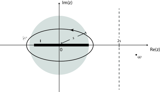
Figure 2: The imaginary part of $\omega$ should be so small that $\lvert\textup{Im}\omega\rvert=\eta<\pi/\beta$. The path $\mathscr{C}$ should enclose $\mathbf{I}$ and satisfy that $z\pm\omega\notin\mathbf{I}$. Such a $\mathscr{C}$ exists if $\omega_{0}$ lies outside the interval defined in (2.1), that is, if $\lvert\omega_{0}\rvert$ is strictly larger than two times $s$, the spectral radius of $\mathrm{\mathbf{H}}_{0}$.

As a preliminary result, we shall see that $\sigma_{21}$ can be put in the form:

$$\sigma_{21}(b,N)=-\frac{\eta}{(\eta^{2}+\omega_{0}^{2})\lvert\Lambda_{N}\rvert}\operatorname{Tr}\left\{i[\mathrm{\mathbf{j}}_{2,\textup{b},\textup{N}},\mathrm{\mathbf{X}}_{1,\textup{N}}]f_{\textup{FD}}(\mathrm{\mathbf{H}}_{\textup{N},\textup{b}})\right\}$$ (2.2)

$$+\textup{Re}\frac{1}{2\pi\omega\lvert\Lambda_{N}\rvert}\oint_{\mathscr{C}}\textup{d}z\;f_{\textup{FD}}(z)\left(\operatorname{Tr}\left\{\left(\mathrm{\mathbf{H}}_{\textup{N},\textup{b}}-z+\omega\right)^{-1}\mathrm{\mathbf{j}}_{1,\textup{b},\textup{N}}(\mathrm{\mathbf{H}}_{\textup{N},\textup{b}}-z)^{-1}\mathrm{\mathbf{j}}_{2,\textup{b},\textup{N}}\right\}+[z\to z+\omega]\right),$$

where $[z\rightarrow z+\omega]$ denotes a trace like the preceding one, just with $z$ substituted by $z+\omega$. For $z\in\rho(\mathrm{\mathbf{H}}_{b})$ define the operators on $\ell^{2}(\Lambda)$:

$$\mathrm{\mathbf{D}}_{\textup{b}}(z):=\left(\mathrm{\mathbf{H}}_{\textup{b}}-z+\omega\right)^{-1}\mathrm{\mathbf{j}}_{1,\textup{b}}(\mathrm{\mathbf{H}}_{\textup{b}}-z)^{-1}\mathrm{\mathbf{j}}_{2,\textup{b}}$$ (2.3)

where $\mathrm{\mathbf{j}}_{\nu,\textup{b}}:=i[\mathrm{\mathbf{H}}_{\textup{b}},\mathrm{\mathbf{X}}_{\nu}],\,\nu=1,2.$ We are now ready to state the main result of this paper.

Theorem 2.1.

Assume that the real part of the frequency $\omega_{0}$ is large enough. Then the following statements hold true:

(i). Assume that $\mathscr{C}_{0}$ contains the spectrum of $\mathrm{\mathbf{H}}_{\textup{b}}$, while $\mathscr{C}_{0}\pm\omega_{0}$ does not. Then the transverse conductivity admits both the thermodynamic and the adiabatic limit, and we have:

$$\begin{split}\sigma_{21}(b)&:=\lim_{\eta\to 0}\lim_{N\to\infty}\sigma_{21}(b,N)\\ &={\rm Re}\frac{1}{2\lvert\Omega\rvert\pi\omega_{0}}\oint_{\mathscr{C}_{0}}\textup{d}z\;f_{\textup{FD}}(z)\sum_{\underline{x}\in\Omega}\left(\mathrm{\mathbf{D}}_{\textup{b}}(\mbox{\boldmath$\underline{x}$},\mbox{\boldmath$\underline{x}$};z)+\mathrm{\mathbf{D}}_{\textup{b}}(\mbox{\boldmath$\underline{x}$},\mbox{\boldmath$\underline{x}$};z+\omega_{0})\right).\end{split}$$ (2.4)

(ii). In the standard nearest neighbour tight-binding model of graphene (see (1.7)), $\sigma_{21}^{G}(0)=0$.

(iii). The function $b\mapsto\sigma_{21}(b)$ is smooth and has an asymptotic expansion in $b$ around $0$. All the derivatives of $\sigma_{21}$ at zero can be written only in terms of the fiber operators associated to the Bloch decomposition of $\mathrm{\mathbf{H}}_{0}$. In particular, for the standard nearest neighbour tight-binding model of graphene, all even Taylor coefficients are zero:

$$\frac{\textup{d}^{n}\sigma_{21}^{G}}{\textup{d}b^{n}}(0)=0,\quad n=2p,\quad p\in\mathbb{N}.$$ (2.5)

3 Proof of Theorem 2.1(i)

3.1 Derivation of formula (2.2)

If $\mathrm{\mathbf{A}}$ is a bounded operator, then we denote its expression in the interaction picture with

$$\mathrm{\mathbf{\tilde{A}}}(t)=\exp\left(it\mathrm{\mathbf{H}}_{\textup{b},\textup{N}}\right)\,\mathrm{\mathbf{A}}\,\exp\left(-it\mathrm{\mathbf{H}}_{\textup{b},\textup{N}}\right).$$

By standard perturbation theory, we can write

$$\mbox{\boldmath{$\varrho$}}_{\textup{N},\textup{E}}(0)=f_{\textup{FD}}(\mathrm{\mathbf{H}}_{\textup{N},\textup{b}})-i\int_{-\infty}^{0}\textup{d}s\left[\tilde{\mathrm{\mathbf{V}}}_{\textup{N},\textup{E}}(s)\,,\,f_{\textup{FD}}(\mathrm{\mathbf{H}}_{\textup{N},\textup{b}})\right]+\mathcal{O}(E^{2})\,.$$

Thus in the linear response approximation we set

$$\mbox{\boldmath{$\varrho$}}_{\textup{N},\textup{E},\textup{lin}}(0)=f_{\textup{FD}}(\mathrm{\mathbf{H}}_{\textup{N},\textup{b}})-iE\int_{-\infty}^{0}\textup{d}s\,\textup{Re}\left(e^{i\omega s}\right)\left[\tilde{\mathrm{\mathbf{X}}}_{1\textup{N},\textup{E}}(s)\,,\,f_{\textup{FD}}(\mathrm{\mathbf{H}}_{\textup{N},\textup{b}})\right]\,.$$ (3.1)

The value of the current density in the y-direction in the linear response regime is given by

$$J_{2,\textup{b},\textup{N},\textup{lin}}(E,t=0)=\operatorname{Tr}\left\{\left(f_{\textup{FD}}(\mathrm{\mathbf{H}}_{\textup{N},\textup{b}})-iE\int_{-\infty}^{0}\textup{d}s\,\textup{Re}\left(e^{i\omega s}\right)\left[\tilde{\mathrm{\mathbf{X}}}_{1\textup{N},\textup{E}}(s)\,,\,f_{\textup{FD}}(\mathrm{\mathbf{H}}_{\textup{N},\textup{b}})\right]\right)\frac{\mathrm{\mathbf{j}}_{2,\textup{b},\textup{N}}}{\lvert\Lambda_{N}\rvert}\right\}\,.$$

Using the trace-cyclicity rule $\operatorname{Tr}\{[\mathrm{\mathbf{A}},\mathrm{\mathbf{B}}]\mathrm{\mathbf{C}}\}=\operatorname{Tr}\{\mathrm{\mathbf{B}}[\mathrm{\mathbf{C}},\mathrm{\mathbf{A}}]\}$, the equilibrium current $J_{2}(0)$ is shown to equal zero:

$$J_{2,\textup{b},\textup{N}}(0)=\operatorname{Tr}\{[f_{\textup{FD}}(\mathrm{\mathbf{H}}_{\textup{N},\textup{b}}),\mathrm{\mathbf{H}}_{\textup{N},\textup{b}}]\mathrm{\mathbf{X}}_{2,\textup{N}}\}=0.$$

By examining the formulae (1.15), (1.16) and (3.1) we can single out the transverse conductivity term:

$$\mbox{\boldmath{$\sigma$}}_{21,\textup{N}}(t=0)=-\frac{1}{\lvert\Lambda_{N}\rvert}\int_{-\infty}^{0}\textup{d}s\,\textup{Re}\left(e^{i\omega s}\right)\,\textup{Tr}\{i\left[\tilde{\mathrm{\mathbf{X}}}_{1,\textup{b},\textup{N}}(s)\,,\,f_{\textup{FD}}(\mathrm{\mathbf{H}}_{\textup{N},\textup{b}})\right]\mathrm{\mathbf{j_{2,\textup{b},\textup{N}}}}\}.$$ (3.2)

The trace in the integrand of equation (3.2) is a real number, thus formula (3.2) can be re-expressed as

$$\mbox{\boldmath{$\sigma$}}_{21,\textup{N}}(t=0)=-\frac{1}{\lvert\Lambda_{N}\rvert}\textup{Re}\int_{-\infty}^{0}\textup{d}s\,e^{i\omega s}\,\operatorname{Tr}\left\{\,i[\mathrm{\mathbf{j}}_{2,\textup{b},\textup{N}}\,,\,e^{is\mathrm{\mathbf{H}}_{\textup{N},\textup{b}}}\mathrm{\mathbf{X}}_{1,\textup{N}}e^{-is\mathrm{\mathbf{H}}_{\textup{N},\textup{b}}}]\,f_{\textup{FD}}(\mathrm{\mathbf{H}}_{\textup{N},0})\right\}.$$ (3.3)

By partial integration we re-express (3.3) as

$$\mbox{\boldmath{$\sigma$}}_{21,\textup{N}}(t=0) =-\frac{\eta}{(\eta^{2}+\omega_{0}^{2})\lvert\Lambda_{N}\rvert}\operatorname{Tr}\left\{i[\mathrm{\mathbf{j}}_{2,\textup{b},\textup{N}},\mathrm{\mathbf{X}}_{1,\textup{N}}]f_{\textup{FD}}(\mathrm{\mathbf{H}}_{\textup{N},\textup{b}})\right\}$$ (3.4)

$$\quad+\textup{Re}\frac{1}{\lvert\Lambda_{N}\rvert}\int_{-\infty}^{0}\textup{d}s\,\frac{1}{i\omega}e^{i\omega s}\frac{\textup{d}}{\textup{d}s}\left(\operatorname{Tr}\left\{i[\mathrm{\mathbf{j}}_{2,\textup{b},\textup{N}},e^{is\mathrm{\mathbf{H}}_{\textup{N},\textup{b}}}\mathrm{\mathbf{X}}_{1,\textup{N}}e^{-is\mathrm{\mathbf{H}}_{\textup{N},\textup{b}}}]f_{\textup{FD}}(\mathrm{\mathbf{H}}_{\textup{N},\textup{b}})\right\}\right).$$

We note that

$$\frac{\textup{d}}{\textup{d}t}\left(e^{it\mathrm{\mathbf{H}}_{\textup{N},\textup{b}}}\mathrm{\mathbf{X}}_{1,\textup{N}}e^{-it\mathrm{\mathbf{H}}_{\textup{N},\textup{b}}}\right)=e^{it\mathrm{\mathbf{H}}_{\textup{N},\textup{b}}}\mathrm{\mathbf{j}}_{1,\textup{b},\textup{N}}e^{-it\mathrm{\mathbf{H}}_{\textup{N},\textup{b}}},$$

by the definition of $\mathrm{\mathbf{j}}_{1,\textup{b}}$. By using the trace-cyclicity and by noticing that $f_{\textup{FD}}(\mathrm{\mathbf{H}}_{\textup{N},\textup{b}})$ and $e^{is(\omega+\mathrm{\mathbf{H}}_{\textup{N},\textup{b}})}$ commute, we have

$$\begin{split}\mbox{\boldmath{$\sigma$}}_{21,\textup{N}}(t=0)=&-\frac{\eta}{(\eta^{2}+\omega_{0}^{2})\lvert\Lambda_{N}\rvert}\operatorname{Tr}\left\{i[\mathrm{\mathbf{j}}_{2,\textup{b},\textup{N}},\mathrm{\mathbf{X}}_{1,\textup{N}}]f_{\textup{FD}}(\mathrm{\mathbf{H}}_{\textup{N},\textup{b}})\right\}\\ &+\frac{1}{\lvert\Lambda_{N}\rvert}\textup{Re}\int_{-\infty}^{0}\left(\frac{1}{\omega}\operatorname{Tr}\left\{e^{is\mathrm{\mathbf{H}}_{\textup{N},\textup{b}})}\mathrm{\mathbf{j}}_{1,\textup{b},\textup{N}}e^{-is(\mathrm{\mathbf{H}}_{\textup{N},\textup{b}}-\omega)}f_{\textup{FD}}(\mathrm{\mathbf{H}}_{\textup{N},\textup{b}})\mathrm{\mathbf{j}}_{2,\textup{b},\textup{N}}\right\}\right.\\ &\qquad\qquad\qquad\qquad\left.-\operatorname{Tr}\left\{e^{is(\omega+\mathrm{\mathbf{H}}_{\textup{N},\textup{b}})}f_{\textup{FD}}(\mathrm{\mathbf{H}}_{\textup{N},\textup{b}})\mathrm{\mathbf{j}}_{1,\textup{b},\textup{N}}e^{is\mathrm{\mathbf{H}}_{\textup{N},\textup{b}}}\mathrm{\mathbf{j}}_{2,\textup{b},\textup{N}})\right\}\right)\textup{d}s.\end{split}$$

We can use the Cauchy integral formula to express the operator $e^{is(\omega+\mathrm{\mathbf{H}}_{\textup{N},\textup{b}})}f_{\textup{FD}}(\mathrm{\mathbf{H}}_{\textup{N},\textup{b}})$ by a curve integral in the complex plane, involving the resolvent of $\mathrm{\mathbf{H}}_{\textup{N},\textup{b}}$:

$$e^{is(\omega+\mathrm{\mathbf{H}}_{\textup{N},\textup{b}})}f_{\textup{FD}}(\mathrm{\mathbf{H}}_{\textup{N},\textup{b}})=\frac{i}{2\pi}\oint_{\mathscr{C}}e^{is(z+\omega)}f_{\textup{FD}}(z)(\mathrm{\mathbf{H}}_{\textup{N},\textup{b}}-z)^{-1}dz,$$

where the path $\mathscr{C}$ encloses, but has no points in common with, the (real, bounded) spectrum, $\sigma(\mathrm{\mathbf{H}}_{\textup{b},\textup{N}})$. As mentioned, it is possible, given $\beta$, $\eta$, and $\omega_{0}$ satisfying (2.1), to choose such a curve $\mathscr{C}$ such that $\omega$ lies outside $\mathscr{C}$, and such that $f_{\textup{FD}}(z)=(e^{\beta(z-\mu)}+1)^{-1}$ has no singularities inside $\mathscr{C}$. See figure 2. This leads to

$$\begin{split}&\mbox{\boldmath{$\sigma$}}_{21,\textup{N}}(t=0)=-\frac{\eta}{(\eta^{2}+\omega_{0}^{2})\lvert\Lambda_{N}\rvert}\operatorname{Tr}\left\{i[\mathrm{\mathbf{j}}_{2,\textup{b},\textup{N}},\mathrm{\mathbf{X}}_{1,\textup{N}}]f_{\textup{FD}}(\mathrm{\mathbf{H}}_{\textup{N},\textup{b}})\right\}\\ &+\textup{Re}\int_{-\infty}^{0}\textup{d}s\,\frac{1}{\omega\lvert\Lambda_{N}\rvert}\left(\operatorname{Tr}\left\{e^{is\mathrm{\mathbf{H}}_{\textup{N},\textup{b}}}\mathrm{\mathbf{j}}_{1,\textup{b},\textup{N}}\underbrace{\left(\frac{i}{2\pi}\oint_{\mathscr{C}}\textup{d}z\;e^{-is(z-\omega)}f_{\textup{FD}}(z)(\mathrm{\mathbf{H}}_{\textup{N},\textup{b}}-z)^{-1}\right)}_{=e^{-is(\mathrm{\mathbf{H}}_{\textup{N},\textup{b}}-\omega)}f_{\textup{FD}}(\mathrm{\mathbf{H}}_{\textup{N},\textup{b}})}\mathrm{\mathbf{j}}_{2,\textup{b},\textup{N}}\right\}\right.\\ &\qquad\quad-\left.\operatorname{Tr}\left\{\underbrace{\left(\frac{i}{2\pi}\oint_{\mathscr{C}}\textup{d}z\,e^{is(z+\omega)}f_{\textup{FD}}(z)(\mathrm{\mathbf{H}}_{\textup{N},\textup{b}}-z)^{-1}\right)}_{=e^{is(\mathrm{\mathbf{H}}_{\textup{N},\textup{b}}+\omega)}f_{\textup{FD}}(\mathrm{\mathbf{H}}_{\textup{N},\textup{b}})}\mathrm{\mathbf{j}}_{1,\textup{b},\textup{N}}\,e^{-is\mathrm{\mathbf{H}}_{\textup{N},\textup{b}}}\,\mathrm{\mathbf{j}}_{2,\textup{b},\textup{N}}\right\}\right).\end{split}$$ (3.5)

The two integrals, $\oint_{\mathscr{C}}\textup{d}z\dotsi$ and $\int_{-\infty}^{0}\textup{d}s\dotsi$ in equation (3.5) are both absolutely convergent, therefore we can exchange integration order (Fubini). Furthermore, as $e^{\pm is(z\pm\omega)}$ is nothing but a complex scalar, we can freely place this factor in the operator product,

$$\begin{split}&\mbox{\boldmath{$\sigma$}}_{21,\textup{N}}(t=0)=-\frac{\eta}{(\eta^{2}+\omega_{0}^{2})\lvert\Lambda_{N}\rvert}\operatorname{Tr}\left\{i[\mathrm{\mathbf{j}}_{2,\textup{b},\textup{N}},\mathrm{\mathbf{X}}_{1,\textup{N}}]f_{\textup{FD}}(\mathrm{\mathbf{H}}_{\textup{N},\textup{b}})\right\}\\ &+\textup{Re}\oint_{\mathscr{C}}\textup{d}z\;\int_{-\infty}^{0}\textup{d}s\frac{1}{\omega\lvert\Lambda_{N}\rvert}\left(\operatorname{Tr}\left\{e^{is(\mathrm{\mathbf{H}}_{\textup{N},\textup{b}}-z+\omega)}\mathrm{\mathbf{j}}_{1,\textup{b},\textup{N}}\frac{i}{2\pi}f_{\textup{FD}}(z)(\mathrm{\mathbf{H}}_{\textup{N},\textup{b}}-z)^{-1}\mathrm{\mathbf{j}}_{2,\textup{b},\textup{N}}\right\}\right.\\ &\qquad\quad-\left.\operatorname{Tr}\left\{\frac{i}{2\pi}f_{\textup{FD}}(z)(\mathrm{\mathbf{H}}_{\textup{N},\textup{b}}-z)^{-1}\mathrm{\mathbf{j}}_{1,\textup{b},\textup{N}}e^{is(z+\omega-\mathrm{\mathbf{H}}_{\textup{N},\textup{b}})}\mathrm{\mathbf{j}}_{2,\textup{b},\textup{N}}\right\}\right).\end{split}$$

Integrating with respect to $s$ we obtain (formula (2.2)):

$$\begin{split}\mbox{\boldmath{$\sigma$}}_{21,\textup{N}}(t=0)&=-\frac{\eta}{(\eta^{2}+\omega_{0}^{2})\lvert\Lambda_{N}\rvert}\operatorname{Tr}\left\{i[\mathrm{\mathbf{j}}_{2,\textup{b},\textup{N}},\mathrm{\mathbf{X}}_{1,\textup{N}}]f_{\textup{FD}}(\mathrm{\mathbf{H}}_{\textup{N},\textup{b}})\right\}\\ &+\textup{Re}\oint_{\mathscr{C}}\textup{d}z\frac{1}{2\pi\omega\lvert\Lambda_{N}\rvert}\;f_{\textup{FD}}(z)\left(\operatorname{Tr}\left\{\left(\mathrm{\mathbf{H}}_{\textup{N},\textup{b}}-z+\omega\right)^{-1}\mathrm{\mathbf{j}}_{1,\textup{b},\textup{N}}(\mathrm{\mathbf{H}}_{\textup{N},\textup{b}}-z)^{-1}\mathrm{\mathbf{j}}_{2,\textup{b},\textup{N}}\right\}\right.\\ &\qquad\qquad+\left.\operatorname{Tr}\left\{(\mathrm{\mathbf{H}}_{\textup{N},\textup{b}}-z)^{-1}\mathrm{\mathbf{j}}_{1,\textup{b},\textup{N}}\left(\mathrm{\mathbf{H}}_{\textup{N},\textup{b}}-z-\omega\right)^{-1}\mathrm{\mathbf{j}}_{2,\textup{b},\textup{N}}\right\}\right).\end{split}$$ (3.6)

3.2 Off-diagonal localization for resolvents

In this subsection we only work with operators defined on $\ell^{2}(\Lambda)$. It should be understood that the results 3.1-3.5 also hold true, even if $\Lambda$ is replaced with $\Lambda_{N}$, uniformly in $N$.

Definition 3.1 (Schur-Holmgren bound).

For a linear operator $\mathrm{\mathbf{A}}\in B\left(\ell^{2}(\Lambda)\right)$ with a kernel $a(\mbox{\boldmath$x$},\mbox{\boldmath$x$}^{\prime})$, we define the Schur-Holmgren bound by:

$$\lVert\mathrm{\mathbf{A}}\rVert_{1}:=\max\left\{\sup_{\mbox{\boldmath$x$}\in\Lambda}\sum_{\mbox{\boldmath$x$}^{\prime}\in\Lambda}\lvert a(\mbox{\boldmath$x$},\mbox{\boldmath$x$}^{\prime})\rvert,\sup_{\mbox{\boldmath$x$}^{\prime}\in\Lambda}\sum_{\mbox{\boldmath$x$}\in\Lambda}\lvert a(\mbox{\boldmath$x$},\mbox{\boldmath$x$}^{\prime})\rvert\right\}$$ (3.7)

If an operator has $\lVert\mathrm{\mathbf{A}}\rVert_{1}<\infty$ it is said to be Schur-Holmgren bounded.

The following bound is well known, and we give it without proof:

Lemma 3.2.

Let $\mathrm{\mathbf{A}}\in B\left(\ell^{2}(\Lambda)\right)$. If $\lVert\mathrm{\mathbf{A}}\rVert_{1}<\infty$, then $\lVert\mathrm{\mathbf{A}}\rVert\leq\lVert\mathrm{\mathbf{A}}\rVert_{1}$, where $\lVert\mathrm{\mathbf{A}}\rVert$ is the usual operator norm.

Definition 3.3 (Exponentially Almost Diagonal Operator).

Let $\mathrm{\mathbf{A}}\in B\left(\ell^{2}(\Lambda)\right)$. We say that $\mathrm{\mathbf{A}}$ is exponentially almost diagonal, if there exist two constants $C_{1},C_{2}$, both strictly positive, so that the kernel of $\mathrm{\mathbf{A}}$ satisfies

$$\lvert a(\mbox{\boldmath$x$},\mbox{\boldmath$y$})\rvert\leq C_{1}e^{-C_{2}\lVert\mbox{\boldmath$x$}-\mbox{\boldmath$y$}\rVert}$$ (3.8)

for all $\mbox{\boldmath$x$},\mbox{\boldmath$y$}$ in $\Lambda$.

The proof of the next lemma is straightforward and thus omitted.

Lemma 3.4.

An exponentially almost diagonal operator is Schur-Holmgren bounded (and by lemma 3.2 bounded).

We now show a property for exponentially almost diagonal operators, which is a much simpler version of the Combes-Thomas estimate for resolvents of continuous Schrödinger operators [9, 10].

Proposition 3.5 (CT-property).

Let $z\in\rho(\mathrm{\mathbf{A}})$ where $\mathrm{\mathbf{A}}\in B\left(\ell^{2}(\Lambda)\right)$ is a self-adjoint exponentially almost diagonal operator. Let constants $C_{1}$ and $C_{2}$ be defined as in definition (3.8).

Then the resolvent $(\mathrm{\mathbf{A}}-z)^{-1}$ is also exponentially almost diagonal. That is, there exists two positive constants $C_{3}$ and $C_{4}$ such that the kernel of $(\mathrm{\mathbf{A}}-z)^{-1}$ fulfils

$$\lvert(\mathrm{\mathbf{A}}-z)^{-1}(\mbox{\boldmath$x$},\mbox{\boldmath$y$})\rvert\leq C_{3}e^{-C_{4}\lVert\mbox{\boldmath$x$}-\mbox{\boldmath$y$}\rVert}.$$

Consider the situation where $z$ is restricted to a closed subset $\mathscr{C}\subset\rho(\mathrm{\mathbf{A}})$. Then $C_{3}$ and $C_{4}$ can be chosen uniformly in $\textup{dist}(\mathscr{C},\sigma(\mathrm{\mathbf{A}})\,)$.

Proof.

We only sketch the main ideas, see [11] for a related result. For $\alpha>0$, and a fixed lattice point $\mbox{\boldmath$x$}_{0}\in\Lambda$, define the operator $\mathrm{\mathbf{A}}_{\alpha}:\ell^{2}(\Lambda)\to\ell^{2}(\Lambda)$ by

$$\mathrm{\mathbf{A}}_{\alpha}:=e^{\alpha\lVert\cdot\,-\mbox{\boldmath$x$}_{0}\rVert}\mathrm{\mathbf{A}}e^{-\alpha\lVert\cdot\,-\mbox{\boldmath$x$}_{0}\rVert}.$$

It can be shown that

$$\lVert\mathrm{\mathbf{A}}-\mathrm{\mathbf{A}}_{\alpha}\rVert_{1}\,\autorightarrow{\alpha\to 0}{}\,0.$$ (3.9)

By the identity

$$(\mathrm{\mathbf{A}}_{\alpha}-z)=(\mathrm{\mathbf{I}}-(\mathrm{\mathbf{A}}-\mathrm{\mathbf{A}}_{\alpha})(\mathrm{\mathbf{A}}-z)^{-1})(\mathrm{\mathbf{A}}-z),$$

the operator $(\mathrm{\mathbf{A}}_{\alpha}-z)$ is invertible for $\alpha$ small enough depending on $z$. We can write the equality

$$e^{-\alpha\lVert\cdot\,-\mbox{\boldmath$x$}_{0}\rVert}(\mathrm{\mathbf{A}}_{\alpha}-z)=(\mathrm{\mathbf{A}}-z)e^{-\alpha\lVert\cdot\,-\mbox{\boldmath$x$}_{0}\rVert},$$

which implies that

$$(\mathrm{\mathbf{A}}-z)^{-1}e^{-\alpha\lVert\cdot\,-\mbox{\boldmath$x$}_{0}\rVert}=e^{-\alpha\lVert\cdot\,-\mbox{\boldmath$x$}_{0}\rVert}(\mathrm{\mathbf{A}}_{\alpha}-z)^{-1},$$

and which gives

$$e^{\alpha\lVert\cdot\,-\mbox{\boldmath$x$}_{0}\rVert}(\mathrm{\mathbf{A}}-z)^{-1}e^{-\alpha\lVert\cdot\,-\mbox{\boldmath$x$}_{0}\rVert}=(\mathrm{\mathbf{A}}_{\alpha}-z)^{-1}.$$

If we apply both sides on the basis element $\delta_{\mbox{\boldmath$x$}_{0}}$ and then take the scalar product with some $\delta_{\mbox{\boldmath$x$}}$ we get:

$$\langle\delta_{\mbox{\boldmath$x$}},e^{\alpha\lVert\cdot\,-\mbox{\boldmath$x$}_{0}\rVert}(\mathrm{\mathbf{A}}-z)^{-1}e^{-\alpha\lVert\cdot\,-\mbox{\boldmath$x$}_{0}\rVert}\delta_{\mbox{\boldmath$x$}_{0}}\rangle=e^{\alpha\lVert\mbox{\boldmath$x$}-\mbox{\boldmath$x$}_{0}\rVert}(\mathrm{\mathbf{A}}-z)^{-1}(\mbox{\boldmath$x$},\mbox{\boldmath$x$}_{0})=\langle\delta_{\mbox{\boldmath$x$}},(\mathrm{\mathbf{A}}_{\alpha}-z)^{-1}\delta_{\mbox{\boldmath$x$}_{0}}\rangle,$$

which means that

$$e^{\alpha\lVert\mbox{\boldmath$x$}-\mbox{\boldmath$x$}_{0}\rVert}\left|(\mathrm{\mathbf{A}}-z)^{-1}(\mbox{\boldmath$x$},\mbox{\boldmath$x$}_{0})\right|\leq\left\|(\mathrm{\mathbf{A}}_{\alpha}-z)^{-1}\right\|.$$

This formula can be used in order to get the desired estimate for the integral kernel. We do not give further details. ∎

The last preparatory results are concerned with the magnetic translations. We define the magnetic translation operator as the operator that transforms $\mbox{\boldmath$\psi$}\in\ell^{2}(\Lambda)$ according to the rule:

$$\left(\mathrm{\mathbf{\mathcal{T}}}_{\textup{b},\gamma}\mbox{\boldmath$\psi$}\right)(\mbox{\boldmath$x$}):=e^{ib\varphi(\mbox{\boldmath$x$},\mbox{\boldmath$\gamma$})}\psi(\mbox{\boldmath$x$}-\mbox{\boldmath$\gamma$}),\qquad\textup{for all }\mbox{\boldmath$\gamma$}\in\Gamma,\mbox{\boldmath$x$}\in\Lambda.$$

The magnetic translations have certain properties which we list here without proof. The inverse of the magnetic translation operator obeys

$$\mathrm{\mathbf{\mathcal{T}}}_{\textup{b},\gamma}^{-1}=\mathrm{\mathbf{\mathcal{T}}}_{\textup{b},-\gamma}.$$

The Hamilton operator $\mathrm{\mathbf{H}}_{\textup{b}}$ commutes with $\mathrm{\mathbf{\mathcal{T}}}_{\textup{b},\gamma}$ for all $\gamma\in\Gamma$. The same property is true for the current operator whose integral kernel is

$$\mathrm{\mathbf{j}}_{\nu,\textup{b}}(\mbox{\boldmath$x$},\mbox{\boldmath$y$})=ih_{\textup{b}}(\mbox{\boldmath$x$},\mbox{\boldmath$y$})(y_{\nu}-x_{\nu})=e^{ib\varphi(\mbox{\boldmath$x$},\mbox{\boldmath$y$})}\mathrm{\mathbf{j}}_{\nu,0}(\mbox{\boldmath$x$},\mbox{\boldmath$y$}),\quad\nu\in\{1,2\}.$$

3.3 Proof of the thermodynamic and adiabatic limits

Let us briefly discuss the first term appearing in (2.2), that is

$$\frac{\eta}{(\eta^{2}+\omega_{0}^{2})\lvert\Lambda_{N}\rvert}\operatorname{Tr}\left\{i[\mathrm{\mathbf{j}}_{2,\textup{b},\textup{N}},\mathrm{\mathbf{X}}_{1,\textup{N}}]f_{\textup{FD}}(\mathrm{\mathbf{H}}_{\textup{N},\textup{b}})\right\}.$$

We have the identity:

$$i[\mathrm{\mathbf{j}}_{2,\textup{b},\textup{N}},\mathrm{\mathbf{X}}_{1,\textup{N}}](\mbox{\boldmath$x$},\mbox{\boldmath$y$})=i\chi_{\textup{N}}(\mbox{\boldmath$x$})h_{b}(\mbox{\boldmath$x$},\mbox{\boldmath$y$})(y_{2}-x_{2})(y_{1}-x_{1})\chi_{\textup{N}}(\mbox{\boldmath$y$}),$$

which defines a bounded operator due to the localization properties of $h_{0}$. This means in particular that $\operatorname{Tr}\left\{i[\mathrm{\mathbf{j}}_{2,\textup{b},\textup{N}},\mathrm{\mathbf{X}}_{1,\textup{N}}]f_{\textup{FD}}(\mathrm{\mathbf{H}}_{\textup{N},\textup{b}})\right\})/\lvert\Lambda_{N}\rvert$ is bounded in $N$ uniformly in $\eta$, thus after the adiabatic limit this term will disappear anyway. That is why we only treat in detail the second term of (2.2).

First, we need to introduce some notation. Let $0<\epsilon<1$. We divide our finite box, $\Lambda_{N}$, into an edge region $\tilde{\tilde{\Lambda}}_{N}$ of width $[N^{\epsilon}]$ unit cells, and a remaining core part, $\tilde{\Lambda}_{N}$, see figure 3. We have that $\tilde{\tilde{\Lambda}}_{N}=\Lambda_{N}\setminus\tilde{\Lambda}_{N}$. For practical reasons we work with $N^{\epsilon}$ instead of its integer part.

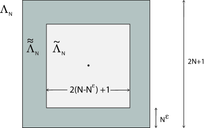
Figure 3: $\Lambda_{N}$ is split into a core part, $\tilde{\Lambda}_{N}$, $2(N-N^{\epsilon})+1$ unit cells wide and an edge region $\tilde{\tilde{\Lambda}}_{N}$ of width $N^{\epsilon}$ unit cells. $0<\epsilon<1$

The number of unit cells in $\tilde{\tilde{\Lambda}}_{N}$ is $N^{1+\epsilon}$, which means $\frac{\lvert\tilde{\tilde{\Lambda}}_{N}\rvert}{N^{2}}\to 0$ as $N$ tends to infinity. As a consequence, the number unit cells in $\tilde{\Lambda}_{N}$ behaves like $4N^{2}$ for large $N$.

3.3.1 Geometric perturbation theory

To simplify notation, we introduce a shorthand for the characteristic functions $\tilde{\chi}_{\textup{N}}=\chi_{\tilde{\Lambda}_{N}}$, $\tilde{\tilde{\chi}}_{\textup{N}}~{}=~{}\chi_{\tilde{\tilde{\Lambda}}_{N}}$. We now introduce an auxilliary operator by:

$$\mathrm{\mathbf{A}}_{\textup{b},\textup{N}}(z)=\tilde{\chi}_{\textup{N}}\left(\mathrm{\mathbf{H}}_{\textup{b}}-z\right)^{-1}\tilde{\chi}_{\textup{N}}+\tilde{\tilde{\chi}}_{\textup{N}}\left(\mathrm{\mathbf{H}}_{\textup{b},\textup{N}}-z\right)^{-1}\tilde{\tilde{\chi}}_{\textup{N}},\quad z\in\mathscr{C}.$$

If we multiply $\mathrm{\mathbf{A}}_{\textup{b},\textup{N}}(z)$ on the left by $\left(\mathrm{\mathbf{H}}_{\textup{b},\textup{N}}-z\right)$, we have

$$\left(\mathrm{\mathbf{H}}_{\textup{b},\textup{N}}-z\right)\mathrm{\mathbf{A}}_{\textup{b},\textup{N}}(z) =\left(\mathrm{\mathbf{H}}_{\textup{b},\textup{N}}-z\right)\tilde{\chi}_{\textup{N}}\left(\mathrm{\mathbf{H}}_{\textup{b}}-z\right)^{-1}\tilde{\chi}_{\textup{N}}+\left(\mathrm{\mathbf{H}}_{\textup{b},\textup{N}}-z\right)\tilde{\tilde{\chi}}_{\textup{N}}\left(\mathrm{\mathbf{H}}_{\textup{b},\textup{N}}-z\right)^{-1}\tilde{\tilde{\chi}}_{\textup{N}}.$$ (3.10)

Note that for large enough $N$, the distance between $\tilde{\Lambda}_{N}$ and $\Lambda\setminus\Lambda_{N}$ becomes larger than the interaction range of $\mathrm{\mathbf{H}}_{\textup{b},\textup{N}}$. This implies that $\left(\mathrm{\mathbf{H}}_{\textup{b},\textup{N}}-z\right)\tilde{\chi}_{\textup{N}}=\left(\mathrm{\mathbf{H}}_{\textup{b}}-z\right)\tilde{\chi}_{\textup{N}}$. Therefore, if we use this in the first term of formula (3.10), and using that $\tilde{\chi}_{\textup{N}}+\tilde{\tilde{\chi}}_{\textup{N}}=\chi_{\textup{N}}$, (3.10) becomes:

$$\left(\mathrm{\mathbf{H}}_{\textup{b},\textup{N}}-z\right)\mathrm{\mathbf{A}}_{\textup{b},\textup{N}}(z) =\chi_{\textup{N}}+[\mathrm{\mathbf{H}}_{\textup{b}},\tilde{\chi}_{\textup{N}}]\left(\mathrm{\mathbf{H}}_{\textup{b}}-z\right)^{-1}\tilde{\chi}_{\textup{N}}+[\mathrm{\mathbf{H}}_{\textup{b},\textup{N}},\tilde{\tilde{\chi}}_{\textup{N}}]\left(\mathrm{\mathbf{H}}_{\textup{b},\textup{N}}-z\right)^{-1}\tilde{\tilde{\chi}}_{\textup{N}},$$

which is equivalent with:

$$\left(\mathrm{\mathbf{H}}_{\textup{b},\textup{N}}-z\right)^{-1} =\mathrm{\mathbf{A}}_{\textup{b},\textup{N}}(z)-\left(\mathrm{\mathbf{H}}_{\textup{b},\textup{N}}-z\right)^{-1}\mathrm{\mathbf{B}}_{\textup{b},\textup{N}}(z),$$ (3.11)

where:

$$\mathrm{\mathbf{B}}_{\textup{b},\textup{N}}(z)=[\mathrm{\mathbf{H}}_{\textup{b}},\tilde{\chi}_{\textup{N}}]\left(\mathrm{\mathbf{H}}_{\textup{b}}-z\right)^{-1}\tilde{\chi}_{\textup{N}}+[\mathrm{\mathbf{H}}_{\textup{b},\textup{N}},\tilde{\tilde{\chi}}_{\textup{N}}]\left(\mathrm{\mathbf{H}}_{\textup{b},\textup{N}}-z\right)^{-1}\tilde{\tilde{\chi}}_{\textup{N}}.$$

We insert (3.11) in formula (3.6) obtaining several terms. We claim that only the following term contributes in the large $N$ limit:

$$\textup{Re}\frac{1}{2\pi\omega\lvert\Lambda_{N}\rvert}\oint_{\mathscr{C}}\textup{d}z\;f_{\textup{FD}}(z)\left(\operatorname{Tr}\left\{\tilde{\chi}_{\textup{N}}\left(\mathrm{\mathbf{H}}_{\textup{b}}-z+\omega\right)^{-1}\tilde{\chi}_{\textup{N}}\mathrm{\mathbf{j}}_{1,\textup{N}}\tilde{\chi}_{\textup{N}}(\mathrm{\mathbf{H}}_{\textup{b}}-z)^{-1}\tilde{\chi}_{\textup{N}}\mathrm{\mathbf{j}}_{2,\textup{N}}\right\}+[z\rightarrow z+\omega]\right).$$ (3.12)

The other terms in the expansion of formula (3.6) have factors of type $\tilde{\tilde{\chi}}_{\textup{N}}\left(\mathrm{\mathbf{H}}_{\textup{b},\textup{N}}-z\right)^{-1}$, $[\mathrm{\mathbf{H}}_{\textup{b}},\tilde{\chi}_{\textup{N}}]$ or $[\mathrm{\mathbf{H}}_{\textup{b},\textup{N}},\tilde{\tilde{\chi}}_{\textup{N}}]$. In the large $N$ limit terms having these factors vanish, which we explain in the following.

To begin with, let us choose one such term which up to trace cyclicity can be written as

$$\frac{1}{\lvert\Lambda_{N}\rvert}\operatorname{Tr}\left\{[\mathrm{\mathbf{H}}_{\textup{b}},\tilde{\chi}_{\textup{N}}]\mathrm{\mathbf{Q}}_{b,\textup{N}}(z)\right\},\quad z\in\mathscr{C},$$

where $\mathrm{\mathbf{Q}}_{b,\textup{N}}(z)$ is bounded uniformly in $b$, $N$, and $z$. Because the operator $\mathrm{\mathbf{H}}_{\textup{b}}$ is short-range, we can find a projection $\mathrm{\mathbf{P}}_{\textup{N}}$ whose corresponding subspace has a dimension $D\sim N^{1+\epsilon}$, such that $\mathrm{\mathbf{P}}_{\textup{N}}[\mathrm{\mathbf{H}}_{\textup{b}},\tilde{\chi}_{\textup{N}}]=[\mathrm{\mathbf{H}}_{\textup{b}},\tilde{\chi}_{\textup{N}}]$. We then use the inequality

$$\lvert\operatorname{Tr}\left\{[\mathrm{\mathbf{H}}_{\textup{b}},\tilde{\chi}_{\textup{N}}]\mathrm{\mathbf{Q}}_{b,\textup{N}}(z)\right\}\rvert\leq C\operatorname{Tr}\left\{\mathrm{\mathbf{P}}_{\textup{N}}\right\}\sim N^{1+\epsilon},$$

where $C$ is a constant uniform in $b$, $N$, and $z$. Thus by dividing by $N^{2}$, it will converge to zero. The same type of proof applies for all other terms containing $\tilde{\tilde{\chi}}_{\textup{N}}$ which can already play the role of $\mathrm{\mathbf{P}}_{\textup{N}}$.

We now consider the term given by formula (3.12), and we want to show that we can replace $\tilde{\chi}_{\textup{N}}\mathrm{\mathbf{j}}_{1,\textup{N}}\tilde{\chi}_{\textup{N}}$ with $\mathrm{\mathbf{j}}_{1}$. If we write

$$\tilde{\chi}_{\textup{N}}=\mathrm{\mathbf{I}}-(\mathrm{\mathbf{I}}-\tilde{\chi}_{\textup{N}}),$$

then the trace in (3.12) can be written as:

$$\operatorname{Tr}\left\{\tilde{\chi}_{\textup{N}}\left(\mathrm{\mathbf{H}}_{\textup{b}}-z+\omega\right)^{-1}\left(\mathrm{\mathbf{I}}-(\mathrm{\mathbf{I}}-\tilde{\chi}_{\textup{N}})\right)\mathrm{\mathbf{j}}_{1}\left(\mathrm{\mathbf{I}}-(\mathrm{\mathbf{I}}-\tilde{\chi}_{\textup{N}})\right)(\mathrm{\mathbf{H}}_{\textup{b}}-z)^{-1}\tilde{\chi}_{\textup{N}}\mathrm{\mathbf{j}}_{2}\tilde{\chi}_{\textup{N}}\right\}+[z\rightarrow z+\omega].$$ (3.13)

This trace, and thereby formula (3.12), can now be expanded into several terms, all but one containing at least one factor of the type $(\mathrm{\mathbf{I}}-\tilde{\chi}_{\textup{N}})$. The terms containing $(\mathrm{\mathbf{I}}-\tilde{\chi}_{\textup{N}})=(\mathrm{\mathbf{I}}-\chi_{\textup{N}}+\tilde{\tilde{\chi}}_{\textup{N}})$ as a factor can be written (up to trace cyclicity) in the form

$$\textup{Re}\frac{1}{2\pi\omega\lvert\Lambda_{N}\rvert}\oint_{\mathscr{C}}\textup{d}z\;f_{\textup{FD}}(z)\operatorname{Tr}\left\{(\mathrm{\mathbf{I}}-\chi_{\textup{N}})\mathrm{\mathbf{E}}_{\textup{b}}(z)\tilde{\chi}_{\textup{N}}\mathrm{\mathbf{Q}}_{b,\textup{N}}^{(1)}(z)+\tilde{\tilde{\chi}}_{\textup{N}}\mathrm{\mathbf{Q}}_{b,\textup{N}}^{(2)}(z)\right\},$$ (3.14)

where $\mathrm{\mathbf{E}}_{\textup{b}}(z)$ is an exponentially almost diagonal operator and $\mathrm{\mathbf{Q}}^{(1)}_{b,\textup{N}}(z)$ and $\mathrm{\mathbf{Q}}^{(2)}_{b,\textup{N}}(z)$ are bounded, uniformly in $b$, $N$ and $z$. The term $\tilde{\tilde{\chi}}_{\textup{N}}\mathrm{\mathbf{Q}}^{(2)}_{b,\textup{N}}(z)$ vanishes as $N$ tends to infinity by previous arguments. Now consider the term containing $(\mathrm{\mathbf{I}}-\chi_{\textup{N}})\mathrm{\mathbf{E}}_{\textup{b}}(z)\tilde{\chi}_{\textup{N}}$. The kernel $k(\mbox{\boldmath$x$},\mbox{\boldmath$y$})$ of this operator is zero unless $\lVert\mbox{\boldmath$x$}-\mbox{\boldmath$y$}\rVert>N^{\epsilon}$, see figure 3. One can easily show that the trace-norm of this operator is bounded from above by $C_{1}e^{-C_{2}N^{\epsilon}}$, for some positive constants $C_{1}$ and $C_{2}$. Thus this term will not give a contribution to the thermodynamic limit. The only remaining contribution from formula (3.12) is

$$\begin{split}&\textup{Re}\frac{1}{2\pi\omega\lvert\Lambda_{N}\rvert}\oint_{\mathscr{C}}\textup{d}z\;f_{\textup{FD}}(z)\left(\operatorname{Tr}\left\{\tilde{\chi}_{\textup{N}}\left(\mathrm{\mathbf{H}}_{\textup{b}}-z+\omega\right)^{-1}\mathrm{\mathbf{j}}_{1,\textup{b}}(\mathrm{\mathbf{H}}_{\textup{b}}-z)^{-1}\mathrm{\mathbf{j}}_{2,\textup{b}}\tilde{\chi}_{\textup{N}}\right\}\right.\\ &\qquad\qquad+\left.\operatorname{Tr}\left\{\tilde{\chi}_{\textup{N}}(\mathrm{\mathbf{H}}_{\textup{b}}-z)^{-1}\mathrm{\mathbf{j}}_{1,\textup{b}}\left(\mathrm{\mathbf{H}}_{\textup{b}}-z-\omega\right)^{-1}\mathrm{\mathbf{j}}_{2,\textup{b}}\tilde{\chi}_{\textup{N}}\right\}\right).\end{split}$$ (3.15)

Using the operators defined in (2.3), the previous formula can be re-written as

$$\textup{Re}\frac{1}{2\pi\omega\lvert\Lambda_{N}\rvert}\oint_{\mathscr{C}}\textup{d}z\;f_{\textup{FD}}(z)\left(\sum_{\mbox{\boldmath$x$}\in\tilde{\Lambda}_{N}}\mathrm{\mathbf{D}}_{\textup{b}}(\mbox{\boldmath$x$},\mbox{\boldmath$x$};z)+\mathrm{\mathbf{D}}_{\textup{b}}(\mbox{\boldmath$x$},\mbox{\boldmath$x$};z+\omega)\right).$$ (3.16)

$\mathrm{\mathbf{D}}_{\textup{b}}(z)$ is a product of operators which commute with magnetic translations. This implies that the diagonal elements of its integral kernel define a periodic function, that is for any $\mbox{\boldmath$\underline{x}$}\in\Omega$ and $\mbox{\boldmath$\gamma$}\in\Gamma$, we have that

$$\mathrm{\mathbf{D}}_{\textup{b},\pm}(\mbox{\boldmath$\underline{x}$}+\mbox{\boldmath$\gamma$},\mbox{\boldmath$\underline{x}$}+\mbox{\boldmath$\gamma$};z)=\mathrm{\mathbf{D}}_{\textup{b},\pm}(\mbox{\boldmath$\underline{x}$},\mbox{\boldmath$\underline{x}$};z).$$

Now the proof of (2.4) is straightforward and the thermodynamic and adiabatic limits are proved.

4 Proof of Theorem 2.1(ii)

Here we need to compute the transverse conductivity component at $b=0$ and prove that it gives zero if we work with the operator (1.7). We will do this computation for a general nearest neighbor model, and use the graphene model only at the end.

4.1 The Bloch-Floquet representation

In order to fix notation, we define $\mathscr{H}_{\textup{F}}:=\int_{\Omega^{*}}^{\oplus}\textup{d}^{2}k\,\,\ell^{2}(\Omega)$. The Floquet unitary [10] $\mathrm{\mathbf{U}}:\ell^{2}(\Lambda)\to\mathscr{H}_{\textup{F}}$ takes vectors $\psi$ from $\ell^{2}(\Lambda)$ into $\mathscr{H}_{\textup{F}}$, and is given by the well-known formula

$$(\mathrm{\mathbf{U}}\mbox{\boldmath$\psi$})(\mbox{\boldmath$k$},\mbox{\boldmath$\underline{x}$})=\frac{1}{\sqrt{\lvert\Omega^{*}\rvert}}\sum_{\gamma\in\Gamma}\exp(-i\mbox{\boldmath$k$}\cdot\mbox{\boldmath$\gamma$})\psi(\mbox{\boldmath$\underline{x}$}+\mbox{\boldmath$\gamma$}),\quad\mbox{\boldmath$k$}\in\Omega^{*},\mbox{\boldmath$\underline{x}$}\in\Omega.$$ (4.1)

If $\mathrm{\mathbf{A}}$ is any bounded self-adjoint operator commuting with the translations induced by the Bravais lattice $\Gamma$, we have that $\mathrm{\mathbf{U}}\mathrm{\mathbf{A}}\mathrm{\mathbf{U}}^{*}:\mathscr{H}_{\textup{F}}\to\mathscr{H}_{\textup{F}}$ is given by

$$\mathrm{\mathbf{U}}\mathrm{\mathbf{A}}\mathrm{\mathbf{U}}^{*}=\int_{\Omega^{*}}^{\oplus}a_{\textup{F}}(\mbox{\boldmath$k$})\,\textup{d}\mbox{\boldmath$k$},$$

where the fibers have the kernels (we assume that $a(\mbox{\boldmath$\underline{x}$}+\mbox{\boldmath$\gamma$},\mbox{\boldmath$\underline{y}$})$ has a sufficiently fast decay with $\gamma$):

$$a_{\textup{F}}(\mbox{\boldmath$\underline{x}$},\mbox{\boldmath$\underline{y}$};\mbox{\boldmath$k$})=\sum_{\gamma\in\Gamma}e^{-i\mbox{\boldmath$k$}\cdot\mbox{\boldmath$\gamma$}}a(\mbox{\boldmath$\underline{x}$}+\mbox{\boldmath$\gamma$},\mbox{\boldmath$\underline{y}$}).$$ (4.2)

We denoted the number of sites of $\Omega$ with $\nu_{\Omega}$. For each $\mbox{\boldmath$k$}\in\Omega^{*}$, $a_{\textup{F}}(\mbox{\boldmath$k$})$ is self-adjoint and has $\nu_{\Omega}$ real eigenvalues. Each matrix-component of $a_{\textup{F}}(\mbox{\boldmath$k$})$, viewed as a function of $k$, extends to a $\Gamma^{*}$-periodic $C^{\infty}(\mathbb{R}^{2})$ function. We order these eigenvalues in increasing order:

$$\epsilon_{1}(\mbox{\boldmath$k$})\leq\epsilon_{2}(\mbox{\boldmath$k$})\leq\dots\leq\epsilon_{\nu_{\Omega}}(\mbox{\boldmath$k$}).$$

In order to have periodic boundary conditions in the fibers, we modify (4.1) with a complex phase and define:

$$\mathrm{\mathbf{U}}_{\textup{F}}:\ell^{2}(\Lambda)\to\mathscr{H}_{\textup{F}},\qquad\left(\mathrm{\mathbf{U}}_{\textup{F}}\mbox{\boldmath$\psi$}\right)(\mbox{\boldmath$k$},\mbox{\boldmath$\underline{x}$})=\sum_{\gamma\in\Gamma}e^{-i\mbox{\boldmath$k$}\cdot(\mbox{\boldmath$\underline{x}$}+\mbox{\boldmath$\gamma$})}\psi(\mbox{\boldmath$\underline{x}$}+\mbox{\boldmath$\gamma$}),~{}$$ (4.3)

for all $\mbox{\boldmath$\psi$}\in\ell^{2}_{c}(\Lambda)$. Accordingly $\mathrm{\mathbf{U}}_{\textup{F}}\mathrm{\mathbf{H}}_{0}\mathrm{\mathbf{U}}^{*}_{\textup{F}}:\mathscr{H}_{\textup{F}}\to\mathscr{H}_{\textup{F}}$ has the fibers

$$\tilde{h}_{0}(\underline{x},\underline{y};\mbox{\boldmath$k$})=\sum_{\mbox{\boldmath$\gamma$}\in\Gamma}h_{0}(\underline{x}+\mbox{\boldmath$\gamma$},\underline{y})e^{-i\mbox{\boldmath$k$}\cdot(\underline{x}+\mbox{\boldmath$\gamma$}-\underline{y})}.$$

If we differentiate the fiber with respect to the first component of $k$, we have

$$\frac{\partial}{\partial k_{1}}\tilde{h}_{0}(\mbox{\boldmath$\underline{x}$},\mbox{\boldmath$\underline{y}$};\mbox{\boldmath$k$})=-\sum_{\gamma\in\Gamma}e^{-i\mbox{\boldmath$k$}\cdot(\mbox{\boldmath$\underline{x}$}+\mbox{\boldmath$\gamma$}-\mbox{\boldmath$\underline{y}$})}\;i(\underline{x}_{1}+\gamma_{1}-\underline{y}_{1})h(\mbox{\boldmath$\underline{x}$}+\mbox{\boldmath$\gamma$},\mbox{\boldmath$\underline{y}$}).$$ (4.4)

The expression (4.4) is nothing but the fiber of the transformed current operator $\mathrm{\mathbf{U}}_{\textup{F}}\,(i[\mathrm{\mathbf{H}},\mathrm{\mathbf{X}}_{1}])\,\mathrm{\mathbf{U}}^{*}_{\textup{F}}$.

In particular, for the graphene-Hamiltonian (1.7) we have $\nu_{\Omega}=4$, with the numbering of the basis positions given in (1.4):

$$\tilde{h}_{0}^{G}(\mbox{\boldmath$k$})=\left[\begin{array}[]{cccc}0&e^{ik_{1}a}&0&2e^{-\frac{ik_{1}a}{2}}\cos\left(\frac{\sqrt{3}k_{2}a}{2}\right)\\ \vskip 6.0pt plus 2.0pt minus 2.0pt\cr{e^{-ik_{1}a}}&0&2e^{\frac{ik_{1}a}{2}}\cos\left(\frac{\sqrt{3}k_{2}a}{2}\right)&0\\ \vskip 6.0pt plus 2.0pt minus 2.0pt\cr 0&2e^{-\frac{ik_{1}a}{2}}\cos\left(\frac{\sqrt{3}k_{2}a}{2}\right)&0&e^{ik_{1}a}\\ \vskip 6.0pt plus 2.0pt minus 2.0pt\cr 2e^{\frac{ik_{1}a}{2}}\cos\left(\frac{\sqrt{3}k_{2}a}{2}\right)&0&e^{-ik_{1}a}&0\end{array}\right].$$

We see that all matrix elements are even in $k_{2}$. The bandstructure is given by the eigenvalues of $\tilde{h}_{0}^{G}(\mbox{\boldmath$k$})$ which are shown in figure 4.

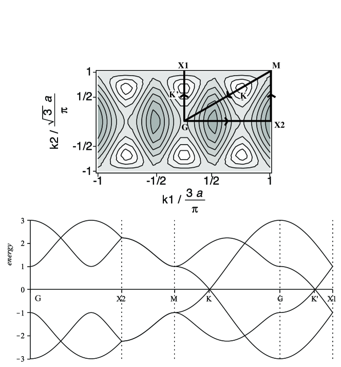
Figure 4: The bandstructure of the standard nearest neighbour tight-binding model of Graphene. Top: a figure of the first Brillouin zone, with the level-curves of $e_{3}(k_{1},k_{2})$ plotted, also showing some points of interest: $G$ (origin) $X1,X2,M,K$ and $K^{\prime}$. $K$ and $K^{\prime}$ are the two “Dirac points”. Bottom: the plot of the Bloch energies along the path indicated in the top figure.

Now if we have two operators $\mathrm{\mathbf{A}},\mathrm{\mathbf{B}}\in B(\ell^{2}(\Lambda))$, both $\Gamma$-periodic, then it holds that:

$$(\mathrm{\mathbf{A}}\mathrm{\mathbf{B}})(\mbox{\boldmath$\underline{x}$},\mbox{\boldmath$\underline{y}$};\mbox{\boldmath$k$})=\sum_{\mbox{\boldmath$\underline{x}$}^{\prime}\in\Omega}a(\mbox{\boldmath$\underline{x}$},\mbox{\boldmath$\underline{x}$}^{\prime};k)b(\mbox{\boldmath$\underline{x}$}^{\prime},\mbox{\boldmath$\underline{y}$};k).$$ (4.5)

When $b$ is equal to zero, formula (2.4) becomes:

$$\sigma_{21}(0) =\frac{1}{2\lvert\Omega\rvert\pi\omega_{0}}\textup{Re}\oint_{\mathscr{C}}\textup{d}z\;f_{\textup{FD}}(z)\sum_{\underline{x}\in\Omega}\left(\left[(\mathrm{\mathbf{H}}_{0}-z+\omega_{0})^{-1}\mathrm{\mathbf{j}}_{1,0}(\mathrm{\mathbf{H}}_{0}-z)^{-1}\mathrm{\mathbf{j}}_{2,0}\right](\mbox{\boldmath$\underline{x}$},\mbox{\boldmath$\underline{x}$})+[z\rightarrow z+\omega_{0}]\right).$$

In order to shorter notation, we denote by $r_{0}(z,\mbox{\boldmath$k$})=(\tilde{h}_{0}(\mbox{\boldmath$k$})-z)^{-1}$ the fiber of the resolvent $(\mathrm{\mathbf{H}}_{0}-z)^{-1}$. Using (4.5) we can write

$$\begin{split}&\sigma_{21}(0)=\frac{1}{2\lvert\Omega\rvert\pi\omega_{0}}\sum_{\underline{x},\underline{x}^{\prime},\underline{x}^{\prime\prime},\underline{x}^{\prime\prime\prime}\in\Omega}\frac{1}{\lvert\Omega^{*}\rvert}\int_{\Omega^{*}}\textup{d}^{2}k\quad\textup{Re}\oint_{\mathscr{C}}\textup{d}z\;f_{\textup{FD}}(z)\\ &\qquad\left(r_{0}(\mbox{\boldmath$\underline{x}$},\mbox{\boldmath$\underline{x}$}^{\prime};z-\omega_{0},\mbox{\boldmath$k$})\frac{\partial}{\partial k_{1}}\tilde{h}_{0}(\mbox{\boldmath$\underline{x}$}^{\prime},\mbox{\boldmath$\underline{x}$}^{\prime\prime};\mbox{\boldmath$k$})r_{0}(\mbox{\boldmath$\underline{x}$}^{\prime\prime},\mbox{\boldmath$\underline{x}$}^{\prime\prime\prime};z,\mbox{\boldmath$k$})\frac{\partial}{\partial k_{2}}\tilde{h}_{0}(\mbox{\boldmath$\underline{x}$}^{\prime\prime\prime},\mbox{\boldmath$\underline{x}$};\mbox{\boldmath$k$})+\right.\\ &\left.\qquad+r_{0}(\mbox{\boldmath$\underline{x}$},\mbox{\boldmath$\underline{x}$}^{\prime};z,\mbox{\boldmath$k$})\frac{\partial}{\partial k_{1}}\tilde{h}_{0}(\mbox{\boldmath$\underline{x}$}^{\prime},\mbox{\boldmath$\underline{x}$}^{\prime\prime};\mbox{\boldmath$k$})r_{0}(\mbox{\boldmath$\underline{x}$}^{\prime\prime},\mbox{\boldmath$\underline{x}$}^{\prime\prime\prime};z+\omega_{0},\mbox{\boldmath$k$})\frac{\partial}{\partial k_{2}}\tilde{h}_{0}(\mbox{\boldmath$\underline{x}$}^{\prime\prime\prime},\mbox{\boldmath$\underline{x}$};\mbox{\boldmath$k$})\right).\end{split}$$ (4.6)

Specializing this formula for $\tilde{h}_{0}^{G}(\mbox{\boldmath$k$})$, we see that by differentiating with respect to $k_{2}$ and then integrating with respect to $z$, the total integrand for the $k$ integral becomes an odd function of $k_{2}$. When we integrate $k_{2}$ on the symmetric Brillouin zone, the integral giving $\sigma_{21}^{G}(0)$ equals zero.

5 Proof of Theorem 2.1 (iii)

This section is where the gauge-invariant magnetic perturbation theory [12, 19, 20, 21] plays a crucial role. The main idea behind this method is to express the resolvent of $H_{b}$ as a norm convergent series in $b$:

$$(H_{b}-z)^{-1}=\sum_{j=0}^{\infty}b^{j}T_{j,b}(z),\quad z\in\rho(H_{b}),$$

where the coefficient operators $T_{j,b}(z)$ still depend on the magnetic field, but only through unimodular exponential factors. For an introduction to gauge invariant magnetic perturbation theory, see [12].

For any $z\in\rho(\mathrm{\mathbf{H}}_{0})$, we define the operator $\mathrm{\mathbf{S}}_{\textup{b}}(z)$ by its kernel

$$s_{\textup{b}}(\mbox{\boldmath$x$},\mbox{\boldmath$y$};z)=e^{ib\varphi(\mbox{\boldmath$x$},\mbox{\boldmath$y$})}\left((\mathrm{\mathbf{H}}_{0}-z)^{-1}\right)(\mbox{\boldmath$x$},\mbox{\boldmath$y$}).$$ (5.1)

Notice that a Schur-Holmgren estimate shows that when $z$ is restricted to a compact set $\mathscr{C}\subset\rho(\mathrm{\mathbf{H}}_{0})$, then $\lVert\mathrm{\mathbf{S}}_{\textup{b}}(z)\rVert\leq C_{0}(\mathscr{C})$ for some positive constant $C_{0}(\mathscr{C})$, uniformly in $z\in\mathscr{C}$. By denoting with $\mathrm{\mathbf{I}}$ the identity operator, we define

$$\mathrm{\mathbf{K}}_{b}(z)=(\mathrm{\mathbf{H}}_{\textup{b}}-z)\mathrm{\mathbf{S}}_{\textup{b}}(z)-\mathrm{\mathbf{I}},$$ (5.2)

where the operator $\mathrm{\mathbf{K}}_{b}(z)$ has the integral kernel:

$$k_{\textup{b}}(\mbox{\boldmath$x$},\mbox{\boldmath$x$}^{\prime};z)=e^{ib\varphi(\mbox{\boldmath$x$},\mbox{\boldmath$x$}^{\prime})}\sum_{\mbox{\boldmath$y$}}\left(e^{ib\,\operatorname{fl}(\mbox{\boldmath$x$},\mbox{\boldmath$y$},\mbox{\boldmath$x$}^{\prime})}-1\right)h_{0}(\mbox{\boldmath$x$},\mbox{\boldmath$y$})s_{0}(\mbox{\boldmath$y$},\mbox{\boldmath$x$}^{\prime};z).$$

Using the exponential localization of the above integral kernels, together with the estimate

$$|\operatorname{fl}(\mbox{\boldmath$x$},\mbox{\boldmath$y$},\mbox{\boldmath$x$}^{\prime})|\leq||\mbox{\boldmath$x$}-\mbox{\boldmath$y$}||\;||\mbox{\boldmath$y$}-\mbox{\boldmath$x$}^{\prime}||,$$

then a Schur-Holmgren estimate applied to $\mathrm{\mathbf{K}}_{\textup{b}}(z)$ shows that

$$\sup_{z\in\mathscr{C}}\left\{\lVert\mathrm{\mathbf{K}}_{\textup{b}}(z)\rVert\right\}\leq b\,C(\mathscr{C}),$$ (5.3)

for some positive constant $C(\mathscr{C})$, uniformly in $z\in\mathscr{C}$. The constant $C(\mathscr{C})$ only depends on the distance between $\mathscr{C}$ and $\sigma(\mathrm{\mathbf{H}}_{0})$.

The next lemma is a direct consequence of the above estimates and recovers a well-known result about the spectrum stability of $\mathrm{\mathbf{H}}_{\textup{b}}$. We state it here without other details; see [13, 5] for much stronger results.

Lemma 5.1.

Let $\mathscr{C}\subset\rho(\mathrm{\mathbf{H}}_{0})$ be any compact set. Then there exists $b_{\mathscr{C}}>0$, sufficiently small, such that $\mathscr{C}~{}\subset~{}\rho(\mathrm{\mathbf{H}}_{\textup{b}})$ for all $0~{}\leq~{}b~{}\leq~{}b_{\mathscr{C}}$.

From now on $\mathscr{C}$ is the integration contour in the formula giving the conductivity, and $z\in\mathscr{C}$. If $b$ is small enough we can write

$$(\mathrm{\mathbf{H}}_{\textup{b}}-z)^{-1} =\mathrm{\mathbf{S}}_{\textup{b}}(z)[\mathrm{\mathbf{I}}+\mathrm{\mathbf{K}}_{\textup{b}}(z)]^{-1}=\mathrm{\mathbf{S}}_{\textup{b}}(z)-\mathrm{\mathbf{S}}_{\textup{b}}(z)[\mathrm{\mathbf{I}}+\mathrm{\mathbf{K}}_{\textup{b}}(z)]^{-1}\mathrm{\mathbf{K}}_{\textup{b}}(z)$$

$$=\mathrm{\mathbf{S}}_{\textup{b}}(z)-(\mathrm{\mathbf{H}}_{\textup{b}}-z)^{-1}\mathrm{\mathbf{K}}_{\textup{b}}(z).$$ (5.4)

We can iterate this and obtain

$$(\mathrm{\mathbf{H}}_{\textup{b}}-z)^{-1}=\mathrm{\mathbf{S}}_{\textup{b}}(z)-\mathrm{\mathbf{S}}_{\textup{b}}(z)\mathrm{\mathbf{K}}_{\textup{b}}(z)+\mathrm{\mathbf{\mathcal{R}}}_{\textup{b}}(z),$$ (5.5)

with the definition of the remainder term

$$\mathrm{\mathbf{\mathcal{R}}}_{\textup{b}}(z):=(\mathrm{\mathbf{H}}_{\textup{b}}-z)^{-1}\mathrm{\mathbf{K}}_{\textup{b}}^{2}.$$

Now both factors defining this remainder are exponentially localized, and standard estimates lead to:

$$\sup_{z\in\mathscr{C}}\big{\lvert}\mathrm{\mathbf{\mathcal{R}}}_{\textup{b}}(\mbox{\boldmath$x$},\mbox{\boldmath$y$};z)\big{\rvert}\leq b^{2}\,c_{\mathcal{R}}e^{-\tilde{c}_{\mathcal{R}}\lVert\mbox{\boldmath$x$}-\mbox{\boldmath$y$}\rVert},\quad\mbox{\boldmath$x$},\mbox{\boldmath$y$}\in\Lambda,$$

for some positive constants $\tilde{c}_{\mathcal{R}}$ and $c_{\mathcal{R}}$. This shows that the remainder is also exponentially almost diagonal, thus there exists a constant $C_{\mathcal{R}}(\mathscr{C})>0$ such that

$$\lVert\mathrm{\mathbf{\mathcal{R}}}_{\textup{b}}(z)\rVert\leq b^{2}C_{\mathcal{R}}(\mathscr{C}).$$ (5.6)

5.1 The first derivative of $\sigma_{21}(b)$

Now we seek to identify the linear part in $b$ of (2.4). Consider again (2.4):

$$\sigma_{21}(b)$$ (5.7)

$$=\textup{Re}\frac{1}{2\lvert\Omega\rvert\pi\omega_{0}}\oint_{\mathscr{C}}\textup{d}z\;f_{\textup{FD}}(z)\sum_{\underline{x}\in\Omega}\left[(\mathrm{\mathbf{H}}_{\textup{b}}-z+\omega_{0})^{-1}\mathrm{\mathbf{j}}_{1,\textup{b}}(\mathrm{\mathbf{H}}_{\textup{b}}-z)^{-1}\mathrm{\mathbf{j}}_{2,\textup{b}}+(z\rightarrow z+\omega_{0})\,\right](\mbox{\boldmath$\underline{x}$},\mbox{\boldmath$\underline{x}$}).$$

Using formula (5.5), we see that by substituting $(\mathrm{\mathbf{H}}_{\textup{b}}-z)^{-1}$ with $\mathrm{\mathbf{S}}_{\textup{b}}(z)-\mathrm{\mathbf{S}}_{\textup{b}}(z)\mathrm{\mathbf{K}}_{\textup{b}}(z)$, the error we make is of order $b^{2}$ and this remainder cannot contribute to the first order derivative at $b=0$. Therefore:

$$b\sigma_{21}^{(1)}+\mathcal{O}(b^{2})=\textup{Re}\frac{1}{2\lvert\Omega\rvert\pi\omega_{0}}\oint_{\mathscr{C}}\textup{d}z\;f_{\textup{FD}}(z)$$ (5.8)

$$\sum_{\underline{x}\in\Omega}\left[\left(\mathrm{\mathbf{S}}_{\textup{b}}(z-\omega_{0})-\mathrm{\mathbf{S}}_{\textup{b}}(z-\omega_{0})\mathrm{\mathbf{K}}_{\textup{b}}(z-\omega_{0})\right)\mathrm{\mathbf{j}}_{1,\textup{b}}\left[\mathrm{\mathbf{S}}_{\textup{b}}(z)-\mathrm{\mathbf{S}}_{\textup{b}}(z)\mathrm{\mathbf{K}}_{\textup{b}}(z)\right]\mathrm{\mathbf{j}}_{2,\textup{b}}+(z\to z+\omega_{0})\right](\mbox{\boldmath$\underline{x}$},\mbox{\boldmath$\underline{x}$}).$$

We will now sketch the calculation of the trace over the basis for a given $z$. The following computations hold uniformly in $z\in\mathscr{C}$ and $0\leq b\leq b_{\mathscr{C}}$. We introduce the following shorthands:

$$\mathcal{S}:=\mathrm{\mathbf{S}}_{\textup{b}}(z), \quad\mathcal{S}_{-}:=\mathrm{\mathbf{S}}_{\textup{b}}(z-\omega_{0}),\quad\qquad\qquad$$ ”S-type”

$$\mathcal{Q}:=\mathrm{\mathbf{S}}_{\textup{b}}(z)\mathrm{\mathbf{K}}_{\textup{b}}(z), \quad\mathcal{Q}_{-}:=\mathrm{\mathbf{S}}_{\textup{b}}(z-\omega_{0})\mathrm{\mathbf{K}}_{\textup{b}}(z-\omega_{0}),\qquad \textup{"SK-type"}.$$

For $\mbox{\boldmath$\underline{x}$}\in\Omega$ consider the element

$$\left[\;\left(\mathcal{S}_{-}-\mathcal{Q}_{-}\right)\mathrm{\mathbf{j}}_{1b}\left(\mathcal{S}-\mathcal{Q}\right)\mathrm{\mathbf{j}}_{2b}+(z\to z+\omega_{0})\;\right](\mbox{\boldmath$\underline{x}$},\mbox{\boldmath$\underline{x}$}).$$ (5.9)

Let us expand it:

$$[\mathcal{S}_{-}\mathrm{\mathbf{j}}_{1b}\mathcal{S}\mathrm{\mathbf{j}}_{2b}-\mathcal{S}_{-}\mathrm{\mathbf{j}}_{1b}\mathcal{Q}\mathrm{\mathbf{j}}_{2b}-\mathcal{Q}_{-}\mathrm{\mathbf{j}}_{1b}\mathcal{S}\mathrm{\mathbf{j}}_{2b}+\mathcal{Q}_{-}\mathrm{\mathbf{j}}_{1b}\mathcal{Q}\mathrm{\mathbf{j}}_{2b}+(z\to z+\omega_{0})](\mbox{\boldmath$\underline{x}$},\mbox{\boldmath$\underline{x}$}).$$ (5.10)

To show the method of calculation, we first consider the operator product of two of “S-type” operators.

$$\left[\mathrm{\mathbf{S}}_{\textup{b}}(z-\omega_{0})\mathrm{\mathbf{j}}_{1,\textup{b}}\mathrm{\mathbf{S}}_{\textup{b}}(z)\mathrm{\mathbf{j}}_{2,\textup{b}}\right](\mbox{\boldmath$\underline{x}$},\mbox{\boldmath$\underline{x}$}),\quad\mbox{\boldmath$\underline{x}$}\in\Omega.$$

Here, the $b$-dependence of the integral kernel appears only through the exponential phases. Denoting by

$$\textup{(FL)}(\mbox{\boldmath$\underline{x}$},\mbox{\boldmath$x$}^{\prime},\mbox{\boldmath$x$}^{\prime\prime},\mbox{\boldmath$x$}^{\prime\prime\prime})=\varphi(\mbox{\boldmath$\underline{x}$},\mbox{\boldmath$x$}^{\prime})+\varphi(\mbox{\boldmath$x$}^{\prime},\mbox{\boldmath$x$}^{\prime\prime})+\varphi(\mbox{\boldmath$x$}^{\prime\prime},\mbox{\boldmath$x$}^{\prime\prime\prime})+\varphi(\mbox{\boldmath$x$}^{\prime\prime\prime},\mbox{\boldmath$\underline{x}$}),$$

we see that the above kernel can be written as:

$$\sum_{\mbox{\boldmath$x$}^{\prime},\mbox{\boldmath$x$}^{\prime\prime},\mbox{\boldmath$x$}^{\prime\prime\prime}}e^{ib\textup{(FL)}(\mbox{\boldmath$\underline{x}$},\mbox{\boldmath$x$}^{\prime},\mbox{\boldmath$x$}^{\prime\prime},\mbox{\boldmath$x$}^{\prime\prime\prime})}s_{0}(\mbox{\boldmath$\underline{x}$},\mbox{\boldmath$x$}^{\prime};z-\omega_{0})j_{1,0}(\mbox{\boldmath$x$}^{\prime},\mbox{\boldmath$x$}^{\prime\prime})s_{0}(\mbox{\boldmath$x$}^{\prime\prime},\mbox{\boldmath$x$}^{\prime\prime\prime};z)j_{2,0}(\mbox{\boldmath$x$}^{\prime\prime\prime},\mbox{\boldmath$\underline{x}$}).$$

It can be easily seen, using (1.11), that

(FL) $$=\operatorname{fl}(\mbox{\boldmath$\underline{x}$},\mbox{\boldmath$x$}^{\prime},\mbox{\boldmath$x$}^{\prime\prime})+\operatorname{fl}(\mbox{\boldmath$\underline{x}$},\mbox{\boldmath$x$}^{\prime\prime},\mbox{\boldmath$x$}^{\prime\prime\prime})$$

$$=\frac{1}{2}\left[(\underline{x}_{2}-x^{\prime}_{2})(x^{\prime}_{1}-x^{\prime\prime}_{1})-(\underline{x}_{1}-x^{\prime}_{1})(x^{\prime}_{2}-x^{\prime\prime}_{2})\right]+\frac{1}{2}\left[(\underline{x}_{2}-x^{\prime\prime}_{2})(x^{\prime\prime}_{1}-x^{\prime\prime\prime}_{1})-(\underline{x}_{1}-x^{\prime\prime}_{1})(x^{\prime\prime}_{2}-x^{\prime\prime\prime}_{2})\right].$$

The expansion of $e^{ib\textup{(FL)}}$ in $b$ is

$$e^{ib\textup{(FL)}}=1+ib\textup{(FL)}+\mathcal{O}(b^{2}\textup{(FL)}^{2}).$$ (5.11)

We see that due to the exponential localization of the various kernels, the terms generated by $\mathcal{O}(b^{2}\textup{(FL)}^{2})$ will give a contribution of order $b^{2}$, thus it can be discarded. The linear contribution from the right hand side of formula (5.11) is:

$$\frac{ib}{2}\left[(\underline{x}_{2}-x^{\prime}_{2})(x^{\prime}_{1}-x^{\prime\prime}_{1})-(\underline{x}_{1}-x^{\prime}_{1})(x^{\prime}_{2}-x^{\prime\prime}_{2})\right]+\frac{ib}{2}\left[(\underline{x}_{2}-x^{\prime\prime}_{2})(x^{\prime\prime}_{1}-x^{\prime\prime\prime}_{1})-(\underline{x}_{1}-x^{\prime\prime}_{1})(x^{\prime\prime}_{2}-x^{\prime\prime\prime}_{2})\right]$$

$$=\frac{ib}{2}\left[(\underline{x}_{2}-x^{\prime}_{2})(x^{\prime}_{1}-x^{\prime\prime}_{1})-(\underline{x}_{1}-x^{\prime}_{1})(x^{\prime}_{2}-x^{\prime\prime}_{2})\right]$$

$$\quad+\frac{ib}{2}\left[(\underline{x}_{2}-x^{\prime}_{2})(x^{\prime\prime}_{1}-x^{\prime\prime\prime}_{1})-(\underline{x}_{1}-x^{\prime}_{1})(x^{\prime\prime}_{2}-x^{\prime\prime\prime}_{2})+(x^{\prime}_{2}-x^{\prime\prime}_{2})(x^{\prime\prime}_{1}-x^{\prime\prime\prime}_{1})-(x^{\prime}_{1}-x^{\prime\prime}_{1})(x^{\prime\prime}_{2}-x^{\prime\prime\prime}_{2})\right].$$

Introduce this into the formula for $\left[\mathcal{S}_{-}\mathrm{\mathbf{j}}_{1,\textup{b}}\mathcal{S}\mathrm{\mathbf{j}}_{2,\textup{b}}\right](\mbox{\boldmath$\underline{x}$},\mbox{\boldmath$\underline{x}$})$. We now have that the linear term in $b$ of $\left[\mathcal{S}_{-}\mathrm{\mathbf{j}}_{1,\textup{b}}\mathcal{S}\mathrm{\mathbf{j}}_{2,\textup{b}}\right](\mbox{\boldmath$\underline{x}$},\mbox{\boldmath$\underline{x}$})$ is given by:

$$\frac{ib}{2}\sum_{\mbox{\boldmath$x$}^{{}^{\prime}},\mbox{\boldmath$x$}^{{}^{\prime\prime}},\mbox{\boldmath$x$}^{{}^{\prime\prime\prime}}\in\Lambda}$$

$$\left[(\underline{x}_{2}-x^{\prime}_{2})s_{0}(\mbox{\boldmath$\underline{x}$},\mbox{\boldmath$x$}^{\prime};z-\omega_{0})\,(x^{\prime}_{1}-x^{\prime\prime}_{1})j_{10}(\mbox{\boldmath$x$}^{\prime},\mbox{\boldmath$x$}^{\prime\prime})\,s_{0}(\mbox{\boldmath$x$}^{\prime\prime},\mbox{\boldmath$x$}^{\prime\prime\prime};z)j_{20}(\mbox{\boldmath$x$}^{\prime\prime\prime},\mbox{\boldmath$\underline{x}$})\right.$$

$$-(\underline{x}_{1}-x^{\prime}_{1})s_{0}(\mbox{\boldmath$\underline{x}$},\mbox{\boldmath$x$}^{\prime};z-\omega_{0})\,(x^{\prime}_{2}-x^{\prime\prime}_{2})j_{10}(\mbox{\boldmath$x$}^{\prime},\mbox{\boldmath$x$}^{\prime\prime})\,s_{0}(\mbox{\boldmath$x$}^{\prime\prime},\mbox{\boldmath$x$}^{\prime\prime\prime};z)j_{20}(\mbox{\boldmath$x$}^{\prime\prime\prime},\mbox{\boldmath$\underline{x}$})$$

$$+(\underline{x}_{2}-x^{\prime}_{2})s_{0}(\mbox{\boldmath$\underline{x}$},\mbox{\boldmath$x$}^{\prime};z-\omega_{0})\,j_{10}(\mbox{\boldmath$x$}^{\prime},\mbox{\boldmath$x$}^{\prime\prime})\,(x^{\prime\prime}_{1}-x^{\prime\prime\prime}_{1})s_{0}(\mbox{\boldmath$x$}^{\prime\prime},\mbox{\boldmath$x$}^{\prime\prime\prime};z)\,j_{20}(vt^{\prime\prime\prime},\mbox{\boldmath$\underline{x}$})$$

$$-(\underline{x}_{1}-x^{\prime}_{1})s_{0}(\mbox{\boldmath$\underline{x}$},\mbox{\boldmath$x$}^{\prime};z-\omega_{0})\,j_{10}(\mbox{\boldmath$x$}^{\prime},\mbox{\boldmath$x$}^{\prime\prime})\,(x^{\prime\prime}_{2}-x^{\prime\prime\prime}_{2})s_{0}(\mbox{\boldmath$x$}^{\prime\prime},\mbox{\boldmath$x$}^{\prime\prime\prime};z)\,j_{20}(vt^{\prime\prime\prime},\mbox{\boldmath$\underline{x}$})$$

$$+s_{0}(\mbox{\boldmath$\underline{x}$},\mbox{\boldmath$x$}^{\prime};z-\omega_{0})\,(x^{\prime}_{2}-x^{\prime\prime}_{2})j_{10}(\mbox{\boldmath$x$}^{\prime},\mbox{\boldmath$x$}^{\prime\prime})\,(x^{\prime\prime}_{1}-x^{\prime\prime\prime}_{1})\,s_{0}(\mbox{\boldmath$x$}^{\prime\prime},\mbox{\boldmath$x$}^{\prime\prime\prime};z)\,j_{20}(\mbox{\boldmath$x$}^{\prime\prime\prime},\mbox{\boldmath$\underline{x}$})$$

$$\left.-s_{0}(\mbox{\boldmath$\underline{x}$},\mbox{\boldmath$x$}^{\prime};z-\omega_{0})\,(x^{\prime}_{1}-x^{\prime\prime}_{1})j_{10}(\mbox{\boldmath$x$}^{\prime},\mbox{\boldmath$x$}^{\prime\prime})\,(x^{\prime\prime}_{2}-x^{\prime\prime\prime}_{2})\,s_{0}(\mbox{\boldmath$x$}^{\prime\prime},\mbox{\boldmath$x$}^{\prime\prime\prime};z)\,j_{20}(\mbox{\boldmath$x$}^{\prime\prime\prime},\mbox{\boldmath$\underline{x}$})\right].$$

Switching to $k$-space, we have that multiplying an operator-kernel $a(\mbox{\boldmath$x$},\mbox{\boldmath$x$}^{\prime})$ with $(x_{\nu}-x_{\nu}^{\prime})$ transfers into differentiating the fiber with respect to $k_{\nu}$, $\nu\in\{1,2\}$:

$$i(x_{\nu}-x_{\nu}^{\prime})a(\mbox{\boldmath$x$},\mbox{\boldmath$x$}^{\prime})\quad\to\quad\frac{\partial}{\partial k_{\nu}}a(\mbox{\boldmath$\underline{x}$},\mbox{\boldmath$\underline{x}$}^{\prime};\mbox{\boldmath$k$}).$$ (5.12)

For example, when computing the local traces we can make the switch

$$\sum_{\cdots\mbox{\boldmath$x$},\mbox{\boldmath$x$}^{\prime}\cdots\in\Lambda}(\cdots)j_{\nu,0}(\mbox{\boldmath$x$},\mbox{\boldmath$x$}^{\prime})(\cdots)\to\sum_{\cdots\mbox{\boldmath$\underline{x}$},\mbox{\boldmath$\underline{x}$}^{\prime}\cdots\in\Omega}\frac{1}{\lvert\Omega^{*}\rvert}\int_{\Omega^{*}}\textup{d}^{2}k\,(\cdots)\frac{\partial}{\partial k_{\nu}}\tilde{h}_{0}(\mbox{\boldmath$\underline{x}$},\mbox{\boldmath$\underline{x}$}^{\prime};\mbox{\boldmath$k$})(\cdots)$$

We thus have that the coefficient of the linear term in $b$ of

$$\textup{Re}\frac{1}{2\lvert\Omega\rvert\pi\omega_{0}}\oint_{\mathscr{C}}\textup{d}z\;f_{\textup{FD}}(z)\sum_{\mbox{\boldmath$\underline{x}$}\in\Omega}\left[\mathcal{S}_{-}\mathrm{\mathbf{j}}_{1,\textup{b}}\mathcal{S}\mathrm{\mathbf{j}}_{2,\textup{b}}\right](\mbox{\boldmath$\underline{x}$},\mbox{\boldmath$\underline{x}$})$$

is given by (remember that $r_{0}(z,\mbox{\boldmath$k$})$ is the matrix $(\tilde{h}_{0}(\mbox{\boldmath$k$})-z)^{-1})$:

$$\textup{Re}\left(\frac{i}{4\lvert\Omega\rvert\pi\omega_{0}\lvert\Omega^{*}\rvert}\oint_{\mathscr{C}}\textup{d}z\;f_{\textup{FD}}(z)\int_{\Omega^{*}}\textup{d}^{2}k\right.\sum_{\mbox{\boldmath$\underline{x}$},\ldots,\mbox{\boldmath$\underline{x}$}^{\prime\prime\prime}\in\Omega}$$

$$\left[-\frac{\partial}{\partial k_{2}}r_{0}(\mbox{\boldmath$\underline{x}$},\mbox{\boldmath$\underline{x}$}^{\prime};z-\omega_{0},\mbox{\boldmath$k$})\frac{\partial^{2}}{\partial k_{1}^{2}}\tilde{h}_{0}(\mbox{\boldmath$\underline{x}$}^{\prime},\mbox{\boldmath$\underline{x}$}^{\prime\prime};\mbox{\boldmath$k$})r_{0}(\mbox{\boldmath$\underline{x}$}^{\prime\prime},\mbox{\boldmath$\underline{x}$}^{\prime\prime\prime};z,\mbox{\boldmath$k$})\frac{\partial}{\partial k_{2}}\tilde{h}_{0}(\mbox{\boldmath$\underline{x}$}^{\prime\prime\prime},\mbox{\boldmath$\underline{x}$};\mbox{\boldmath$k$})\right.$$

$$+\frac{\partial}{\partial k_{1}}r_{0}(\mbox{\boldmath$\underline{x}$},\mbox{\boldmath$\underline{x}$}^{\prime};z-\omega_{0},\mbox{\boldmath$k$})\frac{\partial^{2}}{\partial k_{2}\partial k_{1}}\tilde{h}_{0}(\mbox{\boldmath$\underline{x}$}^{\prime},\mbox{\boldmath$\underline{x}$}^{\prime\prime};\mbox{\boldmath$k$})r_{0}(\mbox{\boldmath$\underline{x}$}^{\prime\prime},\mbox{\boldmath$\underline{x}$}^{\prime\prime\prime};z,\mbox{\boldmath$k$})\frac{\partial}{\partial k_{2}}\tilde{h}_{0}(\mbox{\boldmath$\underline{x}$}^{\prime\prime\prime},\mbox{\boldmath$\underline{x}$};\mbox{\boldmath$k$})$$

$$-\frac{\partial}{\partial k_{2}}r_{0}(\mbox{\boldmath$\underline{x}$},\mbox{\boldmath$\underline{x}$}^{\prime};z-\omega_{0},\mbox{\boldmath$k$})\frac{\partial}{\partial k_{1}}\tilde{h}_{0}(\mbox{\boldmath$\underline{x}$}^{\prime},\mbox{\boldmath$\underline{x}$}^{\prime\prime};\mbox{\boldmath$k$})\frac{\partial}{\partial k_{1}}r_{0}(\mbox{\boldmath$\underline{x}$}^{\prime\prime},\mbox{\boldmath$\underline{x}$}^{\prime\prime\prime};z,\mbox{\boldmath$k$})\frac{\partial}{\partial k_{2}}\tilde{h}_{0}(\mbox{\boldmath$\underline{x}$}^{\prime\prime\prime},\mbox{\boldmath$\underline{x}$};\mbox{\boldmath$k$})$$

$$+\frac{\partial}{\partial k_{1}}r_{0}(\mbox{\boldmath$\underline{x}$},\mbox{\boldmath$\underline{x}$}^{\prime};z-\omega_{0},\mbox{\boldmath$k$})\frac{\partial}{\partial k_{1}}\tilde{h}_{0}(\mbox{\boldmath$\underline{x}$}^{\prime},\mbox{\boldmath$\underline{x}$}^{\prime\prime};\mbox{\boldmath$k$})\frac{\partial}{\partial k_{2}}r_{0}(\mbox{\boldmath$\underline{x}$}^{\prime\prime},\mbox{\boldmath$\underline{x}$}^{\prime\prime\prime};z,\mbox{\boldmath$k$})\frac{\partial}{\partial k_{2}}\tilde{h}_{0}(\mbox{\boldmath$\underline{x}$}^{\prime\prime\prime},\mbox{\boldmath$\underline{x}$};\mbox{\boldmath$k$})$$

$$-r_{0}(\mbox{\boldmath$\underline{x}$},\mbox{\boldmath$\underline{x}$}^{\prime};z-\omega_{0},\mbox{\boldmath$k$})\frac{\partial^{2}}{\partial k_{2}\partial k_{1}}\tilde{h}_{0}(\mbox{\boldmath$\underline{x}$}^{\prime},\mbox{\boldmath$\underline{x}$}^{\prime\prime};\mbox{\boldmath$k$})\frac{\partial}{\partial k_{1}}r_{0}(\mbox{\boldmath$\underline{x}$}^{\prime\prime},\mbox{\boldmath$\underline{x}$}^{\prime\prime\prime};z,\mbox{\boldmath$k$})\frac{\partial}{\partial k_{2}}\tilde{h}_{0}(\mbox{\boldmath$\underline{x}$}^{\prime\prime\prime},\mbox{\boldmath$\underline{x}$};\mbox{\boldmath$k$})$$

$$\left.\left.+r_{0}(\mbox{\boldmath$\underline{x}$},\mbox{\boldmath$\underline{x}$}^{\prime};z-\omega_{0},\mbox{\boldmath$k$})\frac{\partial^{2}}{\partial k_{1}^{2}}\tilde{h}_{0}(\mbox{\boldmath$\underline{x}$}^{\prime},\mbox{\boldmath$\underline{x}$}^{\prime\prime};\mbox{\boldmath$k$})\frac{\partial}{\partial k_{2}}r_{0}(\mbox{\boldmath$\underline{x}$}^{\prime\prime},\mbox{\boldmath$\underline{x}$}^{\prime\prime\prime};z,\mbox{\boldmath$k$})\frac{\partial}{\partial k_{2}}\tilde{h}_{0}(\mbox{\boldmath$\underline{x}$}^{\prime\prime\prime},\mbox{\boldmath$\underline{x}$};\mbox{\boldmath$k$})\right]\right).$$ (5.13)

Now consider the factor $\mathcal{Q}=\mathrm{\mathbf{S}}_{\textup{b}}(z)\mathrm{\mathbf{K}}_{\textup{b}}(z)$ which is a “SK-type” operator:

$$\begin{split}&\left[\mathrm{\mathbf{S}}_{\textup{b}}(z)\mathrm{\mathbf{K}}_{\textup{b}}(z)\right](\mbox{\boldmath$x$},\mbox{\boldmath$y$})\\ &=\sum_{\mbox{\boldmath$x$}^{\prime},\mbox{\boldmath$x$}^{\prime\prime}\in\Lambda}e^{ib\varphi(\mbox{\boldmath$x$},\mbox{\boldmath$x$}^{\prime})}s_{0}(\mbox{\boldmath$x$},\mbox{\boldmath$x$}^{\prime};z)e^{ib\varphi(\mbox{\boldmath$x$}^{\prime},\mbox{\boldmath$y$})}\left(e^{ib\operatorname{fl}(\mbox{\boldmath$x$}^{\prime},\mbox{\boldmath$x$}^{\prime\prime},\mbox{\boldmath$y$})}-1\right)h_{0}(\mbox{\boldmath$x$}^{\prime},\mbox{\boldmath$x$}^{\prime\prime})s_{0}(\mbox{\boldmath$x$}^{\prime\prime},\mbox{\boldmath$y$};z).\end{split}$$ (5.14)

We see that $e^{ib\operatorname{fl}(\mbox{\boldmath$x$}^{\prime},\mbox{\boldmath$x$}^{\prime\prime},\mbox{\boldmath$y$})}-1$ is already first order in $b$, thus we can discard the two terms $\mathcal{Q}_{-}\mathrm{\mathbf{j}}_{1b}\mathcal{Q}\mathrm{\mathbf{j}}_{2b}$ (one from $z$ and one from $z\to z+\omega_{0})$ in (5.10), when neglecting all terms not linear in $b$. Furthermore, we can reduce (5.14) to

$$e^{ib\varphi(\mbox{\boldmath$x$},\mbox{\boldmath$y$})}\sum_{\mbox{\boldmath$x$}^{\prime},\mbox{\boldmath$x$}^{\prime\prime}\in\Lambda}s_{0}(\mbox{\boldmath$x$},\mbox{\boldmath$x$}^{\prime};z)\left(e^{ib\operatorname{fl}(\mbox{\boldmath$x$}^{\prime},\mbox{\boldmath$x$}^{\prime\prime},\mbox{\boldmath$y$})}-1\right)h_{0}(\mbox{\boldmath$x$}^{\prime},\mbox{\boldmath$x$}^{\prime\prime})s_{0}(\mbox{\boldmath$x$}^{\prime\prime},\mbox{\boldmath$y$};z),$$ (5.15)

when neglecting higher orders of $b$. The first order contribution of $e^{ib\operatorname{fl}(\mbox{\boldmath$x$}^{\prime},\mbox{\boldmath$x$}^{\prime\prime},\mbox{\boldmath$y$})}-1$ is

$$\frac{1}{2}ib\operatorname{fl}(\mbox{\boldmath$x$}^{\prime},\mbox{\boldmath$x$}^{\prime\prime},\mbox{\boldmath$y$})=\frac{ib}{2}\left[(x_{2}^{\prime}-x_{2}^{\prime\prime})(x_{1}^{\prime\prime}-y_{1})-(x_{1}^{\prime}-x_{1}^{\prime\prime})(x_{2}^{\prime\prime}-y_{2})\right].$$ (5.16)

In first order in $b$, (5.14) gives:

$$\frac{ib}{2}\sum_{\mbox{\boldmath$x$}^{\prime},\mbox{\boldmath$x$}^{\prime\prime}\in\Lambda}s_{0}(\mbox{\boldmath$x$},\mbox{\boldmath$x$}^{\prime};z)\left[i(x_{1}^{\prime}-x_{1}^{\prime\prime})i(x_{2}^{\prime\prime}-y_{2})-i(x_{2}^{\prime}-x_{2}^{\prime\prime})i(x_{1}^{\prime\prime}-y_{1})\right]h_{0}(\mbox{\boldmath$x$}^{\prime},\mbox{\boldmath$x$}^{\prime\prime})s_{0}(\mbox{\boldmath$x$}^{\prime\prime},\mbox{\boldmath$y$};z),$$ (5.17)

where we have inserted some $i$’s to bring it on the form (5.12). Using (5.17) in  expression (5.14), we have that the linear contribution of

$$\textup{Re}\frac{1}{2\lvert\Omega\rvert\pi\omega_{0}}\oint_{\mathscr{C}}\textup{d}z\;f_{\textup{FD}}(z)\sum_{\mbox{\boldmath$\underline{x}$}\in\Omega}\left[\mathcal{S}_{-}\mathrm{\mathbf{j}}_{1b}\mathcal{Q}\mathrm{\mathbf{j}}_{2b}\right](\mbox{\boldmath$\underline{x}$},\mbox{\boldmath$\underline{x}$})$$

is:

$$\textup{Re}\frac{ib}{4\lvert\Omega\rvert\pi\omega_{0}\lvert\Omega^{*}\rvert}\oint_{\mathscr{C}}\textup{d}zf_{\textup{FD}}(z)\int_{\Omega^{*}}\textup{d}^{2}k$$

$$\sum_{\mbox{\boldmath$\underline{x}$}\in\Omega}\left[r_{0}(z-\omega_{0})\,\partial_{1}\tilde{h}_{0}\,r_{0}(z)[\partial_{1}\tilde{h}_{0}\,\partial_{2}r_{0}(z)-\partial_{2}\tilde{h}_{0}\,\partial_{1}r_{0}(z)]\partial_{2}\tilde{h}_{0}\right](\mbox{\boldmath$\underline{x}$},\mbox{\boldmath$\underline{x}$}),$$ (5.18)

where we have suppressed the $k$-dependence of the operators, and use the notation $\partial_{1}=\frac{\partial}{\partial k_{1}}$ and $\partial_{1}=\frac{\partial}{\partial k_{2}}$.

5.1.1 All terms in $k$-space

Using the method above, we can calculate the traces of (5.10), for a given $z,z\pm\omega$ in the resolvent set of $\mathrm{\mathbf{H}}_{0}$, explicitly, by simply inverting and differentiating known $\lvert\Omega\rvert\times\lvert\Omega\rvert$-matrices.

Written in $k$-space, these terms are:

$$\sum_{\mbox{\boldmath$\underline{x}$}\in\Omega}\left[\mathcal{S}_{-}\mathrm{\mathbf{j}}_{1b}\mathcal{S}\mathrm{\mathbf{j}}_{2b}\right](\mbox{\boldmath$\underline{x}$},\mbox{\boldmath$\underline{x}$}):$$

$$\frac{ib}{2\lvert\Omega^{*}\rvert}\int_{\Omega^{*}}\textup{d}^{2}k\,\sum_{\mbox{\boldmath$\underline{x}$}\in\Omega}\left[\left(\partial_{1}r_{0}(z-\omega_{0})\partial_{2}\partial_{1}\tilde{h}_{0}-\partial_{2}r_{0}(z-\omega_{0})\partial_{1}^{2}\tilde{h}_{0}\right)r_{0}(z)\partial_{2}\tilde{h}_{0}\right.$$

$$\qquad+\left(\partial_{1}r_{0}(z-\omega_{0})\partial_{1}\tilde{h}_{0}\partial_{2}r_{0}(z)-\partial_{2}r_{0}(z-\omega_{0})\partial_{1}\tilde{h}_{0}\partial_{1}r_{0}(z)\right)\partial_{2}\tilde{h}_{0}$$

$$\qquad+\left.r_{0}(z-\omega_{0})\left(\partial_{1}^{2}\tilde{h}_{0}\partial_{2}r_{0}(z)-\partial_{2}\partial_{1}\tilde{h}_{0}\partial_{1}r_{0}(z)\right)\partial_{2}\tilde{h}_{0}\right](\mbox{\boldmath$\underline{x}$},\mbox{\boldmath$\underline{x}$}).$$

$$\sum_{\mbox{\boldmath$\underline{x}$}\in\Omega}\left[\mathcal{S}_{-}\mathrm{\mathbf{j}}_{1b}\mathcal{Q}\mathrm{\mathbf{j}}_{2b}\right](\mbox{\boldmath$\underline{x}$},\mbox{\boldmath$\underline{x}$}):$$

$$\frac{ib}{2\lvert\Omega^{*}\rvert}\int_{\Omega^{*}}\textup{d}^{2}k\,\sum_{\mbox{\boldmath$\underline{x}$}\in\Omega}\left[r_{0}(z-\omega_{0})\partial_{1}\tilde{h}_{0}r_{0}(z)\left(\partial_{1}\tilde{h}_{0}\partial_{2}r_{0}(z)-\partial_{2}\tilde{h}_{0}\partial_{1}r_{0}(z)\right)\partial_{2}\tilde{h}_{0}\right](\mbox{\boldmath$\underline{x}$},\mbox{\boldmath$\underline{x}$}).$$

$$\sum_{\mbox{\boldmath$\underline{x}$}\in\Omega}\left[\mathcal{Q}_{-}\mathrm{\mathbf{j}}_{1b}\mathcal{S}\mathrm{\mathbf{j}}_{2b}\right](\mbox{\boldmath$\underline{x}$},\mbox{\boldmath$\underline{x}$}):$$

$$\frac{ib}{2\lvert\Omega^{*}\rvert}\int_{\Omega^{*}}\textup{d}^{2}k\,\sum_{\mbox{\boldmath$\underline{x}$}\in\Omega}\left[r_{0}(z-\omega_{0})\left(\partial_{1}\tilde{h}_{0}\partial_{2}r_{0}(z-\omega_{0})-\partial_{2}\tilde{h}_{0}\partial_{1}r_{0}(z-\omega_{0})\right)\partial_{1}\tilde{h}_{0}r_{0}(z)\partial_{2}\tilde{h}_{0}\right](\mbox{\boldmath$\underline{x}$},\mbox{\boldmath$\underline{x}$}).$$

5.1.2 Collecting the terms

Using that $\lvert\Omega\rvert\lvert\Omega^{*}\rvert=4\pi^{2}$ and inserting everyting into formula (5.8) we have:

$$\begin{split}&\sigma_{21}^{(1)}=\frac{1}{16\pi^{3}\omega_{0}}\int_{\Omega^{*}}\textup{d}^{2}k\,\textup{Re}\oint_{\mathscr{C}}\textup{d}z\;if_{\textup{FD}}(z)\sum_{\mbox{\boldmath$\underline{x}$}\in\Omega}\\ &\quad\left[\left(\partial_{1}r_{0}(z-\omega_{0})\partial_{2}\partial_{1}\tilde{h}_{0}-\partial_{2}r_{0}(z-\omega_{0})\partial_{1}^{2}\tilde{h}_{0}\right)r_{0}(z)\partial_{2}\tilde{h}_{0}\right.\\ &\quad+\left(\partial_{1}r_{0}(z-\omega_{0})\partial_{1}\tilde{h}_{0}\partial_{2}r_{0}(z)-\partial_{2}r_{0}(z-\omega_{0})\partial_{1}\tilde{h}_{0}\partial_{1}r_{0}(z)\right)\partial_{2}\tilde{h}_{0}\\ &\quad+r_{0}(z-\omega_{0})\left(\partial_{1}^{2}\tilde{h}_{0}\partial_{2}r_{0}(z)-\partial_{2}\partial_{1}\tilde{h}_{0}\partial_{1}r_{0}(z)\right)\partial_{2}\tilde{h}_{0}\\ &\quad+r_{0}(z-\omega_{0})\partial_{1}\tilde{h}_{0}r_{0}(z)\left(\partial_{1}\tilde{h}_{0}\partial_{2}r_{0}(z)-\partial_{2}\tilde{h}_{0}\partial_{1}r_{0}(z)\right)\partial_{2}\tilde{h}_{0}\\ &\quad+r_{0}(z-\omega_{0})\left(\partial_{1}\tilde{h}_{0}\partial_{2}r_{0}(z-\omega_{0})-\partial_{2}\tilde{h}_{0}\partial_{1}r_{0}(z-\omega_{0})\right)\partial_{1}\tilde{h}_{0}r_{0}(z)\partial_{2}\tilde{h}_{0}\\ &\quad+\left.\{z\to z+\omega_{0}\}\right](\mbox{\boldmath$\underline{x}$},\mbox{\boldmath$\underline{x}$}).\end{split}$$ (5.19)

This formula only contains known matrices and their derivatives. An example of a numerical investigation of this formula, used to calculate the optical Hall conductivity in a nearest neighbour tight-binding model of graphene, is given in [18].

5.2 Consequences of the symmetry

Now we want to prove (2.5). The following lemmas will help us prove that all even Taylor coefficients of $\sigma_{21}^{G}(b)$ vanish.

Lemma 5.2.

For any $n+1$-tuple of sites $(\mbox{\boldmath$x$},\mbox{\boldmath$x$}^{(1)},\ldots,\mbox{\boldmath$x$}^{(n)})$ in $\Lambda$, it holds that

$$\varphi(\mbox{\boldmath$x$},\mbox{\boldmath$x$}^{(1)})+\sum_{m=1}^{n-1}\varphi(\mbox{\boldmath$x$}^{(m)},\mbox{\boldmath$x$}^{(m+1)})+\varphi(\mbox{\boldmath$x$}^{(n)},\mbox{\boldmath$x$})=\sum_{m=1}^{n-1}\operatorname{fl}(\mbox{\boldmath$x$},\mbox{\boldmath$x$}^{(m)},\mbox{\boldmath$x$}^{(m+1)}).$$ (5.20)

Proof.

By telescoping, the left hand side of the above equation can be rewritten as

$$\sum_{m=1}^{n-1}\left[\varphi(\mbox{\boldmath$x$},\mbox{\boldmath$x$}^{(m)})+\varphi(\mbox{\boldmath$x$}^{(m)},\mbox{\boldmath$x$}^{(m+1)})+\varphi(\mbox{\boldmath$x$}^{(m+1)},\mbox{\boldmath$x$})\right].$$

Identity (1.11) and the anti-symmetry of $\varphi$ give (5.20). ∎

Lemma 5.3.

Given any $(n+1)$-tuple of sites $(\mbox{\boldmath$x$},\mbox{\boldmath$x$}^{(1)},\ldots,\mbox{\boldmath$x$}^{(n)})$ in $\Lambda$, and an index $1\leq r\leq n-1$, it holds that $\operatorname{fl}(\mbox{\boldmath$x$},\mbox{\boldmath$x$}^{(r)},\mbox{\boldmath$x$}^{(r+1)})$ is given by

$$\frac{1}{2}\left[(\mbox{\boldmath$x$}^{(r)}-\mbox{\boldmath$x$}^{(r+1)})\times(\mbox{\boldmath$x$}-\mbox{\boldmath$x$}^{(1)})+\sum_{m=1}^{r-1}(\mbox{\boldmath$x$}^{(r)}-\mbox{\boldmath$x$}^{(r+1)})\times(\mbox{\boldmath$x$}^{(m)}-\mbox{\boldmath$x$}^{(m+1)})\right]_{z}.$$ (5.21)

Proof.

A telescoping argument gives that

$$\operatorname{fl}(\mbox{\boldmath$x$},\mbox{\boldmath$x$}^{(r)},\mbox{\boldmath$x$}^{(r+1)}) =\frac{1}{2}\left[(\mbox{\boldmath$x$}^{(r)}-\mbox{\boldmath$x$}^{(r+1)})\times(\mbox{\boldmath$x$}-\mbox{\boldmath$x$}^{(r)})\right]_{z}$$

$$=\frac{1}{2}\left[(\mbox{\boldmath$x$}^{(r)}-\mbox{\boldmath$x$}^{(r+1)})\times\left(\mbox{\boldmath$x$}-\mbox{\boldmath$x$}^{(1)}+\sum_{m=1}^{r-1}(\mbox{\boldmath$x$}^{(m)}-\mbox{\boldmath$x$}^{(m+1)})\right)\right]_{z},$$

which proves the lemma. ∎

Suppose that we want to determine the $n$’th Taylor coefficient ($n\geq 2$) given like (2.5). For $z\in\rho(\mathrm{\mathbf{H}}_{\textup{b}})$ put $\tilde{z}=z-\omega_{0}$. The problem is basically to identify the coefficient to $b^{n}$ in matrix elements of the type

$$\left[\left(\sum_{r=0}^{n}\mathrm{\mathbf{S}}_{\textup{b}}(\tilde{z})\left(\mathrm{\mathbf{K}}_{\textup{b}}(\tilde{z})\right)^{r}\right)\mathrm{\mathbf{j}}_{1,\textup{b}}\left(\sum_{r=0}^{n}\mathrm{\mathbf{S}}_{\textup{b}}(z)\left(\mathrm{\mathbf{K}}_{\textup{b}}(z)\right)^{r}\right)\mathrm{\mathbf{j}}_{2,\textup{b}}\right](\mbox{\boldmath$\underline{x}$},\mbox{\boldmath$\underline{x}$}),$$ (5.22)

as we did for $n=1$ in expression (5.8). Expression (5.22) can be expanded into a finite sum of terms all in the form $\left[\mathrm{\mathbf{S}}_{\textup{b}}(\tilde{z})\left(\mathrm{\mathbf{K}}_{\textup{b}}(\tilde{z})\right)^{q_{1}}\mathrm{\mathbf{j}}_{1,\textup{b}}\mathrm{\mathbf{S}}_{\textup{b}}(z)\left(\mathrm{\mathbf{K}}_{\textup{b}}(z)\right)^{q_{2}}\mathrm{\mathbf{j}}_{2,\textup{b}}\right](\mbox{\boldmath$\underline{x}$},\mbox{\boldmath$\underline{x}$})$ for some $0\leq q_{1},q_{2}\leq n$. Expanding one such term as a sum over products of integral kernels we obtain (to shorten notation, we write from now on $\mbox{\boldmath$x$}^{m}$ instead of $\mbox{\boldmath$x$}^{(m)}$):

$$\left[\mathrm{\mathbf{S}}_{\textup{b}}(\tilde{z})\left(\mathrm{\mathbf{K}}_{\textup{b}}(\tilde{z})\right)^{q_{1}}\mathrm{\mathbf{j}}_{1,\textup{b}}\mathrm{\mathbf{S}}_{\textup{b}}(z)\left(\mathrm{\mathbf{K}}_{\textup{b}}(z)\right)^{q_{2}}\mathrm{\mathbf{j}}_{2,\textup{b}}\right](\mbox{\boldmath$\underline{x}$},\mbox{\boldmath$\underline{x}$})=\sum_{\mbox{\boldmath$x$}^{i}\in\Lambda,i=1\ldots q}F_{1}(\mbox{\boldmath$\underline{x}$},\mbox{\boldmath$x$}^{1})F_{2}(\mbox{\boldmath$x$}^{1},\mbox{\boldmath$x$}^{2})\ldots F_{q}(\mbox{\boldmath$x$}^{q},\mbox{\boldmath$\underline{x}$}),$$

where each $F_{i}(\cdot,\cdot)$ is an operator kernel of either an $\mathrm{\mathbf{S}}$, a $\mathrm{\mathbf{K}}$ or a $\mathrm{\mathbf{j}}$ operator. The $b$-dependence of such an expression is always given in the form

$$M(b)=e^{ib[\varphi(\mbox{\boldmath$\underline{x}$},\mbox{\boldmath$x$}^{1})+\ldots+\varphi(\mbox{\boldmath$x$}^{i},\mbox{\boldmath$x$}^{i+1})+\ldots+\varphi(\mbox{\boldmath$x$}^{q_{3}},\mbox{\boldmath$\underline{x}$})]}\tilde{M}(b),$$ (5.23)

where $\tilde{M}(b)$ is given by a convolution of kernels at $b=0$, together with factors of the type $\left(e^{ib\operatorname{fl}(\mbox{\boldmath$y$},\mbox{\boldmath$y$}^{\prime},\mbox{\boldmath$y$}^{\prime\prime\prime})}-1\right)$, where $y$, $\mbox{\boldmath$y$}^{\prime\prime}$ and $\mbox{\boldmath$y$}^{\prime\prime\prime}$ are consecutive convolution variables. Together with lemmas 5.2 and 5.3, it follows that the phases can be expanded in such a way that the only type of factors which can appear are of the form

$$\alpha(\mbox{\boldmath$x$},\mbox{\boldmath$x$}^{\prime},\mbox{\boldmath$x$}^{\prime\prime},\mbox{\boldmath$x$}^{\prime\prime\prime})=\left[(\mbox{\boldmath$x$}-\mbox{\boldmath$x$}^{\prime})\times(\mbox{\boldmath$x$}^{\prime\prime}-\mbox{\boldmath$x$}^{\prime\prime\prime})\right]_{z}=(x_{1}-x_{1}^{\prime})(x_{2}^{\prime\prime}-x_{2}^{\prime\prime\prime})-(x_{1}^{\prime\prime}-x_{1}^{\prime\prime\prime})(x_{2}-x_{2}^{\prime}),$$

where $x$ and $\mbox{\boldmath$x$}^{\prime}$ (respectively $\mbox{\boldmath$x$}^{\prime\prime}$ and $\mbox{\boldmath$x$}^{\prime\prime\prime}$) are consecutive variables in the convolutions.

The coefficient of $b^{n}$ will consist of a finite number of convolutions, each of which having $n$ such $\alpha$ factors. They will generate $n$ factors of type $y_{2}-y_{2}^{\prime}$, where $y$ and $\mbox{\boldmath$y$}^{\prime}$ are consecutive convolution variables.

We have to keep in mind that $\sigma_{21}$ contains from the beginning an $x_{2}-x_{2}^{\prime}$ coming from $\mathrm{\mathbf{j}}_{2}$. Thus the convolutions giving $b^{n}$ will all have exactly $n+1$ factors like $x_{2}-x_{2}^{\prime}$, where $x$ and $\mbox{\boldmath$x$}^{\prime}$ are consecutive convolution variables. Switching to the $k$ space, these factors will be transformed into $n+1$ partial derivatives with respect to $k_{2}$. Remember that all matrix elements of $\tilde{h}_{0}^{G}({\bf k})$ and $r_{0}^{G}(z,{\bf k})$ are even functions of $k_{2}$. Distributing $2p+1$ derivatives with respect to $k_{2}$ among these matrix elements will generate a global odd function in $k_{2}$. When integrating with respect to $k_{2}$ over the symmetric first Brillouin zone, we get zero. Thus (2.5) is proved.

6 Conclusions

1. We constructed the conductivity tensor going through the Kubo-Greenwood formalism, paying attention to the thermodynamic and adiabatic limits even though most physical papers completely ignore these issues. Our proof of the thermodynamic limit is based on a simplified version of the geometric perturbation theory as developed in [14] for the Schrödinger case and then further developed in [15].

2. The gauge-invariant magnetic perturbation theory cannot be avoided if one wants to control the growth at infinity induced by the constant magnetic field. Moreover, it provides us with a systematic method of computing derivatives of any order at $b=0$.

3. Remember that the Faraday rotation $\vartheta$ is proportional with $\sigma_{21}^{\prime}(0)$ (denoted by $\sigma_{21}^{(1)}$ in formula (1.2), which gives the Verdet constant). In (5.19) we obtain a closed formula for $\sigma_{21}^{(1)}$ which will be the starting point of a further analysis of the dependency of the Verdet constant on temperature, chemical potential, density and spectral structure of a given material.For instance, the graphene is very interesting because at zero temperature the chemical potential lies exactly where the valence and conduction energy bands touch each other (see points $K$ and $K^{\prime}$ in figure 4). The eventual lack of regularity of the Fermi surface can make the zero temperature limit nontrivial. Formula has subsequently been used to calculate the optical Hall conductivity in a nearest neighbour tight-binding model of graphene, see [18].

4. The expression giving $\sigma_{21}^{(1)}$ has an analytic extension in $\omega_{0}$ to the whole complex plane except in zero and those real values for which the sets $\sigma(\mathrm{\mathbf{H}}_{0})\pm\omega_{0}$ have common points with $\sigma(\mathrm{\mathbf{H}}_{0})$. But for certain particular models one can further extend the permitted regions of $\omega_{0}$. In fact, it would be very interesting to study how $\sigma_{21}^{(1)}$ behaves when $\omega_{0}$ comes close to those resonant values which induce transitions between different Bloch-bands.

5. In the case when the magnetic field $b$ generates a rational flux through the unit cell of $\mathrm{\mathbf{H}}_{0}$, then the spectrum of $\mathrm{\mathbf{H}}_{b}$ consists of bands, but the elementary cells of $\mathrm{\mathbf{H}}_{b}$ become larger and larger when $b$ becomes smaller and smaller. Nevertheless, one can compute $\sigma_{21}(b)$ in terms of the $b$-dependent Bloch structure, see e.g. [16]. We already compared this approach with our method in [18]. The results are almost identical, even though the computational effort implied by our method is considerably lower.

6. An open problem: take our graphene Hamiltonian $\mathrm{\mathbf{H}}_{0}^{G}$ whose kernel is given in (1.7), and put a weak magnetic field on it through a Peierls phase. What happens with the spectrum of $\mathrm{\mathbf{H}}_{b}^{G}$ around the crossing of the valence and conduction bands, represented in figure 4? Physicists claim that in that energy region the dynamics is close to the one generated by some zero-mass Dirac operator, and when we add a magnetic field it should create gaps which behave like $\sqrt{b}$.

7. We note that the first term of (2.2) disappears only after the adiabatic limit ($\eta=0$). For graphene, unlike the usual Schrödinger operators, the commutator $[\mathrm{\mathbf{j}}_{2,\textup{b},\textup{N}},\mathrm{\mathbf{X}}_{1,\textup{N}}]$ is not zero.

7 Acknowledgments

The authors acknowledge partial support from the Danish FNU grant Mathematical Analysis of Many-Body Quantum Systems. Part of this work was done at Institut Mittag-Leffler during the program Hamiltonians in Magnetic Fields.

References

- [1] E. Verdet: Etude sur la constitution de la lumière non polarisée et de la lumière partiellement polarisée. Ann. Sci. École Norm. Sup. 2, 291-316 (1865)
- [2] H.D. Cornean, G. Nenciu, and T.G. Pedersen: The Faraday effect revisited: General theory. J. Math. Phys. 47 013511, (2006)
- [3] J.D. Jackson: Classical Electrodynamics. John Wiley and Sons, 1962.
- [4] Jian-Ping Peng, Shi-Xun Zhou, and Xue-Chu Shen. Faraday rotation in quasi-twodimensional electron systems in the quantized hall regime. Phys. Rev. B 44(8), 4021-4023 (1991)
- [5] H.D. Cornean: On the Lipschitz continuity of spectral bands of Harper-like and magnetic Schrödinger operators. Ann. Henri Poincaré 11, 973-990 (2010)
- [6] R. Saito, G. Dresselhaus, and M.S. Dresselhaus: Physical properties of carbon nanotubes. World Scientific publishing, 1998.
- [7] G. Nenciu: Dynamics of band electrons in electric and magnetic Fields: Rigorous justification of the effective Hamiltonians. Rev. Mod. Phys. 63(1), 91-127 (1991)
- [8] L.M. Roth: Theory of the Faraday effect in solids. Phys. Rev. 133(2A), A542-A553 (1964)
- [9] J.M. Combes and L. Thomas: Asymptotic behaviour of eigenfunctions for multiparticle Schrödinger operators. Commun. Math. Phys. 34, 251-270 (1973)
- [10] M. Reed and B. Simon: Analysis of Operators, Methods of Modern Mathematical Physics vol. 4. Academic Press INC., 1972.
- [11] G. Nenciu: On the smoothness of gap boundaries for generalized Harper operators. Advances in operator algebras and mathematical physics, Theta Ser. Adv. Math. 5 173-182, Theta, Bucharest (2005) arXiv:math-ph/0309009v2
- [12] Nenciu, Gheorghe : On asymptotic perturbation theory for quantum mechanics: almost invariant subspaces and gauge invariant magnetic perturbation theory, Journal of Mathematical Physics 43 1273 (2002)
- [13] J. Bellissard: Lipschitz Continuity of Gap Boundaries for Hofstadter-like Spectra. Commun. Math. Phys. 160, 599-613 (1994)
- [14] Ph. Briet, J.M. Combes and P. Duclos: Spectral stability under tunneling. Comm. Math. Phys. 126(1), 133-156 (1989)
- [15] H.D. Cornean and G. Nenciu: The Faraday effect revisited: Thermodynamic limit. J. Funct. Anal. 257(7), 2024-2066 (2009)
- [16] J.G. Pedersen and T.G. Pedersen: Tight-binding study of the magnetooptical properties of gapped graphene. Phys. Rev. B 84 115424, (2011)
- [17] P. R. Wallace: The band theory of graphite. Phys. Rev. 9 622, (1947)
- [18] Pedersen, J. G., Brynildsen, M. H., Cornean, H. D., and Pedersen, T. G.: Optical Hall conductivity in bulk and nanostructured graphene beyond the Dirac approximation. Phys. Rev. B 86 235438, (2012)
- [19] Cornean, H.D., Purice R.: On the Regularity of the Hausdorff Distance Between Spectra of Perturbed Magnetic Hamiltonians. Operator Theory: Advances and Applications. vol 224, 55-66 (2012)
- [20] Iftimie, V., Mantoiu, M., Purice, R.: Magnetic Pseudodifferential Operators. Publ. Res. Inst. Math. Sci. vol 43(3), 585-623 (2007)
- [21] Mantoiu, M., Purice, R.: The magnetic Weyl calculus. J. Math. Phys. vol 45(4), 1394-1417 (2004)