Anomalous localisation near the band centre in the 1D Anderson model: Hamiltonian map approach

Abstract

We present a full analytical solution for the localisation length in the one-dimensional Anderson model with weak diagonal disorder in the vicinity of the band centre. The results are obtained with the Hamiltonian map approach that turns out to be more effective than other known methods. The analytical expressions are supported by numerical data. We also discuss the implications of our results for the single-parameter scaling hypothesis.

Pacs: 71.23.An, 72.15.Rn, 05.40.-a

1 Introduction

Although it was introduced more than fifty years ago [1], the tight-binding model named after Anderson is still widely studied because it combines an elementary mathematical structure with non-trivial physical features. The simplicity of the definition notwithstanding, a complete analytical understanding of the model is quite difficult to obtain, even in the one-dimensional (1D) case which is the most amenable to analytical treatment. Some fundamental properties of the 1D Anderson model, however, have long been known. In particular, it was rigorously proved that all eigenstates are localised in the 1D Anderson model [2], unless the random potential exhibits specific spatial correlations (see [3] for a comprehensive treatment of localisation in models with correlated disorder).

The localisation length is the key physical parameter which determines the spatial extension of the electronic states. A general formula for the localisation length in the 1D Anderson model is still not known, but expressions for the limit cases of strong and weak disorder have been derived. The weak-disorder case, in particular, can be studied using a perturbative approach due to Thouless [4]. Thouless’ method gives a formula for the inverse localisation length which works very well for most energies inside the band of the disorder-free model. This perturbative formula, however, has its flaws: in fact, shortly after the publication of Ref. [4], numerical calculations showed that Thouless’ expression does not reproduce the correct value of the localisation length at the band centre, i.e., for $E=0$ [5]. A short time later, Kappus and Wegner were able to ascribe this discrepancy to a resonance effect which leads to a breakdown of the standard perturbation theory [6]. Almost at the same time, and without any explicit connection to the work of Ref. [5, 6], an analytical expression of the localisation length for $E=0$ was derived in [7].

A thorough study of the “anomaly” at the band centre was eventually performed by Derrida and Gardner [8]. These authors showed that a “naive” perturbative approach was bound to fail not only at the band centre, but also for every other “rational” value of the energy, i.e., for $E=2\cos(\pi r)$ with $r$ a rational number. Such an approach, in fact, gives an expansion of the localisation length which breaks down because some coefficients diverge. To avoid this pitfall, Derrida and Gardner devised a specific perturbative technique which allowed them to analyse the anomalous behaviour of the localisation length in the neighbourhood of the band centre. In particular, Derrida and Gardner showed that the discrepancy between the numerical value of the localisation length and the prediction of Thouless’ formula aroused because the leading term in the correct expansion of the localisation length did not coincide with that obtained in Thouless’ expansion. Derrida and Gardner also proved that a similar anomaly existed in the neighbourhood of $E=\pm 2\cos(\pi/3)=\pm 1$. This anomaly, however, manifested itself only in the next-to-leading term of Thouless’ expansion and was therefore undetectable within the second-order approximation. Derrida and Gardner surmised the existence of anomalies of a similar kind for all energies $E=2\cos(\pi r)$ with $r$ a rational number. This conjecture was later confirmed by the authors of Ref. [9], who focused their attention on the mathematical questions left open by Derrida and Gardner. Subsequently, in Ref. [10, 11] a quasi-degenerate perturbation theory was developed with the aim of obtaining a uniform asymptotic expansion, in powers of the strength of the disorder, of the probability distribution for the ratio of the wavefunction amplitudes at neighbouring sites. Using this non-standard perturbative approach, the authors of Ref. [10, 11] re-obtained the results of Derrida and Gardner for the anomalies of the 1D Anderson model at the band centre and the band edge.

In the last few years the band-centre anomaly of the 1D Anderson model has been considered from a new point of view, i.e., as a test case for the validity of the single-parameter scaling (SPS) hypothesis (see, e.g., [12, 13, 14] and references therein). According to the SPS theory [15, 16], which is a cornerstone of our present understanding of Anderson localisation, the probability distribution of the conductance should depend only on a single free parameter. Studies of the 1D Anderson model, however, have shown that this condition does not hold when the energy lies close to the band centre [12, 13]. This has led to a renewed interest for the anomalies of the 1D Anderson model in the neighbourhood of the band centre [12, 13, 14].

The purpose of this paper is to provide a complete analysis of the localisation length in the neighbourhood of the band centre by means of the Hamiltonian map approach. This formalism, introduced in [17, 18], has proved to be quite an effective tool for the study of 1D and quasi-1D disordered models (see, e.g., [3] and references therein). The Hamiltonian map approach is based on the mathematical correspondence between the 1D Anderson model and a classical parametric oscillator. This analogy makes possible to associate quantum states of the Anderson model to phase-space trajectories of the parametric oscillator. In this way the phenomenon of quantum localisation can be understood in dynamical terms as energetic instability of a stochastic oscillator [19]. Our first goal, therefore, is to use the Hamiltonian map approach to derive in a mathematically simple and physically transparent way the results which have been obtained by Derrida and Gardner and subsequent authors with non-standard and intricate perturbative techniques.

The second goal of this paper is to provide a detailed analysis of the transition from the anomalous behaviour of the model at the band centre to the normal regime away from $E=0$. We focus our study on two physical magnitudes: the localisation length itself and the invariant distribution of the angle variable of the parametric oscillator (whose dynamics we describe in terms of action-angle variables). We find that both magnitudes exhibit a gradual crossover from the anomalous expressions they have at the band centre to the regular forms which are found for higher values of the energy. The slow progression of the invariant distribution towards a flat form is important because it calls into question the validity of the single-parameter scaling hypothesis. In fact, this hypothesis rests on the so-called random phase approximation, which is equivalent to the assumption that the invariant distribution of the angle variable be uniform [20]. As for the localisation length, our results confirm the blurred character of the transition which was recently pointed out in [21]. The analysis of Ref. [21], however, was based on purely numerical methods. Here we follow a different approach: we first obtain an analytical formula for the localisation length in the neighbourhood of the band centre and we then check its validity within the band by comparing its predictions with numerical results.

The paper is organised as follows. In Sec. 2 we define the model and we describe how the Hamiltonian map approach works in the standard case. In Sec. 3 we show how the random-phase approximation fails in the neighbourhood of the band centre and we derive the invariant distribution for the angle variable of the Hamiltonian map. In Sec. 4 we use this result to obtain a general formula for the inverse localisation length. We draw our conclusions in Sec. 5.

2 Localisation length for non-resonant values of the energy

We consider the 1D Anderson model with weak disorder, defined by the Schrödinger equation

$$\psi_{n+1}+\psi_{n-1}+\varepsilon_{n}\psi_{n}=E\psi_{n}.$$ (1)

Disorder is introduced in the model (1) via the site energies $\varepsilon_{n}$ which are independent identically distributed random variables with zero average $\langle\varepsilon_{n}\rangle=0$ and variance

$$\langle\varepsilon_{n}^{2}\rangle=\sigma^{2}\ll 1.$$ (2)

Throughout this paper we will restrict our considerations to the weak-disorder case defined by condition (2). In this case the first two moments of the random site energies $\varepsilon_{n}$ provide sufficient information on the statistical properties of the model (1). Our results, therefore, are valid regardless of the specific form of the distribution of the site energies.

The electronic states of the Anderson model (1) can be analysed in terms of the trajectories of a classical oscillator with Hamiltonian

$$H=\frac{p^{2}}{2m}+\frac{1}{2}m\omega^{2}x^{2}\left[1+\xi(t)\right]$$ (3)

where $\xi(t)$ is a frequency noise constituted by a succession of delta kicks of random strength $\xi_{n}$,

$$\xi(t)=\sum_{n=-\infty}^{\infty}\xi_{n}\delta\left(t-nT\right).$$

By integrating the dynamical equation of the kicked oscillator over the time interval between two kicks, one obtains the Hamiltonian map

$$\begin{array}[]{ccl}x_{n+1}&=&\displaystyle\left[\cos\left(\omega T\right)-\omega\xi_{n}\sin\left(\omega T\right)\right]x_{n}+\frac{1}{m\omega}\sin\left(\omega T\right)p_{n}\\ p_{n+1}&=&\displaystyle-m\omega\left[\sin\left(\omega T\right)+\omega\xi_{n}\cos\left(\omega T\right)\right]x_{n}+\cos\left(\omega T\right)p_{n}.\end{array}$$ (4)

Here we have used the symbols $x_{n}=x(t_{n}^{-})$ and $p_{n}=p(t_{n}^{-})$ to represent the position and the momentum of the oscillator immediately before the $n\mbox{-th}$ kick. After eliminating the momenta from the map (4), one obtains the equation

$$x_{n+1}+x_{n-1}+\omega\xi_{n}\sin\left(\omega T\right)x_{n}=2\cos\left(\omega T\right)x_{n}$$ (5)

which has the same form of the Schrödinger equation (1) for the Anderson model provided that the following identities hold

$$E=2\cos\left(\omega T\right)$$ (6)

and

$$\varepsilon_{n}=\omega\xi_{n}\sin\left(\omega T\right).$$ (7)

Condition (6) corresponds to the dispersion relation for the Anderson model, if one makes the identification $\omega T=\mu a$ linking the frequency $\omega$ of the kicked oscillator and the period $T$ of the kicks with the wavenumber $\mu$ of the electronic states and the lattice step $a$ of the model (1). Eq. (7), on the other hand, allows one to link the spatial disorder in the Anderson model (1) with the frequency noise of the parametric oscillator (3).

The dynamical analysis of the kicked oscillator (3) becomes simpler if the Hamiltonian map (4) is written in action-angle variables introduced through the canonical transformation

$$\begin{array}[]{ccl}x_{n}&=&\displaystyle\sqrt{\frac{2J_{n}}{m\omega}}\sin\theta_{n}\\ p_{n}&=&\displaystyle\sqrt{2m\omega J_{n}}\cos\theta_{n}.\end{array}$$

One thus obtains

$$\begin{array}[]{ccl}\sin\theta_{n+1}&=&\displaystyle\frac{1}{D_{n}}\left[\sin\left(\theta_{n}+\omega T\right)-\omega\xi_{n}\sin\theta_{n}\sin\left(\omega T\right)\right]\\ \cos\theta_{n+1}&=&\displaystyle\frac{1}{D_{n}}\left[\cos\left(\theta_{n}+\omega T\right)-\omega\xi_{n}\sin\theta_{n}\cos\left(\omega T\right)\right]\\ \end{array}$$ (8)

with

$$D_{n}^{2}=\frac{J_{n+1}}{J_{n}}=1-2\omega\xi_{n}\sin\theta_{n}\cos\theta_{n}+\omega^{2}\xi_{n}^{2}\sin^{2}\theta_{n}.$$ (9)

Making use of the weak-disorder condition (2), the map expressed by Eqs. (8) and (9) can be written in the more compact form

$$\begin{array}[]{c}\theta_{n+1}\\ \\ \end{array} \begin{array}[]{c}=\\ +\\ \end{array} \begin{array}[]{l}\theta_{n}+\omega T+\omega\xi_{n}\sin^{2}\theta_{n}+(\omega\xi_{n})^{2}\sin^{3}\theta_{n}\cos\theta_{n}\\ O\left(\sigma^{3}\right)\pmod{2\pi}\end{array}$$ (16)

$$J_{n+1} = J_{n}\left(1-2\omega\xi_{n}\sin\theta_{n}\cos\theta_{n}+\omega^{2}\xi_{n}^{2}\sin^{2}\theta_{n}\right).$$ (17)

In Eq. (16) we have used the Landau symbol $O(\sigma^{3})$ to denote neglected terms which, in the limit $\sigma\to 0$, vanish like $\sigma^{3}=(\langle\varepsilon_{n}^{2}\rangle)^{3/2}$ or faster (see, e.g., [22]).

The inverse localisation length (or Lyapunov exponent) is defined as

$$\lambda=\lim_{N\rightarrow\infty}\frac{1}{N}\sum_{n=1}^{N}\log\left|\frac{\psi_{n}}{\psi_{n-1}}\right|=\lim_{N\rightarrow\infty}\frac{1}{N}\sum_{n=1}^{N}\log\left|\frac{x_{n}}{x_{n-1}}\right|.$$

In terms of the action-angle variables one can write the previous expression in the form

$$\lambda=\lim_{N\rightarrow\infty}\frac{1}{N}\sum_{n=1}^{N}\log D_{n-1}+\lim_{N\rightarrow\infty}\frac{1}{N}\log\left|\frac{\sin\theta_{N}}{\sin\theta_{0}}\right|.$$

Except that at the band edge (where the angular variable tends to assume the values $0$ and $\pi$), the second term in the right-hand side (rhs) of this identity vanishes; one is therefore left with

$$\lambda=\lim_{N\rightarrow\infty}\frac{1}{N}\sum_{n=1}^{N}\log D_{n-1}=\langle\log D_{n}\rangle.$$ (18)

For weak and uncorrelated disorder one can expand the logarithm in the rhs of Eq. (18) and factorise the disorder-angle correlators. Within the second-order approximation one thus obtains

$$\lambda=\frac{\omega^{2}}{8}\langle\xi_{n}^{2}\rangle\left[1-2\langle\cos\left(2\theta_{n}\right)\rangle+\langle\cos\left(4\theta_{n}\right)\rangle\right]+O\left(\sigma^{3}\right).$$ (19)

To proceed further, one must evaluate the averages of the trigonometric functions in the rhs of Eq. (19); it is therefore necessary to determine the invariant distribution $\rho(\theta)$ for the angular map (16).

Comparing Eqs. (16) and (17), it is easy to see that the angle variable has a faster dynamics than the action variable and that a limited number of map iterations suffices to make the $\theta$ variable sweep the whole $[0,2\pi]$ interval. One can therefore expect that the distribution for the angle variable should quickly reach a uniform invariant form,

$$\rho(\theta)=\frac{1}{2\pi}.$$ (20)

We remark that the assumption that the invariant distribution has the flat form (20) corresponds to the so-called random phase approximation [12, 20]. This approximation assumes that, for a random sample of length $L$, the phases of the reflection and transmission amplitudes are uniformly distributed over $[0,2\pi]$ when the length of the sample is much larger than the localisation length, $L\gg 1/\lambda$. The random phase approximation is usually invoked in the SPS theory of localisation [12, 16]; when condition (20) is not met, therefore, one may expect the SPS theory to fail.

Besides being a key ingredient in the derivation of the SPS theory, condition (20) is also required to obtain Thouless’ formula. In fact, Thouless’ expression for the localisation length can be easily recovered from Eq. (19) by computing the averages in the rhs of this equation with the invariant distribution (20). In this way one arrives at the formula

$$\lambda=\frac{1}{8}\omega^{2}\langle\xi_{n}^{2}\rangle=\frac{\sigma^{2}}{8\left(1-E^{2}/4\right)}.$$ (21)

The analysis of the map (16) shows that the assumption (20) is usually correct; however, it fails whenever the parameter $\omega T$ is a rational multiple of $\pi$. For $\omega T=\pi/q$, in fact, the angular map (16) has periodic orbits of period $2q$ in the absence of disorder. When weak disorder is introduced, the resulting orbits linger around the unperturbed periodic orbits; as a result, the invariant distribution ceases to be flat. The modulation of the invariant measure is the origin of the failure of Thouless’ formula (21) at the band edge, i.e., for $\omega T=0$ or $\omega T=\pm\pi$, and at the band centre, i.e., for $\omega T=\pi/2$. In general terms, the invariant distribution acquires a modulation for all the “rational” values of the energy $E=2\cos(\pi p/q)$; however, within the limits of the second-order approximation, the localisation length differs from the standard value predicted by Eq. (21) only for $|q|\leq 2$, i.e., at the band edge and at the band centre. Higher values of $q$, in fact, produce a high-frequency modulation of the invariant distribution which does not affect the averages of the low-order harmonics in the rhs of Eq. (19).

The anomalous behaviour in the neighbourhood of the band edge was thoroughly analysed with the Hamiltonian map approach in [18]. We now turn our attention to the neighbourhood of the band centre, devoting the next section to the derivation of the invariant distribution in this region.

3 The invariant distribution

We consider the case in which

$$\omega T=\frac{\pi}{2}+\delta$$ (22)

with $\delta\rightarrow 0$. Taking into account the dispersion relation (6), for $\delta\to 0$ Eq. (22) implies that

$$E=-2\sin\delta\simeq-2\delta,$$

i.e., the energy lies in a neighbourhood of the band centre. From Eq. (16) it is easy to see that, when condition (22) is met, the unperturbed angular map has almost-periodic orbits of period 4. This implies that $\theta_{n+4}$ must lie close to $\theta_{n}$ even when disorder is present. We can compute the difference $\theta_{n+4}-\theta_{n}$ by considering the fourth iterate of the angular map (16). Neglecting terms of the form $\xi_{n}\delta$, which are of order $O(\sigma\delta)$, and making use of the statistical independence of the variables $\xi_{n}$, one can write the fourth iterate of the angular map (16) in the form

$$\begin{array}[]{ccl}\theta_{n+4}&\simeq&\displaystyle\theta_{n}+4\delta+\frac{\omega}{2}\left(\xi_{n}+\xi_{n+2}\right)\left[1-\cos\left(2\theta_{n}\right)\right]\\ &+&\displaystyle\frac{\omega}{2}\left(\xi_{n+1}+\xi_{n+3}\right)\left[1+\cos\left(2\theta_{n}\right)\right]-\frac{\sigma^{2}}{2}\sin\left(4\theta_{n}\right)\pmod{2\pi}.\\ \end{array}$$ (23)

The sign of approximate identity in Eq. (23) is due to the fact that the rhs is a truncated expansion in both the $\sigma$ and $\delta$ variables in which we omit $O\left(\sigma^{3}\right)$ terms of order higher than the second in the disorder strength, second-order terms $O\left(\delta^{2}\right)$ in the energy shift $\delta$, and cross-terms $O(\sigma\delta)$. Note that, in the limit case $\delta=0$, Eq. (23) reduces to the form used in [18] to analyse the exact band-centre case. By going to the continuum limit one can replace the map (23) with the Itô stochastic differential equation

$$\begin{array}[]{ccl}\mathrm{d}\theta&=&\displaystyle\left[4\delta+\frac{\sigma^{2}}{2}\sin\left(4\theta\right)\right]\mathrm{d}t+\sqrt{\frac{\sigma^{2}}{2}}\left[1-\cos\left(2\theta\right)\right]\mathrm{d}W_{1}\\ &+&\displaystyle\sqrt{\frac{\sigma^{2}}{2}}\left[1+\cos\left(2\theta\right)\right]\mathrm{d}W_{2}\\ \end{array}$$ (24)

where $W_{1}(t)$ and $W_{2}(t)$ are independent Wiener processes. The Itô stochastic equation (24), together with an initial condition $\theta(t_{0})=\theta_{0}$, completely determines the stochastic process $\theta(t)$.

As is well known [23], the $\theta(t)$ process can be specified also in terms of the conditional probability distribution

$$p=p\left(\theta,t|\theta_{0},t_{0}\right)$$

which is obtained by solving the associated Fokker-Planck equation

$$\frac{\partial p}{\partial t}=\frac{\sigma^{2}}{4}\left\{\frac{\partial}{\partial\theta}\left[\left(-16\frac{\delta}{\sigma^{2}}+2\sin\left(4\theta\right)\right)p\right]+\frac{\partial^{2}}{\partial\theta^{2}}\left[\left(3+\cos\left(4\theta\right)\right)p\right]\right\}$$ (25)

with the initial condition $p\left(\theta,t_{0}|\theta_{0},t_{0}\right)=\delta(\theta-\theta_{0})$.

It is convenient to introduce the parameter

$$\varkappa=-\frac{2\delta}{\sigma^{2}}\simeq\frac{E}{\sigma^{2}}$$ (26)

which measures the distance of the energy from the band centre on a scale defined by the strength of the disorder. From a mathematical point of view, the parameter (26) represents a ratio which is held fixed while the double limit

$$E\rightarrow 0 \sigma^{2}\rightarrow 0$$ and

is taken. Inserting the new parameter in Eq. (25) and rescaling time according to the identity

$$\tau=\frac{\sigma^{2}}{4}t,$$

one can cast the Fokker-Planck equation (25) in the form

$$\frac{\partial p}{\partial\tau}=\frac{\partial}{\partial\theta}\left\{\left[8\varkappa+2\sin(4\theta)\right]p+\frac{\partial}{\partial\theta}\left[\left(3+\cos(4\theta)\right)p\right]\right\}.$$ (27)

The stationary solution of the Fokker-Planck Eq. (27) is the invariant distribution $\rho(\theta)$ we are interested into. Therefore we must find the solution of the stationary equation

$$\frac{d}{d\theta}\left\{\left[8\varkappa+2\sin\left(4\theta\right)\right]\rho\left(\theta\right)+\frac{d}{d\theta}\left[\left(3+\cos\left(4\theta\right)\right)\rho\left(\theta\right)\right]\right\}=0$$ (28)

which satisfies the conditions of periodicity

$$\rho\left(\theta+2\pi\right)=\rho\left(\theta\right)$$ (29)

and normalisation

$$\int_{0}^{2\pi}\rho\left(\theta\right)d\theta=1.$$

Integrating once Eq. (28) one obtains the first-order ordinary differential equation

$$\frac{d\rho}{d\theta}=\frac{2\sin\left(4\theta\right)-8\varkappa}{3+\cos\left(4\theta\right)}\rho+\frac{C}{3+\cos\left(4\theta\right)}$$

with $C$ being an integration constant. The general solution of this equation has the form

$$\rho(\theta)=\frac{2e^{-8\varkappa F(\theta)}}{\sqrt{3+\cos(4\theta)}}\left[\rho(0)+\frac{C}{2}\int_{0}^{\theta}\frac{e^{8\varkappa F(\phi)}}{\sqrt{3+\cos\left(4\phi\right)}}\mathrm{d}\phi\right]$$ (30)

with

$$\begin{array}[]{cclcc}F(\theta)&=&\displaystyle\int_{0}^{\theta}\frac{1}{3+\cos\left(4\phi\right)}\mathrm{d}\phi&&\\ &=&\displaystyle\frac{1}{4\sqrt{2}}\left\{\pi n+\arctan\left[\frac{1}{\sqrt{2}}\tan(2\theta)\right]\right\}&\mbox{ for }&\displaystyle n\frac{\pi}{2}\leq\theta\leq(n+1)\frac{\pi}{2}.\end{array}$$ (31)

In Eq. (31) $n=0,\pm 1,\pm 2,\ldots$ and arctan denotes the inverse of the tangent function having the interval $[0,\pi]$ as domain. The solution (30) contains the constants $C$ and $\rho(0)$ which must be determined from the periodicity and normalisation conditions. The periodicity condition (29) implies that

$$C=2\rho(0)\left(e^{4\sqrt{2}\pi\varkappa}-1\right)\left/\int_{0}^{2\pi}\frac{e^{8\varkappa F(\phi)}}{\sqrt{3+\cos(4\phi)}}\mathrm{d}\phi\right..$$

Substituting this identity in Eq. (30) and imposing the normalisation condition, one eventually obtains that the invariant distribution has the form

$$\rho(\theta)=\frac{1}{N(\varkappa)}\frac{e^{-8\varkappa F(\theta)}}{\sqrt{3+\cos(4\theta)}}\left[e^{4\sqrt{2}\pi\varkappa}\int_{0}^{\theta}\frac{e^{8\varkappa F(\phi)}}{\sqrt{3+\cos(4\phi)}}\mathrm{d}\phi+\int_{\theta}^{2\pi}\frac{e^{8\varkappa F(\phi)}}{\sqrt{3+\cos(4\phi)}}\mathrm{d}\phi\right]$$ (32)

where the normalisation factor $N(\varkappa)$ is equal to

$$N(\varkappa)=\int_{0}^{2\pi}\frac{e^{-8\varkappa F(\theta)}}{\sqrt{3+\cos(4\theta)}}\left[e^{4\sqrt{2}\pi\varkappa}\int_{0}^{\theta}\frac{e^{8\varkappa F(\phi)}}{\sqrt{3+\cos(4\phi)}}\mathrm{d}\phi+\int_{\theta}^{2\pi}\frac{e^{8\varkappa F(\phi)}}{\sqrt{3+\cos(4\phi)}}\mathrm{d}\phi\right]\mathrm{d}\theta.$$ (33)

To the best of our knowledge, the general expression (32) of the invariant distribution has not been discussed before. Ref. [11] contains equations which, if combined, are equivalent to Eq. (32) but the authors of Ref. [11] worked out the explicit form of the invariant distribution only for the limit cases of $|\varkappa|\ll 1$ and $|\varkappa|\gg 1$. The limit forms of the invariant distribution are much easier to use (see below), but in this paper we prefer to focus our attention on the general expression (32), because it is the only distribution that allows one to analyse the behaviour of the localisation length over the whole neighbourhood of the band centre.

An important property of the invariant distribution (32) is that it is $\pi/2$-periodic, i.e.,

$$\rho\left(\theta+\frac{\pi}{2}\right)=\rho\left(\theta\right).$$ (34)

In physical terms the periodicity condition (34) should be seen as an expected manifestation of the fact that unperturbed orbits of the map (16) have period 4 for $E=0$. From a mathematical point of view, Eq. (34) can be obtained by first noting that the definition (31) implies that

$$F\left(\theta+\frac{\pi}{2}\right)=F\left(\theta\right)+\frac{\pi}{4\sqrt{2}}.$$ (35)

Keeping in mind Eqs. (31) and (35), one can analyse the behaviour of the integral terms in the representation (32) of the invariant distribution. It is easy to show that

$$\begin{array}[]{ccl}\displaystyle\int_{0}^{\theta+\pi/2}\frac{e^{8\varkappa F(\phi)}}{\sqrt{3+\cos(4\phi)}}\mathrm{d}\phi&=&\displaystyle\int_{0}^{\pi/2}\frac{e^{8\varkappa F(\phi)}}{\sqrt{3+\cos(4\phi)}}\mathrm{d}\phi\\ &+&\displaystyle e^{\sqrt{2}\pi\varkappa}\int_{0}^{\theta}\frac{e^{8\varkappa F(\phi)}}{\sqrt{3+\cos(4\phi)}}\mathrm{d}\phi\end{array}$$ (36)

and

$$\begin{array}[]{ccl}\displaystyle\int_{\theta+\pi/2}^{2\pi}\frac{e^{8\varkappa F(\phi)}}{\sqrt{3+\cos(4\phi)}}\mathrm{d}\phi&=&\displaystyle e^{\sqrt{2}\pi\varkappa}\int_{\theta}^{2\pi}\frac{e^{8\varkappa F(\phi)}}{\sqrt{3+\cos(4\phi)}}\mathrm{d}\phi\\ &-&\displaystyle e^{4\sqrt{2}\pi\varkappa}\int_{0}^{\pi/2}\frac{e^{8\varkappa F(\phi)}}{\sqrt{3+\cos(4\phi)}}\mathrm{d}\phi.\end{array}$$ (37)

Making use of the identities (35), (36), and (37), one can evaluate $\rho(\theta+\pi/2)$ from Eq. (32) and thus obtain the periodicity condition (34).

The validity of the analytical expression (32) is corroborated by numerical computations, as can be seen from Figs. 1 and 2. In Fig. 1 the theoretical distribution (32) is plotted together with the distributions which were obtained numerically for several values of $\varkappa$. As can be clearly seen, the invariant distribution (32) matches very well the numerical data.

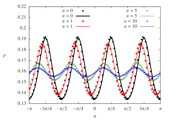
Figure 1: (Colour online) Invariant distribution $\rho(\theta)$ for various values of $\varkappa$. The points represent the numerically computed invariant distribution, while the lines correspond to Eq. (32).

Fig. 1 confirms that the invariant distribution is not uniform in the neighbourhood of the band centre. The amplitude of the modulation is largest at the exact band centre, i.e., for $\varkappa=0$, and gradually decreases as as the energy moves away from the band centre (i.e., for increasing values of $|\varkappa|$).

The numerical data displayed in Fig. 1 were obtained for disorder strength $\sigma^{2}=0.01$, but the results are the same for different values of $\sigma^{2}$. This is made evident by Fig. 2, which represents the invariant distribution of the map (16) at the band centre ($E=0$) computed for different values of the disorder strength. The good data collapse on the line corresponding to the theoretical form (32) confirms another feature of Eq. (32), i.e., that in the neighbourhood of the band centre the invariant distribution is determined by the parameter $\varkappa$ and does not depend on the disorder strength.

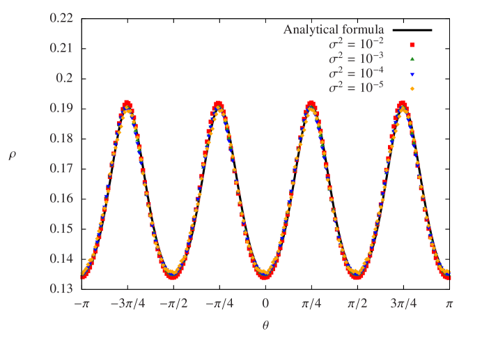
Figure 2: (Colour online) Invariant distribution $\rho(\theta)$ at the band centre ($E=0$) for various values of $\sigma^{2}$. The points represent the numerically computed invariant distribution, while the solid line corresponds to Eq. (32).

The data in Fig. 2 were obtained for $\varkappa=0$ but the same collapse occurs also for non-vanishing values of $\varkappa$.

As mentioned before, the general expression (32) for the invariant distribution reduces to simpler forms in the limit cases $|\varkappa|\ll 1$ and $|\varkappa|\gg 1$, which are the only ones considered in the literature [8, 11]. We devote the rest of this Section to the analysis of these particular cases.

3.1 The invariant distribution for $|\varkappa|\ll 1$

In the limit case $|\varkappa|\ll 1$ one can expand both the expression (32) and the normalisation factor (33) in powers of $\varkappa$. Carrying out the calculations, one eventually obtains that the limit form of the invariant distribution is

$$\rho(\theta)=\frac{2\rho(0)}{\sqrt{3+\cos(4\theta)}}\left\{1+\varkappa\left[-8F(\theta)+8\sqrt{\pi}\frac{\Gamma\left(\frac{3}{4}\right)}{\Gamma\left(\frac{1}{4}\right)}\int_{0}^{\theta}\frac{1}{\sqrt{3+\cos(4\phi)}}\mathrm{d}\phi\right]+O(\varkappa^{2})\right\}$$ (38)

with the constant factor $2\rho(0)$ given by

$$\begin{array}[]{ccl}2\rho(0)&=&\displaystyle\sqrt{\frac{2}{\pi}}\frac{\Gamma\left(\frac{3}{4}\right)}{\Gamma\left(\frac{1}{4}\right)}\left\{1+\varkappa\left[8\sqrt{\frac{2}{\pi}}\frac{\Gamma\left(\frac{3}{4}\right)}{\Gamma\left(\frac{1}{4}\right)}\int_{0}^{2\pi}\frac{F(\phi)}{\sqrt{3+\cos(4\phi)}}\mathrm{d}\phi\right.\right.\\ &-&\displaystyle\left.\left.8\sqrt{\frac{2}{\pi}}\left[\frac{\Gamma\left(\frac{3}{4}\right)}{\Gamma\left(\frac{1}{4}\right)}\right]^{2}\int_{0}^{2\pi}\frac{1}{\sqrt{3+\cos(4\theta)}}\int_{0}^{\theta}\frac{1}{\sqrt{3+\cos(4\phi)}}\mathrm{d}\phi\mathrm{d}\theta\right]\right\}+O(\varkappa^{2}).\end{array}$$

Eq. (38) coincides with the corresponding result first obtained by Derrida and Gardner [8]; the apparent difference is due to the election of these authors of a complex representation for the function (31).

At the band centre, i.e., for $\varkappa=0$, expression (38) reduces to the form

$$\rho(\theta)=\sqrt{\frac{2}{\pi}}\frac{\Gamma\left(\frac{3}{4}\right)}{\Gamma\left(\frac{1}{4}\right)}\frac{1}{\sqrt{3+\cos(4\theta)}}=\frac{1}{2\mathbf{K}\left(\frac{1}{\sqrt{2}}\right)\sqrt{3+\cos(4\theta)}}.$$

In the previous equation the symbol $\mathbf{K}(k)$ stands for the complete elliptic integral of the first kind,

$$\mathbf{K}(k)=\int_{0}^{\pi/2}\frac{d\phi}{\sqrt{1-k^{2}\sin^{2}\phi}}$$

and we used the identity

$$\mathbf{K}\left(\frac{1}{\sqrt{2}}\right)=\sqrt{\frac{\pi}{8}}\frac{\Gamma\left(\frac{1}{4}\right)}{\Gamma\left(\frac{3}{4}\right)}.$$

3.2 The invariant distribution for $|\varkappa|\gg 1$

We now consider the case $|\varkappa|\gg 1$. In this limit, the asymptotic expansion of $\rho(\theta)$ is obtained with less effort taking as a starting point the differential equation (28), rather than the general form (32) of the invariant distribution. After writing Eq. (28) as

$$\frac{d}{d\theta}\left[\rho(\theta)-\frac{1}{4\varkappa}\sin(4\theta)\rho(\theta)+\frac{1}{8\varkappa}\left(3+\cos(4\theta)\right)\frac{d\rho}{d\theta}\right]=0,$$ (39)

one can expand the solution in powers of $1/\varkappa$,

$$\rho(\theta)=\rho^{(0)}(\theta)+\frac{1}{\varkappa}\rho^{(1)}(\theta)+\frac{1}{\varkappa^{2}}\rho^{(2)}(\theta)+\ldots$$ (40)

Substituting the expansion (40) in Eq. (39) one obtains the hierarchy of equations

$$\frac{d\rho^{(0)}}{d\theta}=0$$ (41)

and

$$\frac{d}{d\theta}\left[\rho^{(n)}-\frac{1}{4}\sin(4\theta)\rho^{(n-1)}+\frac{1}{8}\left(3+\cos(4\theta)\right)\frac{d\rho^{(n-1)}}{d\theta}\right]=0$$ (42)

with $n=1,2,\ldots$ For the expansion (40) to satisfy the condition of periodicity and normalisation, the solution of Eq. (41) must be $2\pi$-periodic and normalised, while the solutions of the higher-order equations (42) must be $2\pi$-periodic and satisfy the conditions

$$\int_{0}^{2\pi}\rho^{(n)}(\theta)\mathrm{d}\theta=0.$$

In this way one can easily obtain that the behaviour of the invariant distribution for $\varkappa\gg 1$ is

$$\rho(\theta)=\frac{1}{2\pi}+\frac{1}{\varkappa}\frac{1}{8\pi}\sin(4\theta)-\frac{1}{\varkappa^{2}}\frac{3}{16\pi}\left[\cos(4\theta)+\frac{1}{4}\cos(8\theta)\right]+O\left(\frac{1}{\varkappa^{3}}\right).$$ (43)

Eq. (43) coincides with the result previously obtained in [8]. Note that as $|\varkappa|$ increases, i.e., as the energy moves away from the band centre, the invariant distribution tends to recover its flat form. The uniform limit, however, is reached with power-law convergence: this implies that the transition from anomalous to regular behaviour is smeared out over a wide energy range.

4 The localisation length

Having obtained the invariant distribution (32), one can compute the rhs of expression (19). After observing that the average of $\cos(2\theta)$ vanishes because the invariant distribution has period $\pi/2$, one obtains that the inverse localisation length is equal to

$$\begin{array}[]{ccl}\lambda&\simeq&\displaystyle\frac{\sigma^{2}}{8\left(1+\frac{E^{2}}{4}\right)}\left\{1+\frac{1}{N(\varkappa)}\int_{0}^{2\pi}\frac{\cos(4\theta)}{\sqrt{3+\cos(4\theta)}}e^{-8\varkappa F(\theta)}\right.\\ &\times&\displaystyle\left.\left[e^{4\sqrt{2}\pi\varkappa}\int_{0}^{\theta}\frac{e^{8\varkappa F(\phi)}}{\sqrt{3+\cos(4\phi)}}\mathrm{d}\phi+\int_{\theta}^{2\pi}\frac{e^{8\varkappa F(\phi)}}{\sqrt{3+\cos(4\phi)}}\mathrm{d}\phi\right]\mathrm{d}\theta\right\}.\end{array}$$ (44)

The general expression (44) is the central result of this paper. Its absence from previous works on the band-centre anomaly is probably explained by the fact that in the literature only the limit cases $|\varkappa|\ll 1$ and $|\varkappa|\gg 1$ have received attention so far. We discuss these limit cases below; we would like to emphasise, however, that only the general expression (44) makes possible to describe the behaviour of the localisation length over the whole range of the parameter $\varkappa$.

A remark is in order here. Because the invariant distribution (32) was obtained under the assumption $E\simeq-2\delta\to 0$, in the energy range where Eq. (44) is rigorously valid, it is equivalent to the following form

$$\begin{array}[]{ccl}\lambda&\simeq&\displaystyle\frac{\sigma^{2}}{8}\left\{1+\frac{1}{N(\varkappa)}\int_{0}^{2\pi}\frac{\cos(4\theta)}{\sqrt{3+\cos(4\theta)}}e^{-8\varkappa F(\theta)}\right.\\ &\times&\displaystyle\left.\left[e^{4\sqrt{2}\pi\varkappa}\int_{0}^{\theta}\frac{e^{8\varkappa F(\phi)}}{\sqrt{3+\cos(4\phi)}}\mathrm{d}\phi+\int_{\theta}^{2\pi}\frac{e^{8\varkappa F(\phi)}}{\sqrt{3+\cos(4\phi)}}\mathrm{d}\phi\right]\mathrm{d}\theta\right\}.\end{array}$$ (45)

which is obtained by setting $E=0$ in Eq. (44). However, as discussed below, we have found that Eq. (44) has a validity of its own because it provides a very effective interpolation between formula (45), which is applicable in a neighbourhood of the band centre, and Thouless’ expression (21) which can be used in the rest of the band (with the exception of the band edges).

It is not difficult to evaluate numerically Eq. (45); this operation makes possible to compare analytical and numerical results for the inverse localisation length. As shown by Fig. 3, the theoretical predictions of Eq. (45) fit very well the numerical data in a neighbourhood of the band centre.

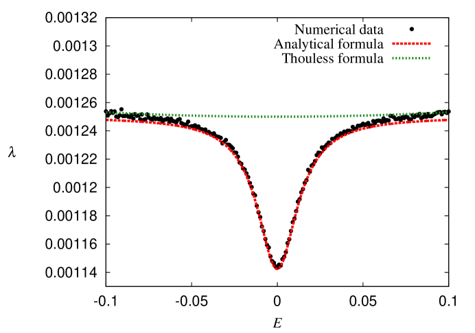
Figure 3: (Colour online) Inverse localisation length $\lambda$ versus energy $E$. The dots represent numerically computed values of the Lyapunov exponent; the dashed line is given by Eq. (45); the dotted line corresponds to Thouless’ formula.

For the case represented in Fig. 3 the disorder strength was set at $\sigma^{2}=0.01$; the considered energy interval $[-0.1,0.1]$ corresponds to values of $\varkappa$ in the range $[-10,10]$. It is easy to notice that the actual localisation length exhibits a non-negligible difference from the values predicted by Thouless’ formula even for energies lying quite away from the band centre. This is a consequence of the slow convergence of the invariant distribution (43) to the uniform limit discussed in Sec. 3.2; we can conclude that the phenomenon of anomalous localisation is not restricted to an infinitesimal neighbourhood of the band centre, but can be detected over a finite interval of energy values.

A close examination of Fig. 3 shows that, for energies $|E|\gtrsim 0.05$, the numerical data tend to overlap with Thouless’ formula, while Eq. (45) flattens. This is due to the fact that, as $\varkappa$ increases, Eq. (45) tends to a constant limit (see Eq. (47) below). The physical reason is that Eq. (45) is valid only as $|E|\to 0$. It turns out, however, that Eq. (44) works very well over the whole energy band. This is born out by Fig. 4, which compares the numerical data both with Thouless’ formula (21) and with Eq. (44).

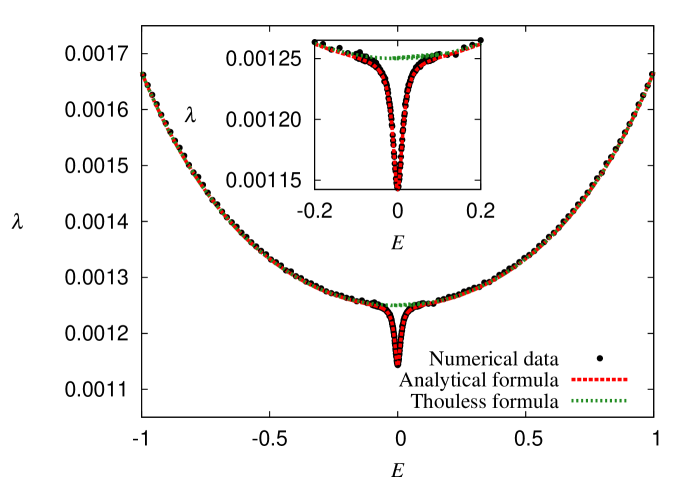
Figure 4: (Colour online) Inverse localisation length $\lambda$ versus energy $E$. The dots represent numerically computed values of the Lyapunov exponent; the dashed line is given by Eq. (44); the dotted line corresponds to Thouless’ formula. The inset shows in more detail the same data in the neighbourhood of the band centre.

That Eq. (44) works so well over the whole energy band is not surprising. In fact, the rhs of Eq. (44) is the product of Thouless’ formula and of a corrective factor. The latter is responsible for the anomalous behaviour of the localisation length in the neighbourhood of the band centre, but tends to unity for increasing values of $|E|$. In this way Thouless’ expression is recovered away from the band centre and the anomaly is taken into account by the corrective factor.

4.1 Localisation length for $|\varkappa|\ll 1$

We now turn our attention to the limit cases $|\varkappa|\ll 1$ and $|\varkappa|\gg 1$. In the case $|\varkappa|\ll 1$, i.e., when the energy lies very close to the band centre, one can evaluate the rhs of Eq. (19) with the approximate invariant distribution (38). In this way one obtains

$$\lambda=\sigma^{2}\left[\frac{\Gamma\left(\frac{3}{4}\right)}{\Gamma\left(\frac{1}{4}\right)}\right]^{2}\left[1+O(\varkappa)\right],$$ (46)

in agreement with the known result [8, 11, 18]. We remark that Eq. (46) can also be written in the equivalent form

$$\lambda=\frac{\sigma^{2}}{4}\left[2\frac{\mathbf{E}\left(\frac{1}{\sqrt{2}}\right)}{\mathbf{K}\left(\frac{1}{\sqrt{2}}\right)}-1\right]\left[1+O(\varkappa)\right]$$

which is sometimes used in the literature [7, 24]. The symbol $\mathbf{E}(k)$ represents the complete elliptic integral of the second kind, i.e.,

$$\mathbf{E}(k)=\int_{0}^{\pi/2}\sqrt{1-k^{2}\sin^{2}\phi}\;\mathrm{d}\phi.$$

4.2 Localisation length for $|\varkappa|\gg 1$

In the opposite case, i.e., for $|\varkappa|\gg 1$, the energy, although close to the band centre in absolute terms, moves away from it on the energy scale set by the strength of the disorder. When $|\varkappa|\gg 1$ the invariant distribution takes the form (43) and the inverse localisation length (45) becomes

$$\lambda=\frac{\sigma^{2}}{8}\left[1-\frac{3}{16\varkappa^{2}}+O\left(\frac{1}{\varkappa^{3}}\right)\right].$$ (47)

Once more, the result coincides with the formula first derived by Derrida and Gardner [8, 11].

In the limit $|\varkappa|\to\infty$ the inverse localisation length tends to the value predicted by Thouless’ formula (21); as already remarked the transition to the regular limit is not sharp because of the power-law decay of the anomalous term in the rhs of Eq. (47). It is important to remark, however, that the limit $|\varkappa|\to\infty$ in Eq. (47) can be taken only by letting the intensity of the disorder $\sigma^{2}$ tend to zero faster than the energy $E$. Simply increasing $|\varkappa|$ while keeping fixed the disorder strength eventually leads to the breakdown of the formula (47), which was derived under the assumption that $E\to 0$. This can be seen in Fig 3: for energies $|E|\gtrsim 0.05$ the inverse localisation length tends to move away from the anomalous expression (45) and closer to Thouless’ formula.

5 Conclusions

In this work we have analysed the anomalous localisation of the eigenstates of the 1D Anderson model for energies close to the band centre. Using the Hamiltonian map approach, we have derived two main results: the general expression (32) of the invariant distribution for the map (16) and the corresponding formula (44) for the inverse localisation length. The first result shows that the random phase approximation, which is an essential ingredient of the single-parameter scaling theory, fails close to the band centre. The failure is not restricted to a negligible energy range because the convergence of the distribution (32) to the uniform limit follows a power-law behaviour.

The invariant distribution (32) also allowed us to obtain the analytical expression (44) of the inverse localisation length. We have analytically proved that the general formula (44) describes the Kappus-Wegner anomaly around the band centre; because it reduces to Thouless’ formula when the energy moves away from the band centre, Eq. (44) works well over the whole energy band, as confirmed by the numerical data.

This paper provides new insight for a critical investigation of the SPS theory with the Hamiltonian map formalism. In this work we have focused our attention to the 1D map (16) for the angle variable and in this way we have been able to show that the random phase approximation, and hence the SPS theory, fail in a finite energy interval around the band centre. However, an extension of our analysis to the complete action-angle map given by Eqs. (16) and (17) is required in order to study the statistical properties of the conductance of a random segment. In fact, the conductance is related to the action variable, which is statistically correlated with the angle variable: hence a simultaneous study of both variables cannot be avoided. We plan to address this issue in a future work.

References

- [1] P. W. Anderson, Phys. Rev. 109, 1492 (1958)
- [2] K. Ishii, Suppl. Prog. Theor. Phys. 53, 77 (1973)
- [3] F. M. Izrailev, A. A. Krokhin, N. M. Makarov, arXiv:1110.1762
- [4] D. J. Thouless, p.1 in “La matière mal condensée - Ill-Condensed Matter”, R. Balian, R. Maynard, G. Toulouse eds., North-Holland (Amsterdam) and World Scientific (Singapore), 1979
- [5] G. Czycholl, B. Kramer, A. MacKinnon, Z. Phys. B 43, 5 (1981)
- [6] M. Kappus, F. Wegner, Z. Phys. B 45, 15 (1981)
- [7] S. Sarker, Phys. Rev. B 25, 4304 (1992)
- [8] B. Derrida, E. Gardner, J. Physique 45, 1283 (1984)
- [9] A. Bovier. A. Klein, J. Stat. Phys. 51, 501 (1988); M. Campanino, A. Klein, Comm. Math. Phys. 130, 441 (1990)
- [10] R. Kuske, Z. Scuss, I. Goldhirsch, S. H. Noskowicz, SIAM J. Appl. Math. 53, 1210 (1993)
- [11] I. Goldhirsch, S. H. Noskowicz, Z. Schuss, Phys. Rev. B 49, 14504 (1994)
- [12] H. Schomerus, M. Titov, Phys. Rev. B 67, 100201(R) (2003)
- [13] J. Heinrichs, J. Phys. C: Condens. Matter, 16, 7995 (2004)
- [14] L. I. Deych, A. A. Lisyansky, B. L. Altshuler, Phys. Rev. Lett. 84, 2678 (2000); L. I. Deych, M. V. Erementchouk, A. A. Lisyansky, B. L. Altshuler, Phys. Rev. Lett. 91, 096601 (2003)
- [15] E. Abrahams, P. W. Anderson, D. C. Licciardello, T. V. Ramakrishnan, Phys. Rev. Lett. 42, 673 (1979)
- [16] P. W. Anderson, D. J. Thouless, E. Abrahams, D. S. Fischer, Phys. Rev. B, 22, 3519 (1980)
- [17] F. M. Izrailev, T. Kottos, G. Tsironis, Phys. Rev. B 52, 3274 (1995)
- [18] F. M. Izrailev, S. Ruffo, L. Tessieri, J. Phys. A: Math. Gen. 31, 5263 (1998)
- [19] L. Tessieri, F. M. Izrailev, Phys. Rev. E 62, 3090 (2000); L. Tessieri, F. M. Izrailev, Phys. Rev. E 64, 066120 (2001)
- [20] C. J. Lambert, M. F. Thorpe, Phys. Rev. B 26, 4742 (1982); A. D. Stone, D. C. Allan, J. D. Joannopoulos, Phys. Rev. B 27, 836 (1983)
- [21] Kai Kang, Shaojing Qin, Chuilin Wang, Phys. Lett. A 375, 3529 (2011)
- [22] G. H. Hardy, E. M. Wright, An Introduction to the Theory of Numbers, 4th ed., Oxford University Press, Oxford (1960)
- [23] C. W. Gardiner, Handbook of Stochastic Methods, 3rd ed., Springer Verlag, Berlin (2004)
- [24] E. N. Economou, Green’s Functions in Quantum Physics, 3rd ed., Springer, Berlin (2006)