Counting free fermions on a line: a Fisher–Hartwig asymptotic expansion for the Toeplitz determinant in the double-scaling limit

Abstract

We derive an asymptotic expansion for a Wiener–Hopf determinant arising in the problem of counting one-dimensional free fermions on a line segment at zero temperature. This expansion is an extension of the result in the theory of Toeplitz and Wiener–Hopf determinants known as the generalized Fisher–Hartwig conjecture. The coefficients of this expansion are conjectured to obey certain periodicity relations, which renders the expansion explicitly periodic in the “counting parameter”. We present two methods to calculate these coefficients and verify the periodicity relations order by order: the matrix Riemann–Hilbert problem and the Painlevé V equation. We show that the expansion coefficients are polynomials in the counting parameter and list explicitly first several coefficients.

I Introduction and motivation

Toeplitz determinants are determinants of matrices whose elements depend only on the difference of the matrix indices:

$$D_{N}=\det_{1\leq i,j\leq N}a_{i-j}\,.$$ (1)

They occur in many topics of theoretical physics: statistical physics 1963-MPW ; 2006-Basor , random-matrix theory 1993-TracyWidom ; 1994-Widom , full counting statistics of fermionic systems 2011-AIQ , non-equilibrium bosonization 2010-GutmanGefenMirlin , etc. Typically, in physical applications, one is interested in the behaviour of a Toeplitz determinant (1) as the matrix size $N$ tends to infinity. For rapidly decaying matrix elements $a_{i-j}$, the leading exponential dependence of $D_{N}$ on $N$ can be easily understood on physical grounds: the coefficient in the exponent is given by the average logarithm of the “symbol” (the Fourier transform of $a_{i-j}$) of the Toeplitz matrix:

$$D_{N}\sim A\,\exp\left[N\oint\frac{dk}{2\pi}\ln\sigma(k)\right]\,,\qquad\sigma(k)=\sum_{m=-\infty}^{+\infty}a_{m}e^{-ikm}\,.$$ (2)

This result is known as the strong Szegő theorem BoettcherSilbermann-book ; 1952-Szego [the theorem also gives the coefficient $A$ in terms of $\sigma(k)$]. If the matrix elements $a_{i-j}$ decay slowly (or, equivalently, if the symbol $\sigma(k)$ has singularities), the exponential dependence (2) is complemented by power-law prefactors: the result known as the Fisher–Hartwig formula 1968-FisherHartwig ; 1978-Basor ; 1991-BasorTracy ; 2001-Ehrhardt ; BoettcherSilbermann-book ; 2010-DeiftItsKrasovsky ; 2010-Krasovsky .

A particularly interesting feature of the Fisher–Hartwig formula comes from the ambiguity in choosing the branch of the logarithm in Eq. (2) in the case of a singular $\sigma(k)$. As a result, one obtains multiple branches of the asymptotic dependence of $D_{N}$ on $N$, and the traditional Fisher–Hartwig formula prescribes selecting the leading one (having the prefactor with the largest power of $N$). If the Toeplitz matrix depends on a parameter, the leading branch may switch as a function of this parameter: in this case, the asymptotic behavior of $D_{N}$ depends on it nonanlytically. At the switching point, two branches are equally relevant, and the correct asymptotic behavior is given in this case by a simple sum of these two branches. This prescription known as the generalized Fisher–Hartwig conjecture 1991-BasorTracy was recently proven in Ref. 2010-DeiftItsKrasovsky, .

In recent literature, it was conjectured that subleading branches of the Fisher–Hartwig formula do not need to be discarded, but they provide an accurate description of subleading terms in an asymptotic expansion of $D_{N}$ as $N$ tends to infinity 2005-FranchiniAbanov ; 2011-GutmanGefenMirlin ; 2010-CalabreseEssler ; 2009-Kitanine-2 . Moreover, each of the Fisher–Hartwig branches (2) may, in turn, be improved by including corrections as a usual power series in $1/N$. It was further conjectured that a full asymptotic series for $D_{N}$ may be obtained as the sum of all Fisher–Hartwig branches, in which all terms in the $1/N$ expansion are kept 2009-Kitanine ; 2008-Kozlowski . A particular case of this conjecture was also proposed in Ref. 2011-AIQ, for the Toeplitz determinant describing the full counting statistics of one-dimensional free fermions. It was verified numerically that, in this example, the first subleading $1/N$ terms in the leading and subleading Fisher–Hartwig branches reproduce several terms in an asymptotic expansion of $D_{N}$.

In this work, we support this conjecture by an explicit calculation for the problem of free fermions on a continuous line, which is a limiting case of the lattice model considered in Ref. 2011-AIQ, . In this limit, $N$ is replaced by a continuous parameter $x$, the Toeplitz determinant becomes a Fredholm determinant (more specifically, a Wiener–Hopf determinant with a piecewise constant symbol 1983-BasorWidom ; 1994-BoettcherSilbermannWidom ), and we may use methods developed for the latter 1980-JMMS ; 1993-TracyWidom ; KorepinEtAl-book ; 2003-ChZ . We derive a complete asymptotic expansion consistent with the above-mentioned genrealization of the Fisher–Hartwig conjecture. A proof of this new conjecture is still missing: it amounts to certain “periodicity relations” on the coefficients of this expansion. However, we present a systematic algorithm for calculating the coefficients to an arbitrarily high order in $1/x$, which allows us to verify these periodicity relations order by order. We have verified the periodicity relations up to the 15th order in $1/x$, and conjecture that they hold to all orders.

II Formulation of the problem

We begin our definitions with a description of a relevant physical problem of full counting statistics of free fermions on a segment of an infinite line. Consider free fermions in one dimension at zero temperature. Their multi-particle state is characterized by a single parameter: the wave vector $k_{F}$ such that all states with wave vectors $|k|<k_{F}$ are filled and all states with $|k|>k_{F}$ are empty. We are interested in the expectation value $\langle\exp[2\pi i\kappa\hat{Q}]\rangle$, where $\hat{Q}$ is the operator of the number of particles on a given line segment of length $L$ and $\kappa$ is an auxiliary “counting parameter” 1993-LevitovLesovik ; 2011-AIQ ; 1990-Its ; note-kappa . This expectation value may be re-expressed as a determinant of a single-particle operator 2002-Klich ; 2009-AI ; 2011-AIQ ; KorepinEtAl-book :

$$\langle\exp[2\pi i\kappa\hat{Q}]\rangle=\det\left[1+n_{F}\left(e^{2\pi i\kappa Q}-1\right)\right]=\det\left[1+n_{F}Q\left(e^{2\pi i\kappa}-1\right)\right]\,.$$ (3)

Here $Q$ in the right-hand side is the single-particle projector on the line segment in real space,

$$Q=\begin{cases}1&\text{if $0<q<L$}\,,\\ 0&\text{otherwise}\end{cases}$$ (4)

($q$ is the coordinate on the line) and $n_{F}$ is the projector on the occupied states in the Fourier space,

$$n_{F}=\begin{cases}1&\text{if $|k|<k_{F}$}\,,\\ 0&\text{otherwise}\,.\end{cases}$$ (5)

The determinant (3) is of the Wiener–Hopf type 1983-BasorWidom ; 1994-BoettcherSilbermannWidom . It may be understood as a Fredholm determinant,

$$\det\left[1+n_{F}Q\left(e^{2\pi i\kappa}-1\right)\right]=\sum_{l=0}^{\infty}\frac{(e^{2\pi i\kappa}-1)^{l}}{l!}\int_{0}^{L}dq_{1}\ldots\int_{0}^{L}dq_{l}\det_{1\leq i,j\leq l}\left[n_{F}(q_{i}-q_{j})\right]\,,$$ (6)

where $n_{F}(q_{i}-q_{j})$ is the Fourier transform of $n_{F}$ defined by Eq. (5):

$$n_{F}(q)=\frac{\sin(k_{F}q)}{\pi q}\,.$$ (7)

Obviously, the determinant (6) depends on $k_{F}$ and $L$ only via their product $k_{F}L$, and therefore we may define

$$\chi(\kappa,x)=\det\left[1+n_{F}Q\left(e^{2\pi i\kappa}-1\right)\right]\,,\qquad x=k_{F}L\,.$$ (8)

Alternatively, we may define the same function $\chi(\kappa,x)$ by discretizing the space coordinate $q$ and then taking the continuous limit (as in Ref. 2011-AIQ, ). Namely, we may first consider the Toeplitz determinant on a lattice:

$$D_{N}(\kappa,k_{F})=\det_{1\leq i,j\leq N}\left[\delta_{ij}+n_{F}(i-j)\left(e^{2\pi i\kappa}-1\right)\right]$$ (9)

[here $n_{F}(i-j)$ is defined by the same expression (7) with $n_{F}(0)=k_{F}/\pi$] and then define the function $\chi(\kappa,x)$ as the limit

$$\chi(\kappa,x)=\lim_{N\to\infty}D_{N}(\kappa,x/N)$$ (10)

This type of definition is refered to as a “double-scaling limit” in Ref. 2010-Krasovsky, .

We have thus defined a function of two variables $\chi(\kappa,x)$. At a given $x$, it is periodic in $\kappa$ with period one. From the expansion (6) it follows that $\chi(\kappa,x)$ is an entire function of $\kappa$ at any fixed value of $x$. The main result of this paper is a conjecture of an explicitly periodic asymptotic expansion for $\chi(\kappa,x)$ at $x\to\infty$, Eqs. (11) and (12). As announced in the introduction, the leading asymptotics of $\chi(\kappa,x)$ at $x\to\infty$ is discontinuous in $\kappa$ (at points $\operatorname{Re}(\kappa)=l+1/2$ with integer $l$), and our asymptotic expansion describes in full detail the development of this discontinuity related to the switching of Fisher–Hartwig branches.

III Main results

In Section IV below, we derive the asymptotic expansion (34) for the function $\chi(\kappa,x)$. This form of the asymptotic expansion is proven, provided $\operatorname{Re}(\kappa)\neq l+1/2$ for any integer $l$, and the coefficients $L_{j}(\kappa,x)$ are computable, as Laurent series in $1/x$, iteratively order by order.

Furthermore, we conjecture that the coefficients $L_{j}(\kappa,x)$ obey the “periodicity relations” (35), which brings the expansion (34) to an explicitly periodic form. Under this assumption (which we verified to many orders in $1/x$), the expansion (34) may be brought to the form

$$\chi(\kappa,x)=\sum_{j=-\infty}^{+\infty}\chi_{*}(\kappa+j,x)\,,$$ (11)

where

$$\chi_{*}(\kappa,x)=\exp\left[2i\kappa x-2\kappa^{2}\ln x+C(\kappa)+\sum_{n=1}^{\infty}f_{n}(\kappa)\,(ix)^{-n}\right]\,.$$ (12)

This asymptotic expansion agrees with the general conjecture proposed in Refs. 2009-Kitanine, ; 2008-Kozlowski, and with a more explicit formula conjectured in Ref. 2011-AIQ, .

The sum in Eq. (11) corresponds to adding together all different Fisher–Hartwig branches, and the sum in Eq. (12) includes all $(1/x)^{n}$ corrections within a given branch. The coefficient $C(\kappa)$ is given by 1983-BasorWidom ; 1994-BoettcherSilbermannWidom ; 2003-ChZ ; 2011-AIQ :

$$C(\kappa)=2\ln\left[G(1+\kappa)G(1-\kappa)\right]-2\kappa^{2}\ln 2\,,$$ (13)

where $G(z)$ is the Barnes $G$ function BarnesG . The coefficients $f_{n}(\kappa)$ are polynomials in $\kappa$ with real rational coefficients, and they are odd/even in $\kappa$ at odd/even $n$, respectively. Moreover, the lowest power of $\kappa$ in $f_{n}(\kappa)$ is 3 or 4 (for $n$ odd or even, respectively) note-degree . The first several coefficients are note-F1 :

$$f_{1}(\kappa)=2\kappa^{3}\,,$$

$$f_{2}(\kappa)=\frac{5}{2}\kappa^{4}\,,$$

$$f_{3}(\kappa)=\frac{11}{2}\kappa^{5}+\frac{1}{6}\kappa^{3}\,,$$

$$f_{4}(\kappa)=\frac{63}{4}\kappa^{6}+\frac{13}{8}\kappa^{4}\,,$$ (14)

$$f_{5}(\kappa)=\frac{527}{10}\kappa^{7}+12\kappa^{5}+\frac{1}{5}\kappa^{3}\,,$$

$$f_{6}(\kappa)=\frac{3129}{16}\kappa^{8}+\frac{1931}{24}\kappa^{6}+\frac{75}{16}\kappa^{4}\,,$$

$$f_{7}(\kappa)=\frac{175045}{224}\kappa^{9}+\frac{8263}{16}\kappa^{7}+\frac{2155}{32}\kappa^{5}+\frac{45}{56}\kappa^{3}\,.$$

In Sections IV and V we give algorithms for calculating the coefficients $f_{n}(\kappa)$ order by order up to an arbitrary large $n$.

In this work, we prove neither the expansion (11)–(12) nor even its weaker form (34) at points $\operatorname{Re}(\kappa)=l+1/2$. However we conjecture that it is also valid there, so that the expansion (11)–(12) is in fact a uniform asymptotic expansion on any compact subset of $\kappa$.

IV Derivation using the matrix Riemann–Hilbert problem

In this section we show how the expansion (11), (12) can be derived by means of the asymptotic solution of the associated Riemann–Hilbert problem. The relationship between the the matrix Riemann–Hilbert problem, integrable partial differential equations and Fredholm determinants of integrable kernels, in particular the sine kernel, was exploited in different contexts such as classical inverse scattering problem, random matrix theory and quantum integrable systems 1990-Its ; 1990-ItsIzergin ; 1992-Its ; 1993-Its ; 1997-DeiftItsZhou ; 1998-Gohmann ; 2000-FujiiWadati ; 2001-Shiroishi ; 2003-ChZ . The asymptotic solution of the matrix Riemann–Hilbert problem for the generalized sine kernel with Hartwig–Fisher singularities was developed in Refs. 2003-ChZ, ; 2009-Kitanine, ; 2010-DeiftItsKrasovsky, . In this section we follow the notations of Ref. 2003-ChZ, . In that work, the logarithmic derivative of the function $\chi(\kappa,x)$ was expressed in terms of a solution of a certain Riemann–Hilbert matrix problem, and then this problem was solved to the leading order in $x$. In this section, we solve the same Riemann–Hilbert matrix problem in terms of a series in $1/x$ whose coefficients may be calculated iteratively, order by order.

We do not repeat here the full argument of Ref. 2003-ChZ, , but start with formulating their result relevant for our calculation. We refer the reader to the original paper for its derivation. The logarithmic derivative of $\chi(\kappa,x)$ was expressed there as

$$\frac{\partial}{\partial x}\ln\chi(\kappa,x)=2i\kappa-i\lim_{k\to\infty}k\left[S_{\infty}(k)_{11}-1\right]\,,$$ (15)

where $S_{\infty}(k)_{11}$ is the upper-left-corner matrix element of the $2\times 2$ matrix $S_{\infty}(k)$, which solves the Riemann–Hilbert problem (in the complex variable $k$) formulated below.

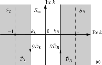
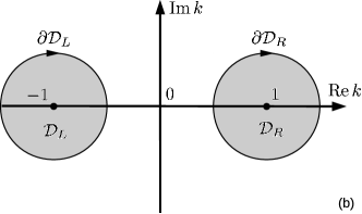
Figure 1: (a) Initial choice of domains for the matrix Riemann–Hilbert problem (21). The dashed lines denote the branch cuts of $\theta_{R}(k)$ in $\tilde{\cal D}_{R}$ and of $\theta_{L}(k)$ in $\tilde{\cal D}_{L}$. The arrows at the boundaries $\partial\tilde{\cal D}_{R,L}$ denote their orientation in the integral (30). (b) The choice of domains used in Ref. 2003-ChZ, and in our formula (33).

Define regions $\tilde{\cal D}_{R}$ and $\tilde{\cal D}_{L}$ as $\operatorname{Re}k>k_{R}$ and $\operatorname{Re}k<k_{L}$, respectively, where the region boundaries are chosen as $-1<k_{L}<k_{R}<1$ (see Fig. 1a). This choice of regions differs slightly from Ref. 2003-ChZ, , where the regions were chosen as discs around $k=\pm 1$: this difference does not change anything in our calculation, but simplifies the discussion of branch cuts. In these regions, we define the two matrix-valued functions:

$$\theta_{R}(k)=\left(\begin{array}[]{cc}\tilde{\Psi}[-\kappa,-ix(k-1)]&\displaystyle\frac{a_{R}[x(k+1)]^{-2\kappa}}{x(k-1)}\tilde{\Psi}[1+\kappa,ix(k-1)]\\ \displaystyle\frac{b_{R}[x(k+1)]^{2\kappa}}{x(k-1)}\tilde{\Psi}[1-\kappa,-ix(k-1)]&\tilde{\Psi}[\kappa,ix(k-1)]\end{array}\right)$$ (16)

in the region $\tilde{\cal D}_{R}$ and

$$\theta_{L}(k)=\left(\begin{array}[]{cc}\tilde{\Psi}[\kappa,ix(k+1)]&\displaystyle\frac{a_{L}[x(k-1)]^{2\kappa}}{x(k+1)}\tilde{\Psi}[1-\kappa,ix(k+1)]\\ \displaystyle\frac{b_{L}[x(k-1)]^{-2\kappa}}{x(k+1)}\tilde{\Psi}[1+\kappa,-ix(k+1)]&\tilde{\Psi}[-\kappa,-ix(k+1)]\end{array}\right)$$ (17)

in the region $\tilde{\cal D}_{L}$. Here the constants $a_{R}$ and $b_{R}$ are the same as in Ref. 2003-ChZ, ,

$$a_{R}=-\frac{i\pi e^{i\pi\kappa}e^{ix}}{\Gamma^{2}(-\kappa)}\,,\qquad b_{R}=-\frac{i\pi e^{-i\pi\kappa}e^{-ix}}{\Gamma^{2}(\kappa)\sin^{2}(\pi\kappa)}\,,$$ (18)

the coefficients $a_{L}$ and $b_{L}$ are defined as

$$b_{L}=-\frac{a_{R}}{\sin^{2}(\pi\kappa)}\,,\qquad a_{L}=-b_{R}\sin^{2}(\pi\kappa)\,,$$ (19)

and we have introduced a shorthand notation

$$\tilde{\Psi}(a,w)=w^{a}\Psi(a,1;w)\,,$$ (20)

where $\Psi(a,1;w)$ is the Tricomi function 1953-BatemanErdelyi . The functions $\Psi(a,1;w)$ and $\tilde{\Psi}(a,w)$ are defined to have branch-cut discontinuities along the negative real axis $w\in{{\mathbb{R}}}_{-}$. Then the matrices $\theta_{R}(k)$ and $\theta_{L}(k)$ have discontinuities along the lines $\operatorname{Re}k=\pm 1$, respectively. Note however that those discontinuities decay exponentially in $|x(k\mp 1)|$, so that $\theta_{R}(k)$ and $\theta_{L}(k)$ have regular asymptotic expansions in inverse powers of $x(k\mp 1)$ (see Ref. 2003-ChZ, for more detail). We now formulate the Riemann–Hilbert problem for a matrix $S(k)$:

$${\rm(i)~{}~{}} S(k){\rm~{}~{}is~{}analytic~{}in~{}~{}}{{\mathbb{C}}}\backslash(\partial\tilde{\cal D}_{R}\cup\partial\tilde{\cal D}_{L})\,;$$

$${\rm(ii)~{}~{}} S_{\infty}(k)=S_{R,L}(k)\theta_{R,L}{\rm~{}at~{}}k\in\partial\tilde{\cal D}_{R,L}\,;$$ (21)

$${\rm(iii)~{}~{}} S_{\infty}(k)\to I{\rm~{}~{}as~{}~{}}k\to\infty\,,$$

where we denote by $S_{R,L,\infty}$ the restrictions of $S(k)$ onto $\tilde{\cal D}_{R}$, $\tilde{\cal D}_{L}$, and ${{\mathbb{C}}}\backslash(\tilde{\cal D}_{R}\cup\tilde{\cal D}_{L})$, respectively. The matrix $S_{\infty}(k)$ obtained as a solution to this Riemann–Hilbert problem can be then used to find the logarithmic derivative of $\chi(\kappa,x)$, according to Eq. (15). This relation is exact and is a minor reformulation of results obtained in Sections 3 and 4 of Ref. 2003-ChZ, .

We can now calculate the asymptotic expansion for $S_{\infty}(k)$ by expanding $\theta_{R,L}$ in powers of $1/x$ and matching the matrix at the contours $\partial\tilde{\cal D}_{R,L}$ order by order. In this expansion, we will treat all powers of $x^{\kappa}$ and of $e^{ix}$ as terms of order zero with respect to $x$: in other words, we will collect together all terms with the same integer powers of $x$, while letting the coefficients to depend on $x^{\kappa}$ and $e^{ix}$. As we shall see below, such a method indeed produces an asymptotic expansion for $S_{\infty}(k)$ within the interval $|\operatorname{Re}(\kappa)|<1/2$.

We start with the (asymptotic) expansion

$$\tilde{\Psi}(a,w)=\sum_{n=0}^{\infty}\frac{p_{n}(a)}{w^{n}}\,,\qquad{\rm where}\qquad p_{n}(a)=\frac{(-1)^{n}}{n!}a^{2}(a+1)^{2}\ldots(a+n-1)^{2}$$ (22)

to expand

$$\theta_{R,L}=I+\frac{1}{x}\theta_{R,L}^{(1)}+\frac{1}{x^{2}}\theta_{R,L}^{(2)}+\ldots\,,$$ (23)

where

$$\theta_{R}^{(n)}=\frac{1}{(k-1)^{n}}\left(\begin{array}[]{cc}i^{n}p_{n}(-\kappa)&(-i)^{n-1}a_{R}p_{n-1}(1+\kappa)\left[x(k+1)\right]^{-2\kappa}\\ i^{n-1}b_{R}p_{n-1}(1-\kappa)\left[x(k+1)\right]^{2\kappa}&(-i)^{n}p_{n}(\kappa)\end{array}\right)$$ (24)

and

$$\theta_{L}^{(n)}=\frac{1}{(k+1)^{n}}\left(\begin{array}[]{cc}i^{n}p_{n}(\kappa)&(-i)^{n-1}a_{L}p_{n-1}(1-\kappa)\left[x(k-1)\right]^{2\kappa}\\ i^{n-1}b_{L}p_{n-1}(1+\kappa)\left[x(k-1)\right]^{-2\kappa}&(-i)^{n}p_{n}(-\kappa)\end{array}\right)$$ (25)

(note that $\theta_{L,R}^{(n)}$ depend on $x$ themselves, but only “weakly”, via $x^{\pm 2\kappa}$).

Now the Riemann–Hilbert problem (21) may be solved iteratively (order by order) in terms of an expansion

$$S(k)=I+\frac{1}{x}S^{(1)}(k)+\frac{1}{x^{2}}S^{(2)}(k)+\ldots\,,$$ (26)

where $S^{(n)}(k)$ are polynomials in $x^{\pm 2\kappa}$. Note that this method slightly differs from the approach used in Ref. 2003-ChZ, , where the ansatz (3.53) allowed to partly resum the series (26). We denote the functions $S^{(n)}$ in the three domains $\tilde{\cal D}_{R}$, $\tilde{\cal D}_{L}$, and ${{\mathbb{C}}}\backslash(\tilde{\cal D}_{R}\cup\tilde{\cal D}_{L})$ by $S_{R}^{(n)}$, $S_{L}^{(n)}$, and $S_{\infty}^{(n)}$, respectively. To the first order, we find

$$S_{\infty}^{(1)}(k)=S_{R,L}^{(1)}(k)+\theta_{R,L}^{(1)}(k)\quad{\rm at}\quad k\in\partial\tilde{\cal D}_{R,L}\,,$$ (27)

while the general equation at the $n$-th order is

$$S^{(n)}_{\infty}(k)=S^{(n)}_{R,L}(k)+S^{(n-1)}_{R,L}(k)\theta^{(1)}_{R,L}(k)+\ldots+S^{(1)}_{R,L}(k)\theta^{(n-1)}_{R,L}(k)+\theta^{(n)}_{R,L}(k)\quad{\rm at}\quad k\in\partial\tilde{\cal D}_{R,L}\,.$$ (28)

Using the analyticity of $S_{R}^{(n)}$, $S_{L}^{(n)}$, and $S_{\infty}^{(n)}$ in the domains $\tilde{\cal D}_{R}$, $\tilde{\cal D}_{L}$, and ${{\mathbb{C}}}\backslash(\tilde{\cal D}_{R}\cup\tilde{\cal D}_{L})$, respectively, and the boundary condition $S^{(n)}_{\infty}(k)\to 0$ at $k\to\infty$, we can solve these equations by the Cauchy integral formula. At the first order, solving Eq. (27), we find

$$S^{(1)}(k)=\oint_{\partial\tilde{\cal D}_{R}}\frac{dk^{\prime}}{2\pi i}\frac{1}{k^{\prime}-k}\theta^{(1)}_{R}(k^{\prime})+\oint_{\partial\tilde{\cal D}_{L}}\frac{dk^{\prime}}{2\pi i}\frac{1}{k^{\prime}-k}\theta^{(1)}_{L}(k^{\prime})$$ (29)

and, more generally, at the $n$-th order, the solution to Eq. (28) reads

$$S^{(n)}(k)=\sum_{\alpha=R,L}\oint_{\partial\tilde{\cal D}_{\alpha}}\frac{dk^{\prime}}{2\pi i}\frac{1}{k^{\prime}-k}\left[S^{(n-1)}_{\alpha}(k^{\prime})\theta^{(1)}_{\alpha}(k^{\prime})+\ldots+S^{(1)}_{\alpha}(k^{\prime})\theta^{(n-1)}_{\alpha}(k^{\prime})+\theta^{(n)}_{\alpha}(k^{\prime})\right]\,.$$ (30)

These formulas produce the components $S_{\infty}^{(n)}(k)$, $S_{R}^{(n)}(k)$, and $S_{L}^{(n)}(k)$ depending on the location of the point $k$. At this stage of the calculation, it is technically convenient to deform the integration contours $\partial\tilde{\cal D}_{\alpha}$ into the boudaries $\partial{\cal D}_{\alpha}$ of some nonoverlapping discs ${\cal D}_{R}$ and ${\cal D}_{L}$ centered at $k=1$ and $k=-1$, respectively, as in Ref. 2003-ChZ, (See Fig. 1b). This deformation is allowed, since the ingtegrations converge rapidly at infinity and the cuts of the matrix functions $\theta_{R,L}(k)$ disappear from the asymptotic expansion.

The formula (30), in principle, solves our problem: knowing the expansions (24) and (25), we iteratively calculate $S^{(n)}(k)$ from (30) and then extract the logarithmic derivative of $\chi(\kappa,x)$ using (15). As a result, we obtain the asymptotic series note-expansion

$$\frac{\partial}{\partial x}\ln\chi(\kappa,x)=2i\kappa+\sum_{n=1}^{\infty}I_{n}(\kappa,x)\,,$$ (31)

where

$$I_{n}(\kappa,x)=\sum_{m}R_{n,m}(\kappa)\,x^{-n-4m\kappa}e^{2imx}$$ (32)

is the contribution from $S_{\infty}^{(n)}(k)$. The form (32) of the term $I_{n}(\kappa,x)$ follows from examining the explicit expression

$$I_{n}(\kappa,x)=i\sum_{\begin{subarray}{c}\{n_{j}\}\\ n_{j}\geq 1\\ \sum_{j=1}^{s}n_{j}=n\end{subarray}}\sum_{\begin{subarray}{c}\{\alpha_{j}\}\\ \alpha_{j}=R,L\end{subarray}}\oint_{\partial D_{\alpha_{1}}^{[1]}}\frac{dk_{1}}{2\pi i}\ldots\oint_{\partial D_{\alpha_{s}}^{[s]}}\frac{dk_{s}}{2\pi i}\frac{1}{k_{1}-k_{2}}\cdots\frac{1}{k_{s-1}-k_{s}}\left[\theta_{\alpha_{1}}^{(n_{1})}(k_{1})\ldots\theta_{\alpha_{s}}^{(n_{s})}(k_{s})\right]_{11}\,,$$ (33)

which is obtained by an iterative application of Eq. (30). Here the sum is taken over all integer partitions of $n$ into the sum of $n_{j}$, and, for each such partition, over choices of the left and right integration contour for each $j$. Furthermore, the integration contours are ordered in such a way that the contour $\partial D_{\alpha}^{[j]}$ lies inside $\partial D_{\alpha}^{[j^{\prime}]}$, if $j>j^{\prime}$. Every integral in Eq. (33) can be easily calculated by residues. The coefficients $R_{n,m}(\kappa)$ can be easily extracted from this expression by selecting terms with a particular power of $x$. The following properties of these coefficients can be proven:

1. The coefficients $R_{n,m}(\kappa)$ vanish for $|m|>[n/2]$. This means that the sum over $m$ in Eq. (32) extends only from $-[n/2]$ to $+[n/2]$.

2. The coefficients $R_{n,m}(\kappa)$ have a definite parity: $R_{n,m}(-\kappa)=(-1)^{n-1}R_{n,-m}(\kappa)$. This follows from the symmetry $k\mapsto-k$ (see a detailed discussion of this symmetry in Section 3 of Ref. 2003-ChZ, ).

3. The coefficients $R_{n,0}(\kappa)$ are polynomials in $\kappa$ with real rational coefficients multiplied by $(-i)^{n+1}$. The smallest possible degree of $\kappa$ contained in this polynomial is 3 or 4, depending on the parity of $n$. This can be easily seen for every term in the sum (33) by using the identity $a_{R}b_{R}=a_{L}b_{L}=-\kappa^{2}$.

4. The first coefficient in the expansion (31) is $R_{1,0}(\kappa)=-2\kappa^{2}$ [calculated directly using the formula (33)].

Note that the powers of $x$ in the formal series (31)–(32) decay if and only if $|\operatorname{Re}(\kappa)|<1/2$. Therefore our calculation produces an asymptotic expansion for $(\partial/\partial x)\ln\chi(\kappa,x)$ only within this interval of values of $\kappa$.

To obtain the expansion of the function $\chi(\kappa,x)$, we integrate and then exponentiate the expansion (31), (32) as a formal series in $x^{-1}$. In the resulting series, we collect together terms with the same oscillatory prefactor $e^{2ijx}$. The result may be further written as

$$\chi(\kappa,x)=\sum_{j=-\infty}^{+\infty}\exp\left[2i(\kappa+j)x-2(\kappa+j)^{2}\ln x\right]L_{j}(\kappa,x)\,,$$ (34)

where $L_{j}(\kappa,x)$ are Laurent series in $x$ with coefficients depending on $\kappa$. These coefficients may be expressed in terms of $R_{n,m}$ and vice versa, modulo an overall numerical prefactor in all $L_{j}(\kappa,x)$, which is left undetermined [it corresponds to the integration constant of Eq. (31)].

It seems very plausible [and it was conjectured both in the Toeplitz (chain) and Wiener–Hopf (continuous) cases 2009-Kitanine ; 2008-Kozlowski ; 2011-AIQ ] that the expansion of the form (34) is explicitly periodic in $\kappa$, namely

$$L_{j}(\kappa,x)=L_{0}(\kappa+j,x)\,.$$ (35)

We do not have a proof of this conjecture at the moment, but we have verified it analytically up to the order $x^{-15}$ in Eq. (34) using the technique based on the Painllevé V equation, see Section V. We conjecture that the relations (35) hold to all orders.

Finally, we observe that $L_{0}(\kappa,x)$ does not contain negative powers of $x$ [and, under the periodicity conjecture (35), neither do any of $L_{j}(\kappa,x)$] and, therefore may be formally written as

$$L_{0}(\kappa,x)=\exp\left[C(\kappa)+\sum_{n=1}^{\infty}f_{n}(\kappa)(ix)^{-n}\right]$$ (36)

(we included the factors $i^{-n}$ in the expansion to make the coefficients real). Under the “periodicity conjecture” (35), this immediately leads to the perioduc form of the expansion (11)–(12).

The coefficient $C(\kappa)$ cannot be calculated by the method described, but it is known from other approaches 1983-BasorWidom ; 1994-BoettcherSilbermannWidom ; 2003-ChZ ; 2011-AIQ and is given by Eq. (13). To calculate the coefficients $f_{n}(\kappa)$, we relate them to $R_{n,m}(\kappa)$. In fact, it is sufficient to consider only the coefficients $R_{n,0}(\kappa)$. By comparing the expansion (31), (32) wtih (11) – (13), one finds:

$$R_{2,0}(\kappa)=-i^{-1}f_{1}(\kappa)\,,$$

$$R_{3,0}(\kappa)=-2i^{-2}f_{2}(\kappa)\,,$$

$$R_{4,0}(\kappa)=-3i^{-3}f_{3}(\kappa)\,,$$

$$R_{5,0}(\kappa)=-4i^{-4}\left[f_{4}(\kappa)-e^{\Delta_{0}}\right]\,,$$ (37)

$$R_{6,0}(\kappa)=-5i^{-5}\left[f_{5}(\kappa)-e^{\Delta_{0}}\Delta_{1}\right]\,,$$

$$R_{7,0}(\kappa)=-6i^{-6}\left[f_{6}(\kappa)-e^{\Delta_{0}}\left(\Delta_{2}+\frac{\Delta_{1}^{2}}{2}\right)\right]\,,$$

$$R_{8,0}(\kappa)=-7i^{-7}\left[f_{7}(\kappa)-e^{\Delta_{0}}\left(\Delta_{3}+\Delta_{2}\Delta_{1}+\frac{\Delta_{1}^{3}}{6}\right)\right]\,,$$

where we denote

$$e^{\Delta_{0}}=\exp\left[C(\kappa+1)+C(\kappa-1)-2C(\kappa)\right]=\frac{\kappa^{4}}{16}$$ (38)

and

$$\Delta_{n\geq 1}=f_{n}(\kappa+1)+f_{n}(\kappa-1)-2f_{n}(\kappa)\,.$$ (39)

Note that $R_{n,0}(\kappa)$ with $n>4$ contain cross terms (containing $\Delta_{n}$) arising from Fisher–Hartwig branches with $j\neq 0$ in Eq. (11). By explicitly calculating $R_{n,0}(\kappa)$ from Eq. (33) [we used a computer program to perform this calculation] and solving Eqs. (37), we arrive at the results (14). We also remark that, for large $n$, the use of the formula (33) is not practical for explicit calculations (the number of terms grows very rapidly with $n$), and Eq. (30) seems to be more efficient.

We can now prove the properties of the coefficients $f_{n}(\kappa)$ declared in Section III.

• The reality of $f_{n}(\kappa)$ follows from the property 3 of $R_{n,0}(\kappa)$: indeed, if we choose $(ix)$ as the expansion variable, then all the coefficients of the expansions become real.

• The parity of the coefficients $f_{n}(\kappa)$ follows from the parity of $R_{n,0}(\kappa)$ (property 2). One can also formulate this property as an invariance of the whole asymptotic series with respect to the simultaneous formal sign change of $x$ and $\kappa$ in their integer powers, while transforming fractional powers of $x$ as $x^{4\kappa}\mapsto x^{-4\kappa}$.

• One can also easily verify that the cross terms in relations (37), for any $R_{n,0}$, are always polynomials divisible by $\kappa^{4}$. Therefore the property that $R_{n,0}$ is always divisible by $\kappa^{3}$ also holds for $f_{n}(\kappa)$.

V Calculation using the Painlevé V equation

An alternative way to obtain the asymptotic expansion (11), (12) is the use of the Painlevé V equation. It was discovered in the seminal paper 1980-JMMS (with a simpler version of the derivation presented later in Ref. 1993-TracyWidom, ) that the Fredholm determinant (8) considered as a function of $x$ satisfies an ordinary differential equation: the Painlevé V equation in the Jimbo–Miwa form,

$$(x\sigma^{\prime\prime})^{2}+4(x\sigma^{\prime}-\sigma)\left(x\sigma^{\prime}-\sigma+(\sigma^{\prime})^{2}\right)=0\,.$$ (40)

Here prime means the derivative with respect to $x$ and

$$\sigma(\kappa,x)=x\frac{\partial}{\partial x}\ln\chi(\kappa,x)\,.$$ (41)

Remarkably the parameter $\kappa$ does not enter the equation (40) itself but defines its solution through the boundary condition:

$$\sigma(\kappa,x)=\frac{e^{2\pi i\kappa}-1}{\pi}x-\left(\frac{e^{2\pi i\kappa}-1}{\pi}\right)^{2}x^{2}+O(x^{3})\qquad\mbox{as }x\to 0$$ (42)

[the same expansion can also be obtained from Eq. (6)]. The problem is now to find the asymptotic expansion of the solution of (40) as $x\to\infty$ if the asymptotics at $x\to 0$ are given by (42). This problem was addressed in Ref. 1986-McCoyTang, who argued that the large-$x$ asymptotics may be found in the form (31), (32) note-McCoy-notation .

It is then straightforward to calculate the coefficients $R_{n,m}$ of the expansion (31), (32) order by order, by substituting this expansion into the Painlevé V equation (40) and starting from the first two known terms of the expansion note-McCoy-typo . At each order, a second-order differential equation is solved for $I_{n}(\kappa,x)$, with the integration constants fixed by requiring that no extra terms are generated beyond those in Eqs. (31), (32). After that, the derivation fully repeats that in Section IV: we can restore the coefficients $f_{n}(\kappa)$ in our “periodic” form of the expansion (11), (12) from the calculated coefficients $R_{n,m}$ by using relations (37). Of course, this method produces the same asymptotic expansion as the method of Section IV. We have checked it by an explicit calculation of the coefficients $f_{n}(\kappa)$ up to $n=7$ and found that the two methods give identical results (14). Furthermore, we extended the calculation via the Painlevé V equation up to $n=15$: this allowed us to calculate the first 15 coeffiencts $f_{n}(\kappa)$ and verify the expansion (11)–(12) up to $x^{-15}$.

VI Summary and discussion

The main result of this work is the conjecture of the “periodic form” of the asymptotic expansion (11)–(12) for the Wiener–Hopf determinant (8). This expansion is based on the proven form (34), together with the “periodicity conjecture” (35). The latter can be verified to any order in $1/x$ by an explicit calculation.

Our methods only allow to establish the asymptotic expansion away from the Fisher–Hartwig switching points $\operatorname{Re}(\kappa)=l+1/2$. However, we believe that it also holds there [this is supported by the numerical calculation of Ref. 2011-AIQ, in the lattice case], which would result in a uniform [with respect to $\operatorname{Re}(\kappa)$] estimate:

$$\chi(\kappa,x)=\sum_{j=-j_{\rm max}}^{j_{\rm max}}\exp\left[2i(\kappa+j)x-2(\kappa+j)^{2}\ln x+C(\kappa+j)+\sum_{n=1}^{n_{0}}f_{n}(\kappa+j)\,(ix)^{-n}\right]+o(e^{-2\operatorname{Im}\kappa\,x}x^{-n_{0}})\,,$$ (43)

where

$$j_{\rm max}=\left\lfloor\sqrt{\frac{n_{0}}{2}}+\frac{1}{2}\right\rfloor\,,$$ (44)

$\lfloor\cdot\rfloor$ denotes the integer part, and we assume $-1/2\leq\operatorname{Re}(\kappa)\leq 1/2$.

In the context of the generalized Fisher–Hartwig conjecture, our expansion (11), (12) may be viewed as a detailed description of the switching between Fisher–Hartwig branches as a function of the parameter $\kappa$. In physical terms, this switching between asymptotic branches is a particular example of a more general notion of “counting phase transition” introduced for full-counting-statistics problems in Ref. 2010-IvanovAbanov, .

A practical application of our result is a convenient method of computing cumulants of the number of fermions $\hat{Q}$ on a line segment of length $L$ in the free-fermion problem described in Section II. While those cumulants may, in principle, be computed using the Wick theorem (see, e.g., Ref. 2011-AIQ, ), the complexity of such calculations grows rapidly with the order of the cumulant and with the degree of the $1/L$ correction. Remarkably, the same cumulants may be obtained by the straightforward Taylor expansion of our series (11), (12) at $\kappa=0$. Below we list first several cumulants up to the order $x^{-3}$ obtained in such a way:

$$\pi\langle\hat{Q}\rangle = x\,,$$

$$\pi^{2}\langle\langle\hat{Q}^{2}\rangle\rangle = 1+\Lambda-\frac{1}{4x^{2}}\cos(2x)-\frac{1}{2x^{3}}\sin(2x)+o(x^{-3})\,,$$

$$\pi^{3}\langle\langle\hat{Q}^{3}\rangle\rangle = \frac{3}{2x}+\frac{3}{2x^{2}}\Lambda\sin(2x)-\frac{1}{8x^{3}}+\frac{3}{4x^{3}}(3-4\Lambda)\cos(2x)+o(x^{-3})\,,$$

$$\pi^{4}\langle\langle\hat{Q}^{4}\rangle\rangle = -\frac{3}{2}\zeta(3)-\frac{15}{4x^{2}}+\frac{6}{x^{2}}\Lambda^{2}\cos(2x)-\frac{3}{2x^{3}}(3+4\Lambda)(3-2\Lambda)\sin(2x)+o(x^{-3})\,,$$ (45)

$$\pi^{5}\langle\langle\hat{Q}^{5}\rangle\rangle = -\frac{5}{2x^{2}}\left[\zeta(3)+8\Lambda^{3}\right]\sin(2x)+\frac{165}{8x^{3}}+\frac{5}{x^{3}}\left[\zeta(3)-\Lambda(9+2\Lambda)(9-4\Lambda)\right]\cos(2x)+o(x^{-3})\,,$$

$$\pi^{6}\langle\langle\hat{Q}^{6}\rangle\rangle = \frac{15}{2}\zeta(5)-\frac{30}{x^{2}}\Lambda\left[\zeta(3)+2\Lambda^{2}\right]\cos(2x)+\frac{15}{x^{3}}\left[(3-4\Lambda)\zeta(3)-2\Lambda^{2}(3-2\Lambda)^{2}\right]\sin(2x)+o(x^{-3})\,,$$

where

$$\Lambda=\log(2x)+\gamma_{E}\,,$$ (46)

$x=k_{F}L$ as before, $\gamma_{E}$ is the Euler-Mascheroni constant, and $\zeta(n)$ is the Riemann zeta function [which arise from the expansion of the Barnes $G$ function in Eq. (13)].