Positive-Definiteness of the Blended Force-Based Quasicontinuum Method

Abstract.

The development of consistent and stable quasicontinuum models for multi-dimensional crystalline solids remains a challenge. For example, proving stability of the force-based quasicontinuum (QCF) model [8] remains an open problem. In 1D and 2D, we show that by blending atomistic and Cauchy–Born continuum forces (instead of a sharp transition as in the QCF method) one obtains positive-definite blended force-based quasicontinuum (B-QCF) models. We establish sharp conditions on the required blending width.

1. Introduction

Atomistic-to-continuum coupling methods (a/c methods) have been proposed to increase the computational efficiency of atomistic computations involving the interaction between local crystal defects with long-range elastic fields [7, 21, 25, 38, 16, 26, 6, 19]. Energy-based methods in this class, such as the quasicontinuum model (denoted QCE [39]) exhibit spurious interfacial forces (“ghost forces”) even under uniform strain [37, 8]. The effect of the ghost force on the error in computing the deformation and the lattice stability by the QCE approximation has been analyzed in [8, 9, 27, 11]. The development of more accurate energy-based a/c methods is an ongoing process [38, 16, 36, 20, 32, 5].

An alternative approach to a/c coupling is the force-based quasicontinuum (QCF) approximation [12, 13, 7, 25, 23], but the non-conservative and indefinite equilibrium equations make the iterative solution and the determination of lattice stability more challenging [14, 13, 15]. Indeed, it is an open problem whether the (sharp-interface) QCF method is stable in dimension greater than one.

Many blended a/c coupling methods have been proposed in the literature, e.g.,  [4, 2, 22, 1, 35, 17, 34, 3, 41]. In the present work, we formulate a blended force-based quasicontinuum (B-QCF) method, similar to the method proposed in [23], which smoothly blends the forces of the atomistic and continuum model instead of the sharp transition in the QCF method. In 1D and 2D, we establish sharp conditions under which a linearized B-QCF operator is positive definite.

Our results have three advantages over the stability result proven in [23]. Firstly, we establish $H^{1}$-stability (instead of $H^{2}$-stability) which opens up the possibility to include defects in the analysis, along the lines of [30, 15]. Secondly, our conditions for the positive definiteness of the linearized B-QCF operator are needed to ensure the convergence of several popular iterative solution methods for the B-QCF equations [14, 24]. We note that the convergence of these popular iterative solution methods for the QCF equations cannot be guaranteed because of its indefinite linearized operator [14, 24]. Thirdly, our results admit much narrower blending regions, which is crucial for the computational efficiency of the method.

The remainder of the paper is split into two sections: In Section 2 we analyze positivity of the B-QCF operator in a 1D model, whereas in Section 3 we analyze a 2D model. Our methods and results are likely more widely applicable to other force-based model couplings.

2. Analysis of the B-QCF Operator in $1$D

2.1. Notation

We denote the scaled reference lattice by $\epsilon\mathbb{Z}:=\{\epsilon\ell:\ell\in\mathbb{Z}\}$. We apply a macroscopic strain $F>0$ to the lattice, which yields

$$\mathbf{y}_{F}:=F\epsilon\mathbb{Z}=(F\epsilon\ell)_{\ell\in\mathbb{Z}}.$$

The space $\mathcal{U}$ of $2N$-periodic zero mean displacements $\mathbf{u}=(u_{\ell})_{\ell\in\mathbb{Z}}$ from $\mathbf{y}_{F}$ is given by

$$\mathcal{U}:=\bigg{\{}\mathbf{u}:u_{\ell+2N}=u_{\ell}\text{ for }\ell\in\mathbb{Z},\text{ and }{\textstyle\sum_{\ell=-N+1}^{N}u_{\ell}}=0\bigg{\}},$$

and we thus admit deformations $\mathbf{y}$ from the space

$$\mathcal{Y}_{F}:=\{\mathbf{y}:\mathbf{y}=\mathbf{y}_{F}+\mathbf{u}\text{ for some }\mathbf{u}\in\mathcal{U}\}.$$

We set $\epsilon=1/N$ throughout so that the reference length of the computational cell remains fixed.

We define the discrete differentiation operator, $D\mathbf{u}$, on periodic displacements by

$$(D\mathbf{u})_{\ell}:=\frac{u_{\ell}-u_{\ell-1}}{\epsilon},\quad-\infty<\ell<\infty.$$

We note that $\left(D\mathbf{u}\right)_{\ell}$ is also $2N$-periodic in $\ell$ and satisfies the zero mean condition. We will denote $\left(D\mathbf{u}\right)_{\ell}$ by $Du_{\ell}$. We then define $\left(D^{(2)}\mathbf{u}\right)_{\ell}$ and $\left(D^{(3)}\mathbf{u}\right)_{\ell}$ for $-\infty<\ell<\infty$ by

$$\left(D^{(2)}\mathbf{u}\right)_{\ell}:=\frac{Du_{\ell+1}-Du_{\ell}}{\epsilon};\quad\left(D^{(3)}\mathbf{u}\right)_{\ell}:=\frac{Du^{(2)}_{\ell}-Du^{(2)}_{\ell-1}}{\epsilon}.$$

To make the formulas more concise we sometimes denote $Du_{\ell}$ by $u^{\prime}_{\ell}$, $D^{(2)}u_{\ell}$ by $u^{\prime\prime}_{\ell}$, etc., when there is no confusion in the expressions.

For a displacement $\mathbf{u}\in\mathcal{U}$ and its discrete derivatives, we employ the weighted discrete $\ell_{\epsilon}^{2}$ and $\ell_{\epsilon}^{\infty}$ norms by

$$\|\mathbf{u}\|_{\ell_{\epsilon}^{2}} :=\left(\epsilon\sum_{\ell=-N+1}^{N}|u_{\ell}|^{2}\right)^{1/2},\qquad\|\mathbf{u}\|_{\ell_{\epsilon}^{\infty}}:=\max\limits_{-N+1\leq\ell\leq N}|u_{\ell}|,$$

and the weighted inner product

$$\langle\mathbf{u},\mathbf{w}\rangle:=\sum\limits_{\ell=-N+1}^{N}\epsilon u_{\ell}w_{\ell}.$$

We will frequently use the following summation by parts identity:

Lemma 2.1 (Summation by parts).

Suppose $\{f_{k}\}_{k=m}^{n+1}$ and $\{g_{k}\}_{k=m}^{n+1}$ are two sequences, then

$$\sum\limits_{k=m}^{n}f_{k}\left(g_{k+1}-g_{k}\right)=\left[f_{n+1}g_{n+1}-f_{m}g_{m}\right]-\sum_{k=n}^{m}g_{k+1}\left(f_{k+1}-f_{k}\right).$$

Also for future reference, we state a discrete Poincaré inequality [31],

$$\|\mathbf{v}\|_{\ell_{\epsilon}^{\infty}}\leq\|D\mathbf{v}\|_{\ell_{\epsilon}^{1}}\quad\text{for all}\,\mathbf{v}\in\mathcal{U}.$$

2.2. The next-nearest neighbor atomistic model and local QC approximation.

We consider a one-dimensional ($1$D) atomistic chain with periodicity $2N$, denoted ${\bf y}\in\mathcal{Y}$. The total atomistic energy per period of ${\bf y}$ is given by $\mathcal{E}^{a}(\mathbf{y})-\epsilon\sum_{\ell=-N+1}^{N}f_{\ell}y_{\ell}$, where

$$\mathcal{E}^{a}(\mathbf{y})=\epsilon\sum_{\ell=-N+1}^{N}\left[\phi(y^{\prime}_{\ell})+\phi(y^{\prime}_{\ell}+y^{\prime}_{\ell-1})\right]$$ (2.1)

for a scaled Lennard-Jones type potential [18, 28] $\phi$ and external forces $f_{\ell}$. The equilibrium equations are given by the force balance at each atom: $F_{\ell}^{a}+f_{\ell}=0$ where

$$F_{\ell}^{a}(\mathbf{y}):=\frac{-1}{\epsilon}\frac{\partial\mathcal{E}^{a}(\mathbf{y})}{\partial y_{\ell}}= \frac{1}{\epsilon}\Big{\{}\left[\phi^{\prime}(y^{\prime}_{\ell+1})+\phi^{\prime}(y^{\prime}_{\ell+2}+y^{\prime}_{\ell+1})\right]-\left[\phi^{\prime}(y^{\prime}_{\ell})+\phi^{\prime}(y^{\prime}_{\ell}+y^{\prime}_{\ell-1})\right]\Big{\}}.$$ (2.2)

We assume that the displacement $\mathbf{u}^{a}=\mathbf{y}^{a}-\mathbf{y}_{F}$ is “small” and hence linearize the atomistic equilibrium equations about $\mathbf{y}_{F}$ to obtain

$$\left(L^{a}\mathbf{u}^{a}\right)_{\ell}=f_{\ell},\quad\text{for}\quad\ell=-N+1,\dots,N,$$

where $\left(L^{a}\mathbf{v}\right)$ for a displacement $\mathbf{v}\in\mathcal{U}$ is given by

$$\left(L^{a}\mathbf{v}\right)_{\ell}:=\phi^{\prime\prime}_{F}\frac{\left(-v_{\ell+1}+2v_{\ell}-v_{\ell-1}\right)}{\epsilon^{2}}+\phi^{\prime\prime}_{2F}\frac{\left(-v_{\ell+2}+2v_{\ell}-v_{\ell-2}\right)}{\epsilon^{2}}.$$

Here and throughout we use the notation $\phi^{\prime\prime}_{F}:=\phi^{\prime\prime}(F)$ and $\phi^{\prime\prime}_{2F}:=\phi^{\prime\prime}(2F)$, where $\phi$ is the potential in (2.1). We assume that $\phi^{\prime\prime}_{F}>0$, which holds for typical pair potentials such as the Lennard-Jones potential under physically relevant deformations.

We will later require the following characterisation of the stability of $L^{a}$.

Lemma 2.2.

$L^{a}$ is positive definite, uniformly for $N\in\mathbb{N}$, if and only if $c_{0}:=\min(\phi_{F}^{\prime\prime},\phi_{F}^{\prime\prime}+4\phi_{2F}^{\prime\prime})>0$. Moreover,

$$\langle L^{a}\mathbf{u},\mathbf{u}\rangle\geq c_{0}\|D\mathbf{u}\|^{2}_{\ell_{\epsilon}^{2}}\qquad\forall\mathbf{u}\in\mathcal{U}.$$

Proof.

The case $\phi_{2F}^{\prime\prime}\leq 0$ was treated in [11], hence suppose that $\phi_{2F}^{\prime\prime}>0$. The coercivity estimate is trivial in this case, and it remains to show that it is also sharp. To that end, we note that

$$\langle L^{a}\mathbf{u},\mathbf{u}\rangle=\epsilon\sum_{\ell}\phi_{F}^{\prime\prime}(u_{\ell}^{\prime})^{2}+\epsilon\sum_{\ell}\phi_{2F}^{\prime\prime}(u_{\ell-1}^{\prime}+u_{\ell}^{\prime})^{2}.$$

Hence, testing with $u_{\ell}^{\prime}=(-1)^{\ell}$ (this is admissible since there is an even number of atoms per period), the second-neighbor terms drop out and we obtain $\langle L^{a}\mathbf{u},\mathbf{u}\rangle=\phi_{F}^{\prime\prime}\|D\mathbf{u}\|^{2}_{\ell_{\epsilon}^{2}}$. ∎

The local QC approximation (QCL) uses the Cauchy–Born extrapolation rule [39, 38], that is, approximating $y^{\prime}_{\ell}+y^{\prime}_{\ell-1}$ in (2.1) by $2y^{\prime}_{\ell}$ in our context. Thus, the QCL energy is given by

$$\mathcal{E}^{qcl}(\mathbf{y})=\epsilon\sum_{\ell=-N+1}^{N}\left[\phi(y^{\prime}_{\ell})+\phi(2y^{\prime}_{\ell})\right].$$ (2.3)

We can similarly obtain the linearized QCL equilibrium equations about the uniform deformation

$$\left(L^{qcl}\mathbf{u}^{qcl}\right)_{\ell}=f_{\ell}\quad\text{for}\quad\ell=-N+1,\dots,N,$$

where the expression of $\left(L^{qcl}\mathbf{v}\right)_{\ell}$ with $\mathbf{v}\in\mathcal{U}$ is

$$\left(L^{qcl}\mathbf{v}\right)_{\ell}:=\left(\phi^{\prime\prime}_{F}+4\phi^{\prime\prime}_{2F}\right)\frac{\left(-v_{\ell+1}+2v_{\ell}-v_{\ell-1}\right)}{\epsilon^{2}}.$$

2.3. The Blended QCF Operator

The blended QCF (B-QCF) operator is obtained through smooth blending of the atomistic and local QC models. Let $\beta:\mathbb{R}\to\mathbb{R}$ be a “smooth” and $2$-periodic blending function, then we define

$$F_{\ell}^{bqcf}(\mathbf{y}):=\beta_{\ell}F_{\ell}^{a}(\mathbf{y})+(1-\beta_{\ell})F_{\ell}^{qcl}(\mathbf{y}),$$

where $F_{\ell}^{qcl}$ is defined analogously to $F_{\ell}^{a}$ and $\beta_{\ell}:=\beta(F\epsilon\ell)$. Linearisation about $\mathbf{y}_{F}$ yields the linearized B-QCF operator

$$(L^{bqcf}\mathbf{v})_{\ell}:=\beta_{\ell}(L^{a}\mathbf{v})_{\ell}+(1-\beta_{\ell})(L^{qcl}\mathbf{v})_{\ell}.$$

In order to obtain a practical atomistic-to-continuum coupling scheme, we would also need to coarsen the continuum region by choosing a coarser finite element mesh. In the present work we focus exclusively on the stability of the B-QCF operator, which is a necessary ingredient in any subsequent analysis of the B-QCF method.

2.4. Positive-Definiteness of the B-QCF Operator

We begin by writing $L^{bqcf}$ in the form $L^{bqcf}=\phi^{\prime\prime}_{F}L_{1}^{bqcf}+\phi^{\prime\prime}_{2F}L_{2}^{bqcf}$ where

$$\left(L_{1}^{bqcf}\mathbf{v}\right)_{\ell}= \epsilon^{-2}\left(-v_{\ell+1}+2v_{\ell}-v_{\ell-1}\right),\quad\text{and}$$

$$\left(L_{2}^{bqcf}\mathbf{v}\right)_{\ell}= \beta_{\ell}\epsilon^{-2}\left(-v_{\ell+2}+2v_{\ell}-v_{\ell-2}\right)+(1-\beta_{\ell})4\epsilon^{-2}\left(-v_{\ell+1}+2v_{\ell}-v_{\ell-1}\right).$$

Lemma 2.3.

For any $\mathbf{u}\in\mathcal{U}$, the nearest neighbor and next-nearest neighbor interaction operator can be written in the form

$$\begin{split}\langle L^{bqcf}_{1}\mathbf{u},\mathbf{u}\rangle=&\|D\mathbf{u}\|_{\ell_{\epsilon}^{2}}^{2},\quad\text{and}\\ \langle L^{bqcf}_{2}\mathbf{u},\mathbf{u}\rangle=&\big{[}4\|D\mathbf{u}\|_{\ell_{\epsilon}^{2}}^{2}-\epsilon^{2}\|\sqrt{\beta}D^{(2)}\mathbf{u}\|_{\ell_{\epsilon}^{2}}^{2}\big{]}+\mathbf{R}+\mathbf{S}+\mathbf{T},\end{split}$$ (2.4)

where the terms $\mathbf{R}$ and $\mathbf{S}$ are given by

$$\begin{split}\mathbf{R}=&\sum\limits_{\ell=-N+1}^{N}2\epsilon^{3}D^{(2)}\beta_{\ell}\left(Du_{\ell}\right)^{2},\quad\mathbf{S}=\sum\limits_{\ell=-N+1}^{N}\epsilon^{4}D^{(2)}\beta_{\ell}D^{(2)}u_{\ell}Du_{\ell}\quad\\ &\qquad\qquad\text{and}\quad\mathbf{T}=\sum\limits_{\ell=-N+1}^{N}\epsilon^{3}\left(D^{(3)}\beta_{\ell+1}\right)u_{\ell}Du_{\ell+1}.\end{split}$$ (2.5)

Proof.

Since the proof of the first identity of Lemma 2.3 is not difficult, we only prove the identity for $L^{bqcf}_{2}$. The main tool used here is the summation by parts formula. We note that

$$\langle L^{bqcf}_{2}\mathbf{u},\mathbf{u}\rangle= \sum\limits_{\ell=-N+1}^{N}\epsilon\beta_{\ell}\frac{\left(-u_{\ell+2}+2u_{\ell}-u_{\ell-2}\right)}{\epsilon^{2}}u_{\ell}+\epsilon(1-\beta_{\ell})\frac{4\left(-u_{\ell+1}+2u_{\ell}-u_{\ell-1}\right)}{\epsilon^{2}}u_{\ell}$$

$$= \sum\limits_{\ell=-N+1}^{N}\epsilon\frac{4\left(-u_{\ell+1}+2u_{\ell}-u_{\ell-1}\right)}{\epsilon^{2}}u_{\ell}$$

$$\qquad\qquad+\sum\limits_{\ell=-N+1}^{N}\epsilon\beta_{\ell}\frac{\left(-u_{\ell+2}+4u_{\ell+1}-6u_{\ell}+4u_{\ell-1}-u_{\ell-2}\right)}{\epsilon^{2}}u_{\ell}$$

$$= 4\|D\mathbf{u}\|^{2}_{\ell_{\epsilon}^{2}}+\sum\limits_{\ell=-N+1}^{N}\epsilon^{2}\beta_{\ell}\left(-D^{(3)}u_{\ell+1}+D^{(3)}u_{\ell}\right)u_{\ell}.$$ (2.6)

We then apply the summation by parts formula to the second term of (2.6) to obtain

$$\begin{split}&\sum\limits_{\ell=-N+1}^{N}\beta_{\ell}\epsilon^{2}\left(-D^{(3)}u_{\ell+1}+D^{(3)}u_{\ell}\right)u_{\ell}\\ &\qquad=\sum\limits_{\ell=-N+1}^{N}\epsilon^{2}D^{(3)}u_{\ell+1}\left[\beta_{\ell+1}u_{\ell+1}-\beta_{\ell}u_{\ell}\right]=\sum\limits_{\ell=-N+1}^{N}\epsilon^{3}D^{(3)}u_{\ell}\left[\beta_{\ell}Du_{\ell}+u_{\ell-1}D\beta_{\ell}\right].\end{split}$$

We use the summation by parts formula again and change the index according to the periodicity so that we get

$$\sum\limits_{\ell=-N+1}^{N} \epsilon^{3}D^{(3)}u_{\ell}\left[\beta_{\ell}Du_{\ell}+u_{\ell-1}D\beta_{\ell}\right]$$

$$=\sum_{\ell=-N+1}^{N}\epsilon^{2}\left(\beta_{\ell}Du_{\ell}\right)\left(D^{(2)}u_{\ell}-D^{(2)}u_{\ell-1}\right)+\sum\limits_{\ell=-N+1}^{N}\epsilon^{3}\left(D^{(3)}u_{\ell}\right)\,u_{\ell-1}D\beta_{\ell}$$

$$=\sum\limits_{\ell=-N+1}^{N}\epsilon^{2}\left(-D^{(2)}u_{\ell}\right)\left(\beta_{\ell+1}Du_{\ell+1}-\beta_{\ell}Du_{\ell}\right)+\sum\limits_{\ell=-N+1}^{N}\epsilon^{3}\left(D^{(3)}u_{\ell}\right)\,u_{\ell-1}D\beta_{\ell}$$

$$=\sum\limits_{\ell=-N+1}^{N}\epsilon^{2}\left(-D^{(2)}u_{\ell}\right)\left[\beta_{\ell+1}Du_{\ell+1}-\beta_{\ell}Du_{\ell+1}+\beta_{\ell}Du_{\ell+1}-\beta_{\ell}Du_{\ell}\right]$$

$$\qquad\qquad+\sum\limits_{\ell=-N+1}^{N}\epsilon^{3}\left(D^{(3)}u_{\ell}\right)\,u_{\ell-1}D\beta_{\ell}$$

$$=-\epsilon^{2}\|\sqrt{\beta}D^{(2)}\mathbf{u}\|^{2}_{\ell_{\epsilon}^{2}}+\sum\limits_{\ell=-N+1}^{N}\epsilon^{3}\left[-D^{(2)}u_{\ell-1}D\beta_{\ell}Du_{\ell}+D^{(3)}u_{\ell}\,u_{\ell-1}D\beta_{\ell}\right].$$ (2.7)

We now focus on the second term of (2.7). We repeatedly use the summation by parts formula to obtain

$$\sum\limits_{\ell=-N+1}^{N} \epsilon^{3}\left[-D^{(2)}u_{\ell-1}D\beta_{\ell}Du_{\ell}+\left(D^{(3)}u_{\ell}\right)\,u_{\ell-1}D\beta_{\ell}\right]$$

$$=\sum\limits_{\ell=-N+1}^{N}-\epsilon^{2}D\beta_{\ell}\left[\left(Du_{\ell}\right)^{2}-\left(Du_{\ell-1}\right)^{2}\right]$$

$$\qquad+\sum\limits_{\ell=-N+1}^{N}\epsilon^{2}D\beta_{\ell}\left[\left(Du_{\ell}-Du_{\ell-1}\right)Du_{\ell-1}+\left(D^{(2)}u_{\ell}-D^{(2)}u_{\ell-1}\right)u_{\ell-1}\right]$$

$$=\sum\limits_{\ell=-N+1}^{N}\epsilon^{3}D^{(2)}\beta_{\ell}\left(Du_{\ell}\right)^{2}+\sum\limits_{\ell=-N+1}^{N}\epsilon^{2}D\beta_{\ell}\left[u_{\ell-1}D^{(2)}u_{\ell}-u_{\ell-2}D^{(2)}u_{\ell-1}\right]$$

$$=\sum\limits_{\ell=-N+1}^{N}2\epsilon^{3}D^{(2)}\beta_{\ell}\left(Du_{\ell}\right)^{2}+\sum\limits_{\ell=-N+1}^{N}\epsilon^{4}D^{(2)}\beta_{\ell}D^{(2)}u_{\ell}Du_{\ell}+\sum\limits_{\ell=-N+1}^{N}\epsilon^{3}\left(D^{(3)}\beta_{\ell+1}\right)u_{\ell}Du_{\ell+1}$$

$$=\mathbf{R}+\mathbf{S}+\mathbf{T},$$

where $\mathbf{R}$, $\mathbf{S}$ and $\mathbf{T}$ are defined in (2.5).

Combining all of the above equalities, we obtain (2.4). ∎

We shall see below that the first group in (2.4) does not negatively affect the stability of the B-QCF operator. By contrast, the three terms ${\bf R}$, ${\bf S}$, ${\bf T}$ should be considered “error terms”. We estimate them in the next lemma.

In order to proceed with the analysis we define

$$\mathcal{I}:=\big{\{}\ell\in\mathbb{Z}:0<\beta_{\ell+j}<1\text{ for some }j\in\{\pm 1,\pm 2\}\big{\}},$$

so that $D^{(j)}\beta_{\ell}=0$ for all $\ell\in\{-N+1,\dots N\}\setminus\mathcal{I}$ and $j\in\{1,2,3\}$, and $K:=\sharp\mathcal{I}$.

Lemma 2.4.

Let $\mathbf{R}$, $\mathbf{S}$ and $\mathbf{T}$ be defined by (2.5), then we have the following estimates:

$$\begin{split}|\mathbf{R}|\leq~{}&\epsilon^{2}\|D^{(2)}\beta\|_{\ell_{\epsilon}^{\infty}}\|D\mathbf{u}\|^{2}_{\ell_{\epsilon}^{2}},\\ |{\bf S}|\leq~{}&2\epsilon^{2}\|D^{(2)}\beta\|_{\ell_{\epsilon}^{\infty}}\|D\mathbf{u}\|^{2}_{\ell_{\epsilon}^{2}},\quad\text{and}\\ |\mathbf{T}|\leq~{}&\epsilon^{2}\sqrt{2}(K\epsilon)^{1/2}\|D^{(3)}\beta\|_{\ell_{\epsilon}^{\infty}}\,\|D\mathbf{u}\|^{2}_{\ell_{\epsilon}^{2}}.\end{split}$$ (2.8)

Proof.

The estimate for ${\bf R}$ follows directly from Hölder’s inequality.

To estimate ${\bf S}$ recall that $D^{(2)}u_{\ell}:=\frac{Du_{\ell+1}-Du_{\ell}}{\epsilon}$, which implies

$$\|D^{(2)}\mathbf{u}\|^{2}_{\ell_{\epsilon}^{2}}\leq\frac{4}{\epsilon^{2}}\|D\mathbf{u}\|^{2}_{\ell_{\epsilon}^{2}}.$$

Therefore, ${\bf S}$ is bounded by

$$|{\bf S}|=\left|\sum\limits_{\ell=-N+1}^{N}\epsilon^{4}D^{(2)}\beta_{\ell}D^{(2)}u_{\ell}Du_{\ell}\right|\leq\epsilon^{3}\|D^{(2)}\beta\|_{\ell_{\epsilon}^{\infty}}\|D^{(2)}\mathbf{u}\|_{\ell_{\epsilon}^{2}}\|D\mathbf{u}\|_{\ell_{\epsilon}^{2}}\leq 2\epsilon^{2}\|D^{(2)}\beta\|_{\ell_{\epsilon}^{\infty}}\|D\mathbf{u}\|^{2}_{\ell_{\epsilon}^{2}}.$$

Finally, we estimate ${\bf T}$ by

$$|{\bf T}|=\left|\sum\limits_{\ell=-N+1}^{N}\epsilon^{3}D^{(3)}\beta_{\ell+1}Du_{\ell+1}\,u_{\ell}\right|\leq\epsilon^{2}\|D^{(3)}\beta\|_{\ell_{\epsilon}^{\infty}}\|\mathbf{u}\|_{\ell_{\epsilon}^{2}(\mathcal{I})}\|D\mathbf{u}\|_{\ell_{\epsilon}^{2}},$$

We then apply the Hölder inequality, the Poincaré inequality and Jensen’s inequality successively to $\|\mathbf{u}\|_{\ell_{\epsilon}^{2}(\mathcal{I})}$ to get

$$\|\mathbf{u}\|^{2}_{\ell_{\epsilon}^{2}(\mathcal{I})}\leq(K\epsilon)\|\mathbf{u}\|^{2}_{\ell_{\epsilon}^{\infty}}\leq K\epsilon\|D\mathbf{u}\|^{2}_{\ell_{\epsilon}^{1}}\leq 2K\epsilon\|D\mathbf{u}\|^{2}_{\ell_{\epsilon}^{2}}.$$

Therefore, we have

$$\left|{\bf T}\right|\leq\epsilon^{2}\|D^{(3)}\beta\|_{\ell_{\epsilon}^{\infty}}\|\mathbf{u}\|_{\ell_{\epsilon}^{2}(\mathcal{I})}\|D\mathbf{u}\|_{\ell_{\epsilon}^{2}}\leq\sqrt{2}\epsilon^{2}\|D^{(3)}\beta\|_{\ell_{\epsilon}^{\infty}}\left(K\epsilon\right)^{1/2}\|D\mathbf{u}\|^{2}_{\ell_{\epsilon}^{2}}.$$

Combining the above estimates, we have proven the second inequality in (2.8). ∎

We see from the previous result that smoothness of $\beta$ crucially enters the estimates on the error terms ${\bf R}$, ${\bf S}$, ${\bf T}$. Before we state our main result in 1D we show how quasi-optimal blending functions can be constructed to minimize these terms, which will require us to introduce the blending width into the analysis. The estimate (2.9) is stated for a single connected interface region, however, an analogous result holds if the interface has connected components with comparable width. A similar result can also be found in [19].

Lemma 2.5.

• Suppose that the blending region is connected, that is $\mathcal{I}=\{1,\dots,K\}$ without loss of generality, then $\beta$ can be chosen such that

  $$\|D^{(j)}\beta\|_{\ell^{\infty}}\leq C_{\beta}(K\epsilon)^{-j},\quad\text{for }j=1,2,3,$$ (2.9)

  where $C_{\beta}$ is independent of $K$ and $\epsilon$.

• This estimate is sharp in sense that, if $\beta_{\ell}$ attains both the values $0$ and $1$, then

  $$\|D^{(j)}\beta\|_{\ell^{\infty}}\geq(K\epsilon)^{-j},\quad\text{for }j=1,2,3.$$ (2.10)

• Suppose that $\mathcal{J}=\{1,\dots,n\}\subset\mathcal{I}$ such that $\beta(1)=0$, $\beta(n)=1$ (or vice-versa), and $0,n+1\notin\mathcal{I}$, and suppose moreover that (2.9) is satisfied, then

  $$\#\big{\{}\ell\in\mathcal{J}:D^{(3)}\beta_{\ell}\leq-{\textstyle\frac{1}{2}}(\epsilon K)^{-3}\big{\}}\geq{\textstyle\frac{1}{2C_{\beta}}}K.$$ (2.11)

Proof.

(i) The upper bound follows by fixing a reference blending function $B\in C^{3}(\mathbb{R})$, $B=0$ in $(-\infty,0]$ and $B=1$ in $[1,+\infty)$, and defining $\beta(x)=B((x-2\epsilon)/(\epsilon K^{\prime}))$ for $K^{\prime}=K-4$. Then $\mathcal{I}=\{1,\dots,K\}$, and a scaling argument immediately gives (2.9).

(ii) To prove the lower bound, suppose $0<\beta_{\ell}<1$ for $\ell=1,\dots,K_{0}-1$, and $\beta_{0}=0$ and $\beta_{K_{0}}=1$. Then $\epsilon\sum_{\ell=1}^{K_{0}}\beta_{\ell}^{\prime}=1$, from which infer the existence of $K_{1}\in\{1,\dots,K_{0}\}$ such that $\beta_{K_{1}}^{\prime}\geq 1/(\epsilon K_{0})$. This establishes the lower bound for $j=1$. To prove it for $j=2$ we note that, since $\beta_{K_{0}}=1$, $\beta_{K_{0}+1}^{\prime}\leq 0$, and hence we obtain

$$\epsilon\sum_{\ell=K_{1}+1}^{K_{0}}\beta_{\ell}^{\prime\prime}=\beta_{K_{0}+1}^{\prime}-\beta_{K_{1}}^{\prime}\leq-1/(\epsilon K_{0}).$$

We deduce that there exists $K_{2}$ such that $\beta_{K_{2}}^{\prime\prime}\leq-1/(\epsilon^{2}K_{0}(K_{0}-K_{1}))\leq-1/(\epsilon K)^{2}$. This implies (2.10) for $j=2$. We can argue similarly to obtain the result for $j=3$.

(iii) Finally, to establish (2.11), let $m\in\mathbb{N}$ be chosen minimally such that $\beta_{m}^{\prime\prime}\leq-(\epsilon K)^{-2}$ and $\beta_{0}^{\prime\prime}=0$; then $m\leq n$ and we have

$$-\frac{1}{(\epsilon K)^{2}}\geq\beta_{m}^{\prime\prime}-\beta_{0}^{\prime\prime}=\epsilon\sum_{\ell=1}^{m}\beta_{\ell}^{\prime\prime\prime}\geq-\frac{\epsilon kC_{\beta}}{(\epsilon K)^{3}}-\frac{\epsilon(m-k)}{2(\epsilon K)^{3}},$$

where $k:=\#\{\ell\in\mathcal{J}:\beta_{\ell}^{\prime\prime\prime}\leq-\frac{1}{2}(\epsilon K)^{-3}\}$. Rearranging the inequality, we obtain

$$-\frac{1}{2(\epsilon K)^{2}}\geq-\frac{1}{(\epsilon K)^{2}}+\frac{\epsilon(m-k)}{2(\epsilon K)^{3}}\geq-\frac{\epsilon kC_{\beta}}{(\epsilon K)^{3}}\geq-\frac{kC_{\beta}}{K(\epsilon K)^{2}},$$

and we immediately deduce that $k/K\geq 1/(2C_{\beta})$, which concludes the proof of item (iii). ∎

We can summarize the previous estimates and get the following optimal condition for the size $K$ of the blending region provided that $\beta$ is chosen in a quasi-optimal way. Formally, the result states that $L^{bqcf}$ is positive definite if and only if $K\gg\epsilon^{-1/5}$. In particular, we conclude that the B-QCF operator is positive definite for fairly moderate blending widths.

Theorem 2.1.

Let $\mathcal{I}$ and $K$ be defined as in Lemma 2.5, and suppose that $\beta$ is chosen to satisfy the upper bound (2.9). Then there exists a constant $C_{1}=C_{1}(C_{\beta})$, such that

$$\langle L^{bqcf}{\bf u},{\bf u}\rangle\geq\big{(}c_{0}-C_{1}|\phi_{2F}^{\prime\prime}|\big{[}K^{-5/2}\epsilon^{-1/2}\big{]}\big{)}\|D{\bf u}\|_{\ell^{2}_{\epsilon}}^{2}\qquad\forall{\bf u}\in\mathcal{U},$$ (2.12)

where $c_{0}=\min(\phi_{F}^{\prime\prime},\phi_{F}^{\prime\prime}+4\phi_{2F}^{\prime\prime})$ is the atomistic stability constant of Lemma 2.2.

Moreover, if $\beta_{\ell}$ takes both the values $0$ and $1$, then there exist constants $C_{2},C_{3}>0$, independent of $\mathcal{I}$, $N$, $\phi_{F}^{\prime\prime}$ and $\phi_{2F}^{\prime\prime}$, such that

$$\inf_{\begin{subarray}{c}{\bf u}\in\mathcal{U}\\ \|D{\bf u}\|_{\ell^{2}_{\epsilon}}=1\end{subarray}}\langle L^{bqcf}{\bf u},{\bf u}\rangle\leq\phi_{F}^{\prime\prime}+C_{2}|\phi_{2F}^{\prime\prime}|-C_{3}|\phi_{2F}^{\prime\prime}|\big{[}K^{-5/2}\epsilon^{-1/2}\big{]}.$$ (2.13)

Remark 2.1.

Estimates (2.12) and (2.13) establish the asymptotic optimality of the blending width $K\eqsim\epsilon^{-1/5}$ in the limit as $\epsilon\to 0$: (2.12) implies that, if $c_{0}>0$ and $K\gg\epsilon^{-1/5}$, then $L^{bqcf}$ is coercive, while (2.13) shows that, if $K\ll\epsilon^{-1/5}$ then $L^{bqcf}$ is necessarily indefinite. ∎

Proof.

We first prove the lower bound. The blended force-based operator satisfies $L^{bqcf}$

$$\langle L^{bqcf}\mathbf{u},\mathbf{u}\rangle=A_{F}\|D\mathbf{u}\|^{2}_{\ell_{\epsilon}^{2}}-\epsilon^{2}\phi^{\prime\prime}_{2F}\|\sqrt{\beta}D^{(2)}\mathbf{u}\|^{2}_{\ell_{\epsilon}^{2}}+\phi^{\prime\prime}_{2F}(\mathbf{R}+\mathbf{S}+\mathbf{T})$$

where $A_{F}:=\phi^{\prime\prime}_{F}+4\phi^{\prime\prime}_{2F}.$ From Lemma 2.4, we have

$$|\mathbf{R}+\mathbf{S}+\mathbf{T}|\leq\epsilon^{2}\left[4\|D^{(2)}\beta\|_{\ell_{\epsilon}^{\infty}}+(K\epsilon)^{1/2}\|D^{(3)}\beta\|_{\ell_{\epsilon}^{\infty}}\right]\|D\mathbf{u}\|^{2}_{\ell_{\epsilon}^{2}}.$$

Since $\|D^{(j)}\beta\|_{\ell_{\epsilon}^{\infty}}\leq C_{\beta}(K\epsilon)^{-j}$, so we have

$$|\mathbf{R}+\mathbf{S}+\mathbf{T}|\leq C\epsilon^{2}\left[4(K\epsilon)^{-2}+(K\epsilon)^{1/2}(K\epsilon)^{-3}\right]\|D\mathbf{u}\|^{2}_{\ell_{\epsilon}^{2}}\leq C_{3}\left[K^{-5/2}\epsilon^{-1/2}\right]\|D\mathbf{u}\|^{2}_{\ell_{\epsilon}^{2}},$$

where we used the fact that $K^{-2}\leq K^{-5/2}\epsilon^{-1/2}$.

If $\phi^{\prime\prime}_{2F}\leq 0$, then we obtain

$$\langle L^{bqcf}\mathbf{u},\mathbf{u}\rangle\geq\left(A_{F}-C_{1}|\phi^{\prime\prime}_{2F}|\left[K^{-5/2}\epsilon^{-1/2}\right]\right)\|D\mathbf{u}\|^{2}_{\ell_{\epsilon}^{2}}.$$

If $\phi^{\prime\prime}_{2F}>0$, then

$$\langle L^{bqcf}_{2}\mathbf{u},\mathbf{u}\rangle=~{} A_{F}\|D\mathbf{u}\|^{2}_{\ell_{\epsilon}^{2}}-\epsilon^{2}\phi^{\prime\prime}_{2F}\|\sqrt{\beta}D^{(2)}\mathbf{u}\|^{2}_{\ell_{\epsilon}^{2}}+\phi^{\prime\prime}_{2F}(\mathbf{R}+\mathbf{S}+\mathbf{T})$$

$$\geq~{} \left(\phi^{\prime\prime}_{F}-C_{3}|\phi^{\prime\prime}_{2F}|\left[K^{-5/2}\epsilon^{-1/2}\right]\right)\|D\mathbf{u}\|^{2}_{\ell_{\epsilon}^{2}},$$

which is the corresponding result.

To prove the opposite bound, let $\mathcal{J}$ be defined as in Lemma 2.5 (iii). We can assume this without loss of generality upon possibly shifting and inverting the blending function. We define $\mathcal{J}^{\prime}:=\{\ell\in\mathcal{J}:D^{(3)}\beta_{\ell}\leq-{\textstyle\frac{1}{2}}(\epsilon K)^{-3}\}$ and $L:=\epsilon\#\mathcal{J}^{\prime}=\alpha\epsilon K$ for some $\alpha\geq 1/(2C_{\beta})$, and a test function $\mathbf{v}\in\mathcal{U}$ through $v_{0}={\textstyle\frac{1}{2}}$ and

$$\begin{split}v_{\ell}^{\prime}=\begin{cases}L^{-1/2},&\quad\ell\in\mathcal{J}^{\prime}\\ 0,&\quad\ell\in\mathcal{I}\setminus\mathcal{J}^{\prime},\end{cases}\end{split}$$ (2.14)

and extending $v_{\ell}^{\prime}$ outside of $\mathcal{I}$ in such a way that $\|D{\bf v}\|_{\ell^{2}_{\epsilon}}$ is bounded uniformly in $\mathcal{I}$ and $N$, and such that ${\bf v}$ is $2N$-periodic (see [13] for details of this construction).

With these definitions we obtain

$${\bf T}=~{} \epsilon^{3}\sum\limits_{\ell=-N+1}^{N}D^{(3)}\beta_{\ell+1}Dv_{\ell+1}\,v_{\ell}=\epsilon^{3}\sum_{\ell\in\mathcal{J}^{\prime}}D^{(3)}\beta_{\ell-1}v_{\ell}^{\prime}v_{\ell-1}$$

$$\leq~{} -\frac{\epsilon^{2}LL^{-1/2}}{4(\epsilon K)^{3}}=-\frac{(\alpha\epsilon K)^{1/2}}{4\epsilon K^{3}}=-{\textstyle\frac{\alpha^{1/2}}{4}}K^{-5/2}\epsilon^{-1/2}.$$

Recall that, by contrast, we have

$$|{\bf R}+{\bf S}|\leq C_{2}K^{-2}\|D{\bf v}\|_{\ell^{2}_{\epsilon}}^{2}.$$

Combining these estimates, and using the fact that $\|D{\bf v}\|_{\ell^{2}_{\epsilon}}$ is bounded independently of $\mathcal{I}$ and $N$, yields (2.13). ∎

3. Positive-Definiteness of the B-QCF Operator in $2$D

3.1. The triangular lattice

For some integer $N\in\mathbb{N}$ and $\epsilon:=1/N$, we define the scaled 2D triangular lattice

$$\mathbb{L}:=\mathtt{A}_{6}\mathbb{Z}^{2},\quad\text{where}\quad\mathtt{A}_{6}:=\left[{a}_{1},{a}_{2}\right]:=\epsilon\left[\begin{array}[]{cc}1&1/2\\ 0&\sqrt{3}/2\end{array}\right],$$

where ${a}_{i},\,i=1,2$ are the scaled lattice vectors. Throughout our analysis, we use the following definition of the periodic reference cell

$$\Omega:=\mathtt{A}_{6}(-N,N]^{2}\quad\text{and}\quad\mathcal{L}:=\mathbb{L}\cap\Omega.$$

We furthermore set ${a}_{3}=(-1/2\epsilon,\sqrt{3}/2\epsilon)^{\mathtt{T}}$, $a_{4}:=-a_{1},a_{5}:=-a_{2}$ and $a_{6}:=-a_{3}$; then the set of nearest-neighbor directions is given by

$$\mathcal{N}_{1}:=\{\pm{a}_{1},\pm{a}_{2},\pm{a}_{3}\}.$$

The set of next nearest-neighbor directions is given by

$$\mathcal{N}_{2}:=\{\pm{b}_{1},\pm{b}_{2},\pm{b}_{3}\},\quad\text{where}\quad b_{1}:=a_{1}+a_{2},\quad b_{2}:=a_{2}+a_{3}\quad\text{and}\quad b_{3}=a_{3}-a_{1}.$$

We use the notation $\mathcal{N}:=\mathcal{N}_{1}\cup\mathcal{N}_{2}$ to denote the directions of the neighboring bonds in the interaction range of each atom (see Figure 1).

We identify all lattice functions $\mathbf{v}:\mathbb{L}\to\mathbb{R}^{2}$ with their continuous, piece affine interpolants with respect to the canonical triangulation $\mathcal{T}$ of $\mathbb{R}^{2}$ with nodes $\mathbb{L}$.

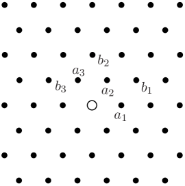
(a) Neighbor Set

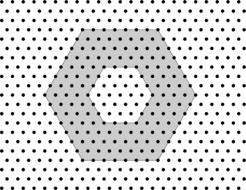
(b) Domain Decomposition

Figure 1. (a) The 12 neighboring bonds of each atom. (b) The atomistic region is $\Omega_{a}=\mathtt{Hex}(\epsilon R_{a})$. The blending region is $\Omega_{b}=\mathtt{Hex}(\epsilon R_{b})\setminus\Omega_{a}$. Here, $R_{a}=3$, $R_{b}=7$ and $K=4$.

3.2. The atomistic, continuum and blending regions

Let $\mathtt{Hex}(r)$ denote the closed hexagon centered at the origin, with sides aligned with the lattice directions $a_{1},a_{2},a_{3}$, and diameter $2r$.

For $R_{a}<R_{b}\in\mathbb{N}$, we define the atomistic, blending and continuum regions, respectively, as

$$\Omega_{a}:=\mathtt{Hex}(\epsilon R_{a}),\quad\Omega_{b}:=\mathtt{Hex}(\epsilon R_{b})\setminus\Omega_{a},\quad\text{and}\quad\Omega_{c}:={\rm clos}\left(\Omega\setminus\left(\Omega_{a}\cup\Omega_{b}\right)\right).$$

We denote the blending width by $K:=R_{b}-R_{a}$. Moreover, we define the corresponding lattice sites

$$\mathcal{L}^{a}:=\mathcal{L}\cap\Omega_{a},\qquad\mathcal{L}^{b}:=\mathcal{L}\cap\Omega_{b},\qquad\text{and}\qquad\mathcal{L}^{c}:=\mathcal{L}\cap\Omega_{c}.$$

For simplicity, we will again use $\mathcal{L}$ as the finite element nodes, that is, every atom is a repatom.

For a map $\mathbf{v}:\mathbb{L}\rightarrow\mathbb{R}^{2}$ and bond directions $r,s\in\mathcal{N}$, we define the finite difference operators

$$D_{r}v(x):=\frac{v(x+r)-v(x)}{\epsilon}\quad\text{and}\quad D_{r}D_{s}v(x):=\frac{D_{s}v(x+r)-D_{s}v(x)}{\epsilon}.$$

We define the space of all admissible displacements, $\mathcal{U}$, as all discrete functions $\mathbb{L}\rightarrow\mathbb{R}^{2}$ which are $\Omega$-periodic and satisfy the mean zero condition on the computational domain:

$$\mathcal{U}:=\Big{\{}\mathbf{u}:\mathbb{L}\rightarrow\mathbb{R}^{2}:\text{$u(x)$ is $\Omega$-periodic and }{\textstyle\sum_{x\in\mathcal{L}}}u(x)=0\Big{\}}.$$

For a given matrix $B\in\mathbb{R}^{2\times 2}$, $\mathrm{det}(B)>0$, we admit deformations $\mathbf{y}$ from the space

$$\mathcal{Y}_{B}:=\big{\{}\mathbf{y}:\mathbb{L}\rightarrow\mathbb{R}^{2}:y(x)=Bx+u(x),\,\forall x\in\mathbb{L}\,\text{for some $\mathbf{u}\in\mathcal{U}$}\big{\}}.$$

For a displacement $\mathbf{u}\in\mathcal{U}$ and its discrete directional derivatives, we employ the weighted discrete $\ell_{\epsilon}^{2}$ and $\ell_{\epsilon}^{\infty}$ norms given by

$$\|\mathbf{u}\|_{\ell_{\epsilon}^{2}}:=\left(\epsilon^{2}\sum_{x\in\mathcal{L}}|u(x)|^{2}\right)^{1/2},\quad\|\mathbf{u}\|_{\ell_{\epsilon}^{\infty}}:=\max\limits_{x\in\mathcal{L}}|u(x)|,\quad\text{and}$$

$$\qquad\quad\|D\mathbf{u}\|_{\ell_{\epsilon}^{2}}:=\left(\epsilon^{2}\sum_{x\in\mathcal{L}}\sum_{i=1}^{3}|D_{a_{i}}u(x)|^{2}\right)^{1/2}.$$

The inner product associated with $\ell^{2}_{\epsilon}$ is

$$\langle\mathbf{u},\mathbf{w}\rangle:=\epsilon^{2}\sum\limits_{x\in\mathcal{L}}u(x)\cdot w(x).$$

3.3. The B-QCF operator

The total scaled atomistic energy for a periodic computational cell $\Omega$ is

$$\mathcal{E}^{a}(\mathbf{y})= \frac{\epsilon^{2}}{2}\sum_{x\in\mathcal{L}}\sum_{r\in\mathcal{N}}\phi(D_{r}y({x}))={\epsilon^{2}}\sum_{x\in\mathcal{L}}\sum_{i=1}^{3}\big{[}\phi(D_{a_{i}}y({x}))+\phi(D_{b_{i}}y({x}))\big{]},$$ (3.1)

where $\phi\in C^{2}(\mathbb{R}^{2})$, for the sake of simplicity. Typically, one assumes $\phi(r)=\varphi(|r|)$; the more general form we use gives rise to a simplified notation; see also [30]. We define $\phi^{\prime}(r)\in\mathbb{R}^{2}$ and $\phi^{\prime\prime}(r)\in\mathbb{R}^{2\times 2}$ to be, respectively, the gradient and hessian of $\phi$.

The equilibrium equations are given by the force balance at each atom,

$$F^{a}(x;y)+f(x;y)=0,\quad\text{for}\quad x\in\mathcal{L},$$ (3.2)

where $f(x;y)$ are the external forces and $F^{a}(x;y)$ are the atomistic forces (per unit volume $\epsilon^{2}$)

$$F^{a}(x;y):= -\frac{1}{\epsilon^{2}}\frac{\partial\mathcal{E}^{a}(\mathbf{y})}{\partial y(x)}$$

$$= -\frac{1}{\epsilon}\sum_{i=1}^{3}\Big{[}\phi^{\prime}\left(D_{a_{i}}y(x)\right)+\phi^{\prime}\left(D_{-a_{i}}y(x)\right)\Big{]}-\frac{1}{\epsilon}\sum_{i=1}^{3}\Big{[}\phi^{\prime}\left(D_{b_{i}}y(x)\right)+\phi^{\prime}\left(D_{-b_{i}}y(x)\right)\Big{]}.$$

Again, since $\mathbf{u}=\mathbf{y}-\mathbf{y}_{B}$, where $y_{B}(x)=Bx$, is assumed to be small we can linearize the atomistic equilibrium equation (3.2) about $\mathbf{y}_{B}$:

$$\left(L^{a}\mathbf{u}^{a}\right)(x)=f(x),\quad\text{for}\quad x\in\mathcal{L},$$

where $\left(L^{a}\mathbf{v}\right)(x)$, for a displacement $\mathbf{v}$, is given by

$$\left(L^{a}\mathbf{v}\right)(x)=-\sum_{i=1}^{3}\phi^{\prime\prime}(Ba_{i})D_{a_{i}}D_{a_{i}}v(x-a_{i})-\sum_{i=1}^{3}\phi^{\prime\prime}(Bb_{i})D_{b_{i}}D_{b_{i}}v(x-b_{i}),\quad\text{for}\quad x\in\mathcal{L}.$$

The QCL approximation uses the Cauchy–Born extrapolation rule to approximate the nonlocal atomistic model by a local continuum model [39, 37, 25]. According to the bond density lemma [30, Lemma 3.2] (see also [36]), we can write the total QCL energy as a sum of the bond density integrals

$$\mathcal{E}^{c}(\mathbf{y})=\int_{\Omega}\sum_{r\in\mathcal{N}}\phi(\partial_{r}y)\,dx=\sum_{x\in\mathcal{L}}\sum_{r\in\mathcal{N}}\int_{0}^{1}\phi\big{(}\partial_{r}y(x+tr)\big{)}dt,$$ (3.3)

where $\partial_{r}y(x)=\frac{d}{dt}y(x+tr)|_{t=0}$ denotes the directional derivative. We compute the continuum force $F^{c}(x;y)=-\frac{1}{\epsilon^{2}}\frac{\partial\mathcal{E}^{c}}{\partial y(x)}$, and linearize the force equation about the uniform deformation $\mathbf{y}_{B}$ to obtain

$$\left(L^{c}\mathbf{u}^{c}\right)(x)=f(x),\quad\text{for}\quad x\in\mathcal{L}.$$

To formulate the B-QCF method, let the blending function $\beta(s):\mathbb{R}^{2}\rightarrow[0,1]$ be a ”smooth”, $\Omega$-periodic function. We shall suppose throughout that $R_{a},R_{b}$ are chosen in such a way that

$${\rm supp}(D_{a_{i_{1}}}D_{a_{i_{2}}}D_{a_{i_{3}}}\beta)\subset\Omega_{b}\qquad\forall i\in\{1,\dots,6\}^{3}.$$ (3.4)

Then, the (nonlinear) B-QCF forces are given by

$$F^{bqcf}(x;y):=\beta(x)F^{a}(x;y)+(1-\beta(x))F^{c}(x;y),$$

and linearizing the equilibrium equation $F^{bqcf}+f=0$ about $y_{B}$ yields

$$\begin{split}&(L^{bqcf}\mathbf{u}^{bqcf})(x)=f(x),\quad\text{for }x\in\mathcal{L},\\ &\text{where}\quad(L^{bqcf}\mathbf{v})(x)=\beta(x)(L^{a}\mathbf{v})(x)+(1-\beta(x))(L^{c}\mathbf{v})(x).\end{split}$$ (3.5)

Since the nearest neighbor terms in the atomistic and the QCL models are the same, we will focus on the second-neighbor interactions. We rewrite the operator $L^{bqcf}$ in the form

$$(L^{bqcf}\mathbf{v})(x)=~{} \sum_{r\in\mathcal{N}}(L^{bqcf}_{r}\mathbf{v})(x),$$

$$\text{where}\quad L^{bqcf}_{r}\mathbf{v}(x)=~{} \beta(x)(L^{a}_{r}\mathbf{v})(x)+(1-\beta(x))(L^{c}_{r}\mathbf{v})(x),$$

where the nearest-neighbor operators are given by

$$L^{a}_{a_{j}}\mathbf{v}(x)=L^{c}_{a_{j}}\mathbf{v}(x)=-\phi^{\prime\prime}(Ba_{j})D_{a_{j}}D_{a_{j}}v(x-a_{j}),$$

and the second-neighbor operators, stated for convenience only for $b_{1}=a_{1}+a_{2}$, by

$$\left(L^{a}_{b_{1}}\mathbf{u}\right)(x)= -\phi^{\prime\prime}(Bb_{1})D_{b_{1}}D_{b_{1}}v(x-b_{1}),\quad\text{while}$$

$$\left(L^{c}_{b_{1}}\mathbf{u}\right)(x)= -\phi^{\prime\prime}(Bb_{1})\big{[}D_{a_{1}}D_{a_{1}}u(x-a_{1})+D_{a_{2}}D_{a_{2}}u(x-a_{2})\big{.}$$

$$\qquad\qquad\qquad\big{.}+D_{a_{1}}D_{a_{2}}u(x-a_{1})+D_{a_{1}}D_{a_{2}}u(x-a_{2})\big{]}.$$

3.4. Auxiliary results

The following is the 2D counterpart of the summation by parts formula. The proof is straightforward.

Lemma 3.1 (Summation by parts).

For any $\mathbf{u}\in\mathcal{U}$ and any direction $r\in\mathbb{Z}^{2}$, we have

$$\sum_{x\in\mathcal{L}}D_{r}D_{r}u(x-r)\cdot u(x)=-\sum_{x\in\mathcal{L}}D_{r}u(x-r)\cdot D_{r}u(x-r).$$ (3.6)

The second auxiliary result we require is a trace- or Poincaré-type inequality to bound $\|\mathbf{u}\|_{\ell^{2}_{\epsilon}(\Omega_{b})}$ in terms of global norms. As a first step we establish a continuous version of the inequality we are seeking. The key technical ingredient in its proof is a sharp trace inequality, which is stated in Section 5.

Lemma 3.2.

Let $r_{a}<r_{b}\in(0,1/2]$, and let $H:={\tt Hex}(r_{b})\setminus{\tt Hex}(r_{a})$; then there exists a constant $C$ that is independent of $r_{a},r_{b}$ such that

$$\|u\|_{L^{2}(H)}^{2}\leq C\big{[}(r_{b}-r_{a})r_{b}|\log r_{b}|\big{]}\|\partial u\|_{L^{2}(\Omega)}^{2}\qquad\forall u\in H^{1}(\Omega),\int_{\Omega}udx=0.$$ (3.7)

Proof.

Let $\Sigma:=\partial{\tt Hex}(1)$, and let $dS$ denote the surface measure, then

$$\|u\|_{L^{2}(H)}^{2}=\int_{r=r_{a}}^{r_{b}}\int_{\Sigma}|u|^{2}dS\,dr.$$

Applying (5.1) with $r_{0}=r$ and $r_{1}=1$ to each surface integral, we obtain

$$\|u\|_{L^{2}(H)}^{2}\leq(r_{b}-r_{a})\big{(}C_{0}\|u\|_{L^{2}(\Omega)}^{2}+C_{1}\|\partial u\|_{L^{2}(\Omega)}^{2}\big{)},$$

where $C_{0}\leq 8r_{b}$ and $C_{1}=2r_{b}|\log r_{b}|$. An application of Poincaré’s inequality yields (3.7). ∎

In our analysis, we require a result as (3.7) for discrete norms. We establish this next, using straightforward norm-equivalence arguments.

Lemma 3.3.

Suppose that $R_{b}\leq N/2$, then

$$\|\mathbf{u}\|_{\ell^{2}_{\epsilon}(\mathcal{L}^{b})}^{2}\leq C\,(C_{P}^{a,b})^{2}\|D\mathbf{u}\|_{\ell^{2}_{\epsilon}}^{2}\qquad\forall\mathbf{u}\in\mathcal{U}.$$ (3.8)

where $C$ is a generic constant, and $C_{P}^{a,b}:=\big{[}(\epsilon K)(\epsilon R_{b})|\log(\epsilon R_{b})|\big{]}^{1/2}$.

Proof.

Recall the identification of $\mathbf{u}$ with its corresponding $P_{1}$-interpolant. Let $T\in\mathcal{T}$ with corners $x_{j}$, $j=1,2,3$, then

$$\int_{T}u\,dx=\frac{|T|}{3}\sum_{j=1}^{3}u(x_{j}),\quad\text{and hence}\quad\int_{\Omega}u\,dx=0\quad\forall\mathbf{u}\in\mathcal{U}.$$

Let $r_{a}:=\epsilon R_{a}$ and $r_{b}:=\epsilon R_{b}$, then $H$ defined in Lemma 3.2 is identical to $\Omega_{b}$. For any element $T\subset\Omega_{b}$ it is straightforward to show that

$$\|\mathbf{u}\|_{\ell^{2}_{\epsilon}(T)}\leq C\|u\|_{L^{2}(T)}.$$

This immediately implies

$$\|\mathbf{u}\|_{\ell^{2}_{\epsilon}(\mathcal{L}^{b})}\leq C\|u\|_{L^{2}(H)},$$ (3.9)

for a constant $C$ that is independent of $\epsilon$, $R_{a}$, $K$ and $\mathbf{u}$. Applying (3.7) yields

$$\|\mathbf{u}\|_{\ell^{2}_{\epsilon}(\mathcal{L}^{b})}^{2}\leq C\big{[}(r_{b}-r_{a})r_{b}|\log r_{b}|\big{]}\|\partial u\|_{L^{2}(\Omega)}^{2}.$$

Fix $T\in\mathcal{T}$ and let $x_{j}\in T$ such that $x_{j}+a_{j}\in T$ as well. Employing [30, Eq. (2.1)] we obtain

$$\sum_{j=1}^{3}\big{|}D_{a_{j}}u(x_{j})\big{|}^{2}=\sum_{j=1}^{3}\big{|}(\partial u|_{T})a_{j}\big{|}^{2}={\textstyle\frac{3}{2}}\big{|}\partial u|_{T}\big{|}^{2},$$

and summing over $T\in\mathcal{T},T\subset\bar{\Omega}$ we obtain that $\|\partial u\|_{L^{2}(\Omega)}\leq C\|D\mathbf{u}\|_{\ell^{2}_{\epsilon}}$. This concludes the proof. ∎

3.5. Bounds on $L^{bqcf}_{b_{1}}$

We focus only on the $b_{1}$-bonds, however, by symmetry analogous results hold for all second-neighbor bonds. As in the 1D case, we begin by converting the quadratic form $\langle L^{bqcf}_{b_{1}}\mathbf{u},\mathbf{u}\rangle$ into divergence form. To that end it is convenient to define the bond-dependent symmetric bilinear forms and quadratic forms (although we write them like a norm they are typically indefinite)

$$\langle r,s\rangle_{b}:=r^{\rm T}\phi^{\prime\prime}(Bb)s,\quad\text{and}\quad|r|_{b}^{2}:=\langle r,r\rangle_{b},\qquad\text{for }r,s,b\in\mathbb{R}^{2}.$$

Lemma 3.4.

For any displacement $\mathbf{u}\in\mathcal{U}$, we have

$$\langle L^{bqcf}_{b_{1}}\mathbf{u},\mathbf{u}\rangle=\langle L^{c}_{b_{1}}\mathbf{u},\mathbf{u}\rangle-\epsilon^{4}\sum_{x\in\mathcal{L}}\beta(x-a_{2})|D_{a_{1}}D_{a_{2}}u(x-a_{1}-a_{2})|_{b_{1}}^{2}+\mathbf{R}_{b_{1}}+\mathbf{S}_{b_{1}},$$ (3.10)

where

$$\begin{split}\mathbf{R}_{b_{1}}:=&-\epsilon^{4}\sum_{x\in\mathcal{L}}\big{\{}D_{a_{1}}\beta(x-2a_{1})\big{\langle}D_{a_{1}}u(x-2a_{1}),D_{a_{2}}D_{a_{2}}u(x-a_{1}-a_{2})\big{\rangle}_{b_{1}}\\ &\qquad\qquad\quad+D_{a_{2}}\beta(x-a_{2})\big{\langle}D_{a_{1}}u(x-a_{1}),D_{a_{1}}D_{a_{2}}u(x-a_{1}-a_{2})\big{\rangle}_{b_{1}}\big{\}},\quad\text{and}\\ \mathbf{S}_{b_{1}}:=&-\epsilon^{4}\sum_{x\in\mathcal{L}}D_{a_{1}}D_{a_{1}}\beta(x-2a_{1})\big{\langle}u(x-a_{1}),D_{a_{2}}D_{a_{2}}u(x-a_{1}-a_{2})\big{\rangle}_{b_{1}}.\end{split}$$ (3.11)

Proof.

For this purely algebraic proof we may assume without loss of generality that $\phi^{\prime\prime}(Bb_{1})={\rm I}$. In general, one may simply replace all Euclidean inner products with $\langle\cdot,\cdot\rangle_{b_{1}}$.

Starting from (3.5), we have

$$\langle L^{bqcf}_{b_{1}}\mathbf{u},\mathbf{u}\rangle= \langle L^{c}_{b_{1}}\mathbf{u},\mathbf{u}\rangle+\langle L^{a}_{b_{1}}\mathbf{u}-L^{c}_{b_{1}}\mathbf{u},\beta\mathbf{u}\rangle$$

$$= \langle L^{c}_{b_{1}}\mathbf{u},\mathbf{u}\rangle-\epsilon^{2}\sum_{x\in\mathcal{L}}\beta(x)u(x)\cdot\left[D_{b_{1}}D_{b_{1}}u(x-b_{1})-D_{a_{1}}D_{a_{1}}u(x-a_{1})\right.$$

$$\qquad\qquad\left.-D_{a_{2}}D_{a_{2}}u(x-a_{2})-D_{a_{1}}D_{a_{2}}u(x-a_{1})-D_{a_{1}}D_{a_{2}}u(x-a_{2})\right].$$

We will focus our analysis on $\langle L^{a}_{b_{1}}\mathbf{u}-L^{c}_{b_{1}}\mathbf{u},\beta\mathbf{u}\rangle$.

Noting that $b_{1}=a_{1}+a_{2}$, one can recast $D_{b_{1}}D_{b_{1}}u(x-b_{1})$ as

$$D_{b_{1}} D_{b_{1}}u(x-b_{1})$$

$$= \frac{1}{\epsilon^{2}}\left[u(x+b_{1})-2u(x)+u(x-b_{1})\right]$$

$$= D_{a_{1}}D_{a_{2}}u(x)+D_{a_{1}}D_{a_{1}}u(x-a_{1})+D_{a_{2}}D_{a_{2}}u(x-a_{2})+D_{a_{1}}D_{a_{2}}u(x-a_{1}-a_{2}).$$

Applying the summation by parts formula (3.6) to $\langle L^{a}_{b_{1}}\mathbf{u}-L^{c}_{b_{1}}\mathbf{u},\beta\mathbf{u}\rangle$, we get

$$\langle L^{a}_{b_{1}}\mathbf{u}-L^{c}_{b_{1}}\mathbf{u},\beta\mathbf{u}\rangle= -\epsilon^{3}\sum_{x\in\mathcal{L}}\beta(x)u(x)\cdot\Big{[}D_{a_{1}}D_{a_{1}}D_{a_{2}}u(x-a_{1})-D_{a_{1}}D_{a_{1}}D_{a_{2}}u(x-a_{1}-a_{2})\Big{]}$$

$$= -\epsilon^{4}\sum_{x\in\mathcal{L}}\beta(x)u(x)\cdot D_{a_{1}}D_{a_{1}}D_{a_{2}}D_{a_{2}}u(x-a_{1}-a_{2})$$

$$= \epsilon^{4}\sum_{x\in\mathcal{L}}D_{a_{1}}D_{a_{2}}D_{a_{2}}u(x-a_{1}-a_{2})\cdot D_{a_{1}}\Big{(}\beta(x-a_{1})u(x-a_{1})\Big{)}$$

$$= \epsilon^{4}\sum_{x\in\mathcal{L}}D_{a_{1}}D_{a_{2}}D_{a_{2}}u(x-a_{1}-a_{2})\cdot\Big{[}\beta(x)D_{a_{1}}u(x-a_{1})+u(x-a_{1})D_{a_{1}}\beta(x-a_{1})\Big{]}.$$

Another application of the summation by parts formula (3.6) converts $\langle L^{a}_{b_{1}}\mathbf{u}-L^{c}_{b_{1}}\mathbf{u},\beta\mathbf{u}\rangle$ into

$$\langle L^{a}_{b_{1}}\mathbf{u}-L^{c}_{b_{1}}\mathbf{u},\beta\mathbf{u}\rangle= \epsilon^{4}\sum_{x\in\mathcal{L}}D_{a_{1}}D_{a_{2}}D_{a_{2}}u(x-a_{1}-a_{2})\cdot\big{(}u(x-a_{1})D_{a_{1}}\beta(x-a_{1})\big{)}$$

$$\quad-\epsilon^{4}\sum_{x\in\mathcal{L}}D_{a_{1}}D_{a_{2}}u(x-a_{1}-a_{2})\cdot\big{(}D_{a_{2}}\beta(x-a_{2})D_{a_{1}}u(x-a_{1})\big{)}$$

$$\quad\quad-\epsilon^{4}\sum_{x\in\mathcal{L}}D_{a_{1}}D_{a_{2}}u(x-a_{1}-a_{2})\cdot\big{(}\beta(x-a_{2})D_{a_{1}}D_{a_{2}}u(x-a_{1}-a_{2})\big{)}.$$

The first two terms on the right-hand side can be rewritten as

$$\epsilon^{4} \sum_{x\in\mathcal{L}}\big{\{}D_{a_{1}}D_{a_{2}}D_{a_{2}}u(x-a_{1}-a_{2})\cdot\big{(}u(x-a_{1})D_{a_{1}}\beta(x-a_{1})\big{)}\big{.}$$

$$\qquad\Big{.}-D_{a_{1}}D_{a_{2}}u(x-a_{1}-a_{2})\cdot\big{(}D_{a_{2}}\beta(x-a_{2})D_{a_{1}}u(x-a_{1})\big{)}\big{\}}$$

$$=-\epsilon^{4}\sum_{x\in\mathcal{L}}\Big{(}u(x-a_{1})D_{a_{1}}D_{a_{1}}\beta(x-2a_{1})\Big{)}\cdot D_{a_{2}}D_{a_{2}}u(x-a_{1}-a_{2})$$

$$\qquad-\epsilon^{4}\sum_{x\in\mathcal{L}}\big{\{}D_{a_{1}}\beta(x-2a_{1})D_{a_{1}}u(x-2a_{1})\cdot D_{a_{2}}D_{a_{2}}u(x-a_{1}-a_{2})\big{.}$$

$$\qquad\qquad\qquad\big{.}+D_{a_{2}}\beta(x-a_{2})D_{a_{1}}u(x-a_{1})\cdot D_{a_{1}}D_{a_{2}}u(x-a_{1}-a_{2})\big{\}}$$

$$=\mathbf{S}_{b_{1}}+\mathbf{R}_{b_{1}}.$$

Thus, we obtain (3.10) and (3.11). ∎

Next, we will bound the singular terms $\mathbf{R}_{b_{1}}$ and $\mathbf{S}_{b_{1}}$, for which we introduce the notation

$$\|D^{(2)}\beta\|_{\ell^{\infty}_{\epsilon}}:=\max_{1\leq i,j\leq 6}\|D_{a_{i}}D_{a_{j}}\beta\|_{\ell^{\infty}_{\epsilon}},\quad\text{and}\quad\|D^{(3)}\beta\|_{\ell^{\infty}_{\epsilon}}:=\max_{1\leq i,j,k\leq 6}\|D_{a_{i}}D_{a_{j}}D_{a_{k}}\beta\|_{\ell^{\infty}_{\epsilon}}.$$

Lemma 3.5.

The terms $\mathbf{R}_{b_{1}}$ and $\mathbf{S}_{b_{1}}$ defined in (3.11) are bounded by

$$\left|\mathbf{R}_{b_{1}}\right|\leq 4\epsilon^{2}|\phi^{\prime\prime}(Bb_{1})|\,\|D\beta\|_{\ell_{\epsilon}^{\infty}}\|D\mathbf{u}\|_{\ell_{\epsilon}^{2}}^{2},\quad\text{and}$$ (3.12)

$$\left|\mathbf{S}_{b_{1}}\right|\leq C\epsilon^{2}|\phi^{\prime\prime}(Bb_{1})|\Big{[}\|D^{(2)}\beta\|_{\ell_{\epsilon}^{\infty}}+\|D^{(3)}\beta\|_{\ell_{\epsilon}^{\infty}}\,C_{P}^{a,b}\Big{]}\|D\mathbf{u}\|_{\ell_{\epsilon}^{2}}^{2},$$ (3.13)

where $C$ is a generic constant and $C_{P}^{a,b}$ is defined in Lemma 3.8.

Proof.

According to the expression of $\mathbf{R}_{b_{1}}$ given in (3.11) and noting that

$$\|D_{a_{2}}D_{a_{2}}\mathbf{u}\|_{\ell_{\epsilon}^{2}}^{2}\leq\frac{4}{\epsilon^{2}}\|D\mathbf{u}\|_{\ell_{\epsilon}^{2}}^{2}\quad\text{and}\quad\|D_{a_{1}}D_{a_{2}}\mathbf{u}\|_{\ell_{\epsilon}^{2}}^{2}\leq\frac{4}{\epsilon^{2}}\|D\mathbf{u}\|_{\ell_{\epsilon}^{2}}^{2},$$

we immediately obtain the first inequality of (3.12).

We first rewrite $\mathbf{S}_{b_{1}}$ as

$$\mathbf{S}_{b_{1}}= -\epsilon^{4}\sum_{x\in\mathcal{L}}D_{a_{1}}D_{a_{1}}\beta(x-2a_{1})\big{\langle}D_{a_{2}}D_{a_{2}}u(x-a_{1}-a_{2}),u(x-a_{1})\big{\rangle}_{b_{1}}$$

$$= -\epsilon^{4}\sum_{x\in\mathcal{L}}D_{a_{1}}D_{a_{1}}\beta(x-2a_{1})D_{a_{2}}\big{\langle}D_{a_{2}}u(x-a_{1}-a_{2}),u(x-a_{1}-a_{2})\big{\rangle}_{b_{1}}$$

$$\qquad+\epsilon^{4}\sum_{x\in\mathcal{L}}D_{a_{1}}D_{a_{1}}\beta(x-2a_{1})\big{\langle}D_{a_{2}}u(x-a_{1}-a_{2}),D_{a_{2}}u(x-a_{1}-a_{2})\big{\rangle}_{b_{1}}$$

$$= \epsilon^{4}\sum_{x\in\mathcal{L}}D_{a_{2}}D_{a_{1}}D_{a_{1}}\beta(x-2a_{1}-a_{2})\big{\langle}D_{a_{2}}u(x-a_{1}-a_{2})\cdot u(x-a_{1}-a_{2})\big{\rangle}_{b_{1}}$$

$$\qquad+\epsilon^{4}\sum_{x\in\mathcal{L}}D_{a_{1}}D_{a_{1}}\beta(x-2a_{1})\big{|}D_{a_{2}}u(x-a_{1}-a_{2})\big{|}_{b_{1}}^{2}.$$ (3.14)

For the second term in (3.14), we have

$$\Big{|}\epsilon^{4}\sum_{x\in\mathcal{L}}D_{a_{1}}D_{a_{1}}\beta(x-2a_{1})\big{|}D_{a_{2}}u(x-a_{1}-a_{2})\big{|}_{b_{1}}^{2}\Big{|}\leq\epsilon^{2}|\phi^{\prime\prime}(Bb_{1})|\|D^{(2)}\beta\|_{\ell_{\epsilon}^{\infty}}\|D\mathbf{u}\|_{\ell_{\epsilon}^{2}}^{2}.$$

For the first term, we have

$$\Big{|}\epsilon^{4}\sum_{x\in\mathcal{L}}D_{a_{2}}D_{a_{1}}D_{a_{1}}\beta(x-2a_{1}-a_{2})\big{\langle}D_{a_{2}}u(x-a_{1}-a_{2}),u(x-a_{1}-a_{2})\big{\rangle}_{b_{1}}\Big{|}$$

$$\qquad\leq\epsilon^{2}\,|\phi^{\prime\prime}(Bb_{1})|\,\|\mathbf{u}\,D_{a_{2}}D_{a_{1}}D_{a_{1}}\beta\|_{\ell_{\epsilon}^{2}}\|D\mathbf{u}\|_{\ell_{\epsilon}^{2}}\leq\epsilon^{2}\,|\phi^{\prime\prime}(Bb_{1})|\,\|D^{(3)}\beta\|_{\ell_{\epsilon}^{\infty}}\,\|\mathbf{u}\|_{\ell_{\epsilon}^{2}(\mathcal{L}^{b})}\,\|D\mathbf{u}\|_{\ell_{\epsilon}^{2}}.$$

The last inequality comes from the assumption (3.4), which ensures that ${\rm supp}(D_{a_{2}}D_{a_{1}}D_{a_{1}}\beta)\subset\Omega_{b}$.

Applying Lemma 3.3 yields the bound for ${\bf S}_{b_{1}}$. ∎

To summarize the estimates of this section we define a self-adjoint operator $\tilde{L}$ by

$$\langle\tilde{L}\mathbf{u},\mathbf{u}\rangle:=\langle L^{c}\mathbf{u},\mathbf{u}\rangle-\epsilon^{4}\sum_{j=1}^{3}\sum_{x\in\mathcal{L}}\beta(x-a_{2})\big{|}D_{a_{j}}D_{a_{j+1}}u(x-a_{1}-a_{2})\big{|}_{b_{1}}^{2};$$ (3.15)

then, Lemma 3.4 and Lemma 3.5 immediately yield the following result.

Corollary 3.1.

Suppose that $R_{a}$ and $R_{b}$ are defined such that (3.4) holds; then, for all $\mathbf{u}\in\mathcal{U}$,

$$\langle L^{bqcf}\mathbf{u},\mathbf{u}\rangle\geq\langle\tilde{L}\mathbf{u},\mathbf{u}\rangle-C\,C^{\prime\prime}\big{[}\epsilon^{2}\|D\beta\|_{\ell^{\infty}}+\epsilon^{2}\|D^{(2)}\beta\|_{\ell^{\infty}}+\epsilon^{2}C_{P}^{a,b}\|D^{(3)}\beta\|_{\ell^{\infty}}\big{]}\|D\mathbf{u}\|_{\ell^{2}_{\epsilon}}^{2},$$ (3.16)

where $C$ is a generic constant, $C^{\prime\prime}:=\max_{j=1,2,3}|\phi^{\prime\prime}(Bb_{j})|$ and $C_{P}^{a,b}$ is defined in Lemma 3.8.

Based on the analysis and numerical experiments in [30] for a similar linearized operator we expect that the region of stability for $\tilde{L}$ is the same as for $L^{a}$; that is, $\tilde{L}$ is positive definite for a macroscopic strain $B$ if and only if $L^{a}$ is positive definite. However, we are at this point unable to prove this result. Instead, we have the following weaker result. The proof is elementary.

Proposition 3.1.

Suppose that $B\in\mathbb{R}^{2\times 2}$ is such that $L^{c}$ is positive definite,

$$\langle L^{c}\mathbf{u},\mathbf{u}\rangle\geq\gamma_{c}\|D\mathbf{u}\|_{\ell^{2}_{\epsilon}}^{2}\qquad\forall\mathbf{u}\in\mathcal{U},$$

and suppose that $\phi^{\prime\prime}(Bb_{j})\leq\delta{\rm I}$ where $\delta<\gamma_{c}/4$, then $\tilde{L}$ is positive definite,

$$\langle\tilde{L}\mathbf{u},\mathbf{u}\rangle\geq\tilde{\gamma}\|D\mathbf{u}\|_{\ell^{2}_{\epsilon}}^{2}\qquad\forall\mathbf{u}\in\mathcal{U},$$ (3.17)

with $\tilde{\gamma}=\gamma_{c}-4\delta$.

3.6. Positivity of the B-QCF operator in 2D

The blending width $K$ is again a crucial ingredient in the stability analysis for $L^{bqcf}$. Due to the simple geometry we have chosen it straightforward to generalize Lemma 2.5 to the two-dimensional case, using the same arguments as in 1D.

Lemma 3.6.

It is possible to choose $\beta$ such that

$$\|D^{(j)}\beta\|_{\ell^{\infty}}\leq C_{\beta}(K\epsilon)^{-j}.\quad\text{for }j=1,2,3,$$ (3.18)

Since we cannot fully characterize the stability of $\tilde{L}$ in terms of the stability of $L^{a}$ or $L^{c}$ we will only prove stability of $L^{bqcf}$ subject to the assumption that $\tilde{L}$ is stable. Proposition 3.1 gives sufficient conditions.

Theorem 3.1.

Suppose that $\beta$ is chosen quasi-optimally so that (3.18) is attained; then,

$$\langle L^{bqcf}\mathbf{u},\mathbf{u}\rangle\geq\gamma_{bqcf}\|D\mathbf{u}\|_{\ell^{2}_{\epsilon}}^{2},$$

where

$$\gamma_{bqcf}:=\tilde{\gamma}-C\,C^{\prime\prime}\,\big{[}\epsilon^{-1/2}K^{-5/2}|\epsilon R_{b}\log(\epsilon R_{b})|^{1/2}\big{]},$$

where $C$ is a generic constant and $C^{\prime\prime}$ is defined in Corollary 3.1.

In particular, if $\tilde{L}$ is positive definite (3.17) and if $K$ is sufficiently large, then $L^{bqcf}$ is positive definite.

Proof.

From Corollary 3.1 and (3.18) we obtain

$$\langle L^{bqcf}\mathbf{u},\mathbf{u}\rangle\geq~{} \big{\{}\tilde{\gamma}-C\,C^{\prime\prime}\,\big{[}\epsilon^{2}(\epsilon K)^{-1}+\epsilon^{2}(\epsilon K)^{-2}+\epsilon^{2}(\epsilon K)^{-5/2}|\epsilon R_{b}\log(\epsilon R_{b})|^{1/2}\big{]}\big{\}}\|D\mathbf{u}\|_{\ell^{2}_{\epsilon}}^{2}$$

$$\geq~{} \big{\{}\tilde{\gamma}-C\,C^{\prime\prime}\,\big{[}\epsilon^{-1/2}K^{-5/2}|\epsilon R_{b}\log(\epsilon R_{b})|^{1/2}\big{]}\big{\}}\|D\mathbf{u}\|_{\ell^{2}_{\epsilon}}^{2}.\qed$$

Remark 3.1.

Suppose that $\tilde{\gamma}>0$, uniformly as $N\to\infty$ (or, $\epsilon\to 0$). In this limit, we would like to understand how to optimally scale $K$ with $R_{a}$. (Note that $R_{a}$ controls the modeling error; cf. Remark 3.3.) We consider three different scalings of $R_{a}$.

Case 1: Suppose that $R_{a}$ is bounded as $\epsilon\to 0$. In that case, we obtain

$$\gamma_{bqcf}-\tilde{\gamma}=~{} -C\,C^{\prime\prime}\,\epsilon^{-1/2}K^{-5/2}|\epsilon(R_{a}+K)\log(\epsilon(R_{a}+K))|^{1/2}$$

$$=~{} -C\,C^{\prime\prime}\,K^{-2}\big{|}\big{(}1+{\textstyle\frac{R_{a}}{K}}\big{)}\big{(}\log(\epsilon K)+\log(1+{\textstyle\frac{R_{a}}{K}})\big{)}\big{|}^{1/2}$$

$$\eqsim~{} -C\,C^{\prime\prime}\,K^{-2}|\log(\epsilon K)|^{1/2}.$$ (3.19)

From this it is easy to see that $L^{bqcf}$ will be positive definite provided we select $K\gg|\log\epsilon|^{1/4}$.

Case 2: Suppose that $1\ll R_{a}\ll\epsilon^{-1}$; to precise, let $R_{a}\sim\epsilon^{-\alpha}$ for some $\alpha\in(0,1)$. Then, a similar computation as (3.19) yields

$$\gamma_{bqcf}-\tilde{\gamma}\eqsim K^{-5/2}\big{|}(K+\epsilon^{-\alpha})(\log\epsilon+\log(K+\epsilon^{-\alpha}))\big{|}^{1/2},$$

and we deduce that, in this case, $L^{bqcf}$ will positive definite provided we select $K\gg\epsilon^{-\alpha/5}|\log\epsilon|^{1/5}$.

Case 3: Finally, the case when the atomistic region is macroscopic, i.e., $R_{a}=O(\epsilon^{-1})$, can be treated precisely as the 1D case and hence we obtain that, if we select $K\gg\epsilon^{-1/5}$, then $L^{bqcf}$ is positive.

In summary, we have shown that, in the limit as $\epsilon\to 0$, if $\tilde{L}$ is positive definite, $R_{a}=O(\epsilon^{-\alpha})$ and if we choose

$$K\gg\begin{cases}|\log{\epsilon}|^{1/4},&\quad\alpha=0,\\ |\log\epsilon|^{1/5}\epsilon^{-\alpha/5},&\quad 0<\alpha<1,\\ \epsilon^{-1/5},&\quad\alpha=1,\end{cases}$$ (3.20)

then the B-QCF operator $L^{bqcf}$ is positive definite and $\gamma^{bqcf}\sim\tilde{\gamma}$ as $\epsilon\to 0$. We emphasize that these are very mild restrictions on the blending width. ∎

It remains to show that the sufficient conditions we derived to guarantee positivity of $L^{bqcf}$ are sharp. A result as general as (2.13) in 1D would be very technical to obtain; instead, we offer a brief formal discussion for a special case.

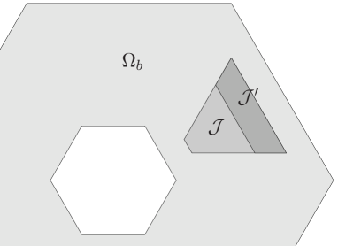
Figure 2. Visualization of the construction discussed in 3.2: the white region is the atomistic domain, the light gray region the blending region, the medium gray region and dark gray regions together are the set $\mathcal{J}$ and the dark gray region is the set $\mathcal{J}^{\prime}$.

Remark 3.2.

We consider again the limit as $\epsilon\to 0$, and for simplicity restrict ourselves to the case where $0\ll K\eqsim\epsilon^{-\theta}$ and $0\ll R_{a}\eqsim\epsilon^{-\alpha}$, for $0<\theta\leq\alpha\leq 1$. In particular, $R_{b}\eqsim\epsilon^{-\alpha}$ as well.

We assume that $D_{a_{3}}\beta(x)=0$ for all $x\in\mathcal{J}\subset\mathcal{L}^{b}$, as depicted in Figure 2. The set $\mathcal{J}$ should be chosen so that its size is comparable with that of $\mathcal{L}^{b}$, but sufficiently small to still allow $\beta$ to satisfy the bound (3.18). We can now repeat the 1D argument along atomic layers to obtain that

$$D_{a_{2}}D_{a_{1}}D_{a_{1}}\beta(x)\leq-{\textstyle\frac{1}{2}}(\epsilon K)^{-3}\eqsim-\epsilon^{-3+3\theta}$$

for all $x$ in a subset $\mathcal{J}^{\prime}\subset\mathcal{J}$ containing entire atomic planes, that has comparable size to $\mathcal{J}$; that is, $\#\mathcal{J}^{\prime}\eqsim KR_{b}\eqsim\epsilon^{-\theta-\alpha}$.

Suppose now that $\phi^{\prime\prime}(Bb_{1})$ has a negative eigenvalue $\lambda$ with corresponding normalized eigenvector $\hat{u}\in\mathbb{R}^{2}$, then we seek test functions of the form $u(x)=\mu(x)\hat{u}$. It is now relatively straightforward, applying the 1D argument in normal direction and using a smooth cut-off in the tangential direction, to construct $\mu$ supported in $\mathcal{J}^{\prime}$ with $D_{a_{2}}\mu(x)\eqsim(\epsilon^{2}\#\mathcal{J}^{\prime})^{-1/2}$ so that $\|D\mathbf{u}\|_{\ell^{2}_{\epsilon}}\eqsim 1$, and

$$\epsilon^{4}\sum_{x\in\mathcal{L}}D_{a_{2}}D_{a_{1}}D_{a_{1}}\beta(x-2a_{1}-a_{2})\big{\langle}D_{a_{2}}u(x-a_{1}-a_{2}),u(x-a_{1}-a_{2})\big{\rangle}_{b_{1}}$$

$$\hskip 28.45274pt=\epsilon^{4}\lambda_{1}\sum_{x\in\mathcal{L}}D_{a_{2}}D_{a_{1}}D_{a_{1}}\beta(x-2a_{1}-a_{2})D_{a_{2}}\mu(x-a_{1}-a_{2})\mu(x-a_{1}-a_{2})$$

$$\hskip 28.45274pt\lesssim-\epsilon^{4}\lambda_{1}(\#\mathcal{J}^{\prime})(K\epsilon)^{-3}(\epsilon^{2}\#\mathcal{J}^{\prime})^{-1/2}\eqsim-\epsilon^{(5\theta-\alpha)/2}.$$

This shows that, if $K\ll\epsilon^{-\alpha/5}$, then $L^{bqcf}$ is necessarily indefinite.

In summary, for the specific interface geometry and a particular choice of $\beta$ (which does, however, lead to the quasi-optimal bound (3.18)) we have shown that Theorem 3.1 is sharp up to logarithmic terms. ∎

Remark 3.3.

In practise, for the computation of different types of defects, we would first choose an appropriate scaling $R_{a}=\epsilon^{-\alpha}$ for the atomistic region, considering the accuracy of the B-QCF method, and then choose the blending width $K$ in order to ensure stability.

For instance, for a point defect in 2D with zero Burger’s vector it is expected that the displacement field satisfies $u_{a}(x)=y_{a}(x)-Bx\eqsim\epsilon/r$, where $r$ is the distance from the defect [33, 30]. Without coarse-graining, the local continuum (QCL) model has a modeling error of order $O(\epsilon^{2}|\partial^{3}u_{a}|)$ (see [29, 20, 10] for proofs in 1D and [40] for a proof in arbitrary dimensions); and although we have not established it rigorously, we expect that modeling error for the B-QCF method outside the atomistic region is also of second order; see also [13].

From $u(x)\eqsim\epsilon/r$ we can make the reasonable assumption that $|\partial^{3}y_{a}|\eqsim\epsilon/r^{4}$, from which we obtain (assuming also stability) that the total error is of the order

$$\|\partial(y_{a}-y_{bqcf})\|_{L^{2}}\eqsim\epsilon^{2}\|\partial^{3}y_{a}\|_{L^{2}(\Omega\setminus\Omega_{a})}\eqsim\epsilon^{3}\Big{(}\int_{\epsilon R_{a}}^{1}r|r^{-4}|^{2}dr\Big{)}^{1/2}\eqsim R_{a}^{-3}.$$

Hence, if we wish to obtain $\|\partial(y_{a}-y_{bqcf})\|_{L^{2}}\eqsim\epsilon^{k}$, $0<k<3$, then we need to choose

$$R_{a}\eqsim\epsilon^{-k/3},\quad\text{and consequently}\quad K\gg\epsilon^{-k/15}|\log\epsilon|^{1/5}.$$

With this choice we can ensure both the stability and $O(\epsilon^{k})$ accuracy of the B-QCF method; provided that our assumption that the B-QCF method has indeed a second-order modelling error is correct. ∎

4. Conclusion

We have studied the stability a blended force-based quasicontinuum (B-QCF) method. In 1D we were able to identify an asymptotically optimal condition on the width of the blending region to ensure that the linearized B-QCF operator is coercive if and only if the atomistic operator is coercive as well. In the $2$D B-QCF model, we have obtained rigorous sufficient conditions and have presented a heuristic argument suggesting that they are sharp up to logarithmic terms. In 2D our proof of coercivity of $L^{bqcf}$ relies on the coercivity of the auxiliary operator $\tilde{L}$ defined in (3.15), for which we cannot give sharp conditions at this point.

The main conclusion of this work is that the required blending width to ensure coercivity of the linearized B-QCF operator is surprisingly small.

Our analysis in this paper is the first step towards a complete a priori error analysis of the B-QCF method, which will require a coercivity analysis of the B-QCF operator linearized about arbitrary states, as well as a consistency analysis in negative Sobolev norms.

5. Appendix: A Trace Inequality

In the following trace theorem, $S(1)$ denotes the unit sphere in $\mathbb{R}^{d}$, $r:=|x|$ and $\theta:=x/|x|$. Upon taking $\psi\equiv 1$ and employing standard orthogonal decompositions it is easy to check that the result is sharp. In particular, for $d=2$, consider the case $u(x)=\log|x|$.

Lemma 5.1.

Let $d\geq 2$, $\psi:S(1)\to(0,1]$ be Lipschitz continuous, and $\Sigma:=\{\psi(\sigma)\sigma:\sigma\in S(1)\}$. Moreover, let $0<r_{0}<r_{1}\leq 1$, and $A:=\bigcup_{r_{0}<r<r_{1}}(r\Sigma)$, then

$$\|u\|_{L^{2}(r_{0}\Sigma)}^{2}\leq C_{0}\|u\|_{L^{2}(A)}^{2}+C_{1}\|\partial u\|_{L^{2}(A)}^{2},\quad\forall u\in H^{1}(A),$$ (5.1)

$$\text{where}\quad C_{0}=\frac{2d}{r_{1}-r_{0}}\Big{(}\frac{r_{0}}{r_{1}}\Big{)}^{d-1},\quad\text{and}\quad C_{1}=\begin{cases}2r_{0}|\log r_{0}|,&d=2\\ 2r_{0}/(d-2),&d\geq 3.\end{cases}$$ (5.2)

Proof.

Since $A$ is a Lipschitz domain we may assume, without loss of generality that $u\in C^{1}(\bar{A})$. The symbol $dS$ denotes the $(d-1)$-dimensional Hausdorff measure in $\mathbb{R}^{d}$.

Let $r_{0}<s<r_{1}$, then

$$\int_{r_{0}\Sigma}|u|^{2}dS=~{} r_{0}^{d-1}\int_{\Sigma}|u(r_{0}\sigma)|^{2}dS_{\sigma}$$

$$=~{} r_{0}^{d-1}\int_{\Sigma}\bigg{|}u(s\sigma)-\int_{r=r_{0}}^{s}\frac{d}{dr}u(r\sigma)dr\bigg{|}^{2}dS_{\sigma}$$

$$\leq~{} 2r_{0}^{d-1}\int_{\Sigma}\big{|}u(s\sigma)\big{|}^{2}dS_{\sigma}+2r_{0}^{d-1}\int_{\Sigma}\bigg{|}\int_{r=r_{0}}^{s}\partial u\cdot\sigma dr\bigg{|}^{2}dS_{\sigma}.$$ (5.3)

By hypothesis we have $|\sigma|\leq 1$ for all $\sigma\in\Sigma$, hence the second term on the right-hand side can be further estimated, applying also the Cauchy–Schwartz inequality, by

$$2r_{0}^{d-1}\int_{\Sigma}\bigg{|}\int_{r=r_{0}}^{s}\partial u\cdot\sigma dr\bigg{|}^{2}dS_{\sigma}\leq~{} 2r_{0}^{d-1}\int_{\Sigma}\int_{r=r_{0}}^{s}r^{-d+1}dr\,\int_{r=r_{0}}^{s}r^{d-1}|\partial u(r\sigma)|^{2}dr\,dS_{\sigma}$$

$$=~{} 2r_{0}^{d-1}(J(s)-J(r_{0}))\int_{r=r_{0}}^{s}\int_{r\Sigma}|\partial u|^{2}dS\,dr$$

$$\leq~{} 2r_{0}^{d-1}(J(s)-J(r_{0}))\|\partial u\|_{L^{2}(A)}^{2},$$

where $J^{\prime}(t)=t^{-d+1}$, that is, $J(t)=\log t$ if $d=2$ and $J(t)=t^{-d+2}/(-d+2)$ if $d\geq 3$. Since $J(s)$ is negative and strictly increasing for $s\leq 1$ we obtain

$$2r_{0}^{d-1}\int_{\Sigma}\bigg{|}\int_{r=r_{0}}^{s}\partial u\cdot\sigma dr\bigg{|}^{2}dS_{\sigma}\leq 2r_{0}^{d-1}|J(r_{0})|\|\partial u\|_{L^{2}(A)}^{2}.$$ (5.4)

Inserting (5.4) into (5.3), multiplying the resulting inequality by $s^{d-1}$ and integrating over $s\in(r_{0},r_{1})$ yields

$${\textstyle\frac{r_{1}^{d}-r_{0}^{d}}{d}}\|u\|_{L^{2}(r_{0}\Sigma)}^{2}=~{} \int_{s=r_{0}}^{r_{1}}s^{d-1}\int_{r_{0}\Sigma}|u|^{2}dS\,ds$$

$$\leq~{} 2r_{0}^{d-1}\int_{s=r_{0}}^{r_{1}}s^{d-1}\int_{\Sigma}\big{|}u(s\sigma)\big{|}^{2}dS_{\sigma}\,ds+2r_{0}^{d-1}J(r_{0}){\textstyle\frac{r_{1}^{d}-r_{0}^{d}}{d}}\|\partial u\|_{L^{2}(A)}^{2}.$$

Dividing through by $\frac{r_{1}^{d}-r_{0}^{d}}{d}$ we obtain

$$\|u\|_{L^{2}(r_{0}\Sigma)}^{2}\leq{\textstyle\frac{2dr_{0}^{d-1}}{r_{1}^{d}-r_{0}^{d}}}\|u\|_{L^{2}(A)}^{2}+2r_{0}^{d-1}J(r_{0})\|\partial u\|_{L^{2}(A)}^{2}.$$

Finally, estimating $r_{0}^{d}-r_{1}^{d}\geq(r_{1}-r_{0})r_{1}^{d-1}$ yields the stated trace inequality. ∎

6. Acknowledgments

We appreciate helpful discussions with Brian Van Koten.

References

• [1] S. Badia, P. Bochev, R. Lehoucq, M. L. Parks, J. Fish, M. Nuggehally, and M. Gunzburger. A force-based blending model for atomistic-to-continuum coupling. International Journal for Multiscale Computational Engineering, 5:387–406, 2007.
• [2] S. Badia, M. Parks, P. Bochev, M. Gunzburger, and R. Lehoucq. On atomistic-to-continuum coupling by blending. Multiscale Model. Simul., 7(1):381–406, 2008.
• [3] P. T. Bauman, H. B. Dhia, N. Elkhodja, J. T. Oden, and S. Prudhomme. On the application of the Arlequin method to the coupling of particle and continuum models. Comput. Mech., 42(4):511–530, 2008.
• [4] T. Belytschko and S. P. Xiao. Coupling methods for continuum model with molecular model. International Journal for Multiscale Computational Engineering, 1:115–126, 2003.
• [5] T. Belytschko, S. P. Xiao, G. C. Schatz, and R. S. Ruoff. Atomistic simulations of nanotube fracture. Phys. Rev B, 65, 2002.
• [6] X. Blanc, C. Le Bris, and F. Legoll. Analysis of a prototypical multiscale method coupling atomistic and continuum mechanics. M2AN Math. Model. Numer. Anal., 39(4):797–826, 2005.
• [7] W. Curtin and R. Miller. Atomistic/continuum coupling in computational materials science. Modell. Simul. Mater. Sci. Eng., 11(3):R33–R68, 2003.
• [8] M. Dobson and M. Luskin. Analysis of a force-based quasicontinuum approximation. M2AN Math. Model. Numer. Anal., 42(1):113–139, 2008.
• [9] M. Dobson and M. Luskin. An analysis of the effect of ghost force oscillation on the quasicontinuum error. Mathematical Modelling and Numerical Analysis, 43:591–604, 2009.
• [10] M. Dobson and M. Luskin. An optimal order error analysis of the one-dimensional quasicontinuum approximation. SIAM. J. Numer. Anal., 47:2455–2475, 2009.
• [11] M. Dobson, M. Luskin, and C. Ortner. Accuracy of quasicontinuum approximations near instabilities. Journal of the Mechanics and Physics of Solids, 58:1741–1757, 2010.
• [12] M. Dobson, M. Luskin, and C. Ortner. Sharp stability estimates for force-based quasicontinuum methods. SIAM J. Multiscale Modeling and Simulation, 8:782–802, 2010.
• [13] M. Dobson, M. Luskin, and C. Ortner. Stability, instability and error of the force-based quasicontinuum approximation. Archive for Rational Mechanics and Analysis, 197:179–202, 2010.
• [14] M. Dobson, M. Luskin, and C. Ortner. Iterative methods for the force-based quasicontinuum approximation. Computer Methods in Applied Mechanics and Engineering, 200:2697–2709, 2011.
• [15] M. Dobson, C. Ortner, and A. V. Shapeev. The spectrum of the force-based quasicontinuum operator for a homogeneous periodic chain. arXiv:1004.3435.
• [16] W. E, J. Lu, and J. Yang. Uniform accuracy of the quasicontinuum method. Phys. Rev. B, 74(21):214115, 2006.
• [17] J. Fish, M. A. Nuggehally, M. S. Shephard, C. R. Picu, S. Badia, M. L. Parks, and M. Gunzburger. Concurrent AtC coupling based on a blend of the continuum stress and the atomistic force. Comput. Methods Appl. Mech. Engrg., 196(45-48):4548–4560, 2007.
• [18] J. Jones. On the Determination of Molecular Fields. III. From Crystal Measurements and Kinetic Theory Data. Proc. Roy. Soc. London A., 106:709–718, 1924.
• [19] B. V. Koten and M. Luskin. Analysis of energy-based blended quasicontinuum approximations. SIAM. J. Numer. Anal., 49:2182–2209, 2011.
• [20] X. H. Li and M. Luskin. A generalized quasi-nonlocal atomistic-to-continuum coupling method with finite range interaction. IMA Journal of Numerical Analysis, to appear.
• [21] P. Lin. Convergence analysis of a quasi-continuum approximation for a two-dimensional material without defects. SIAM J. Numer. Anal., 45(1):313–332 (electronic), 2007.
• [22] W. K. Liu, H. Park, D. Qian, E. G. Karpov, H. Kadowaki, and G. J. Wagner. Bridging scale methods for nanomechanics and materials. Comput. Methods Appl. Mech. Engrg., 195:1407 –1421, 2006.
• [23] J. Lu and P. Ming. Convergence of a force-based hybrid method for atomistic and continuum models in three dimension. arXiv:1102.2523v2.
• [24] M. Luskin and C. Ortner. Linear stationary iterative methods for the force-based quasicontinuum approximation. In B. Engquist, O. Runborg, and R. Tsai, editors, Numerical Analysis and Multiscale Computations, volume 82 of Lect. Notes Comput. Sci. Eng. Springer Verlag, to appear. arXiv:1104.1774.
• [25] R. Miller and E. Tadmor. The quasicontinuum method: overview, applications and current directions. Journal of Computer-Aided Materials Design, 9:203–239, 2003.
• [26] R. Miller and E. Tadmor. Benchmarking multiscale methods. Modelling and Simulation in Materials Science and Engineering, 17:053001 (51pp), 2009.
• [27] P. Ming and J. Z. Yang. Analysis of a one-dimensional nonlocal quasi-continuum method. Multiscale Model. Simul., 7(4):1838–1875, 2009.
• [28] P. Morse. Diatomic Molecules According to the Wave Mechanics. II. Vibrational Levels. Phys.Rev., 34:57–64, 1929.
• [29] C. Ortner. A priori and a posteriori analysis of the quasinonlocal quasicontinuum method in 1D. Math. Comp., 80:1265–1285, 2011.
• [30] C. Ortner and A. V. Shapeev. Analysis of an energy-based atomistic/continuum coupling approximation of a vacancy in the 2d triangular lattice. arXiv:1104.0311.
• [31] C. Ortner and E. Süli. Analysis of a quasicontinuum method in one dimension. M2AN Math. Model. Numer. Anal., 42(1):57–91, 2008.
• [32] C. Ortner and L. Zhang. Construction and sharp consistency estimates for atomistic/continuum coupling methods with general interfaces: a 2d model problem. arXiv:1110.0168.
• [33] R. B. Phillips. Crystals, defects and microstructures: modeling across scales. Cambridge University Press, 2001.
• [34] S. Prudhomme, H. Ben Dhia, P. T. Bauman, N. Elkhodja, and J. T. Oden. Computational analysis of modeling error for the coupling of particle and continuum models by the Arlequin method. Comput. Methods Appl. Mech. Engrg., 197(41-42):3399–3409, 2008.
• [35] P. Seleson and M. Gunzburger. Bridging methods for atomistic-to-continuum coupling and their implementation. Communications in Computational Physics, 7:831–876, 2010.
• [36] A. V. Shapeev. Consistent Energy-Based Atomistic/Continuum Coupling for Two-Body Potentials in One and Two Dimensions . SIAM J. Multiscale Modeling and Simulation, 9:905–932, 2011.
• [37] V. B. Shenoy, R. Miller, E. B. Tadmor, D. Rodney, R. Phillips, and M. Ortiz. An adaptive finite element approach to atomic-scale mechanics–the quasicontinuum method. J. Mech. Phys. Solids, 47(3):611–642, 1999.
• [38] T. Shimokawa, J. Mortensen, J. Schiotz, and K. Jacobsen. Matching conditions in the quasicontinuum method: Removal of the error introduced at the interface between the coarse-grained and fully atomistic region. Phys. Rev. B, 69(21):214104, 2004.
• [39] E. B. Tadmor, M. Ortiz, and R. Phillips. Quasicontinuum analysis of defects in solids. Philosophical Magazine A, 73(6):1529–1563, 1996.
• [40] B. Van Koten and C. Ortner. Blended atomistic/continuum hybrid methods I: Formulation and consistency. manuscript.
• [41] S. P. Xiao and T. Belytschko. A bridging domain method for coupling continua with molecular dynamics. Comput. Methods Appl. Mech. Engrg., 193(17-20):1645–1669, 2004.