Theory of laser-induced demagnetization at high temperatures

Abstract

Laser-induced demagnetization is theoretically studied by explicitly taking into account interactions among electrons, spins and lattice. Assuming that the demagnetization processes take place during the thermalization of the sub-systems, the temperature dynamics is given by the energy transfer between the thermalized interacting baths. These energy transfers are accounted for explicitly through electron-magnons and electron-phonons interaction, which govern the demagnetization time scale. By properly treating the spin system in a self-consistent random phase approximation, we derive magnetization dynamic equations for a broad range of temperature. The dependence of demagnetization on the temperature and pumping laser intensity is calculated in detail. In particular, we show several salient features for understanding magnetization dynamics near the Curie temperature. While the critical slowdown in dynamics occurs, we find that an external magnetic field can restore the fast dynamics. We discuss the implication of the fast dynamics in the application of heat assisted magnetic recording.

I Introduction

Laser-induced Demagnetization beaurepaire ; gif (LID) and Heat Assisted Magnetization Reversal Challener (HAMR) constitute a promising way to manipulate the magnetization direction by optical means. While both LID and HAMR involve laser-induced magnetization dynamics of magnetic materials, there are several important differences. LID is usually considered as an ultrafast process where the hot electrons excited by the laser field transfer their energy to the spin system, causing demagnization. The demagnetization time scale ranges from 100 femtosecond to a few picoseconds. For HAMR, the laser field is to heat the magnetic material up to the Curie temperature so that the large room-temperature magnetic anisotropy is reduced to a much smaller value and consequently, a moderate magnetic field is able to reverse the magnetization. The time scale for the HAMR process is about sub-nanosecond, three orders of magnitude larger compared to LID.

LID observations have been carried out in a number of magnetic materials including transition metals beaurepaire ; koop ; KoopmansNat ; carpene , insulators osagawara , half-metals kise ; muller ; CrO2 and dilute magnetic semiconductors wangprl . A general consensus of the laser-induced demagnetization process is that the high energy non-thermal electrons generated by a laser field relax their energy to various low excitation states of the electron, spin and lattice RMP . The phenomenological model for this physical picture is referred to as three-temperature model beaurepaire ; KoopmansNat ; muller where the three interacting sub-systems (electrons, spins, lattice) are assumed thermalized individually at different temperatures which are equilibrated according to a set of energy rate equations. By fitting experimental data to the model, reasonable relaxation times of the order of several hundred femtosecond to a few picoseconds have been determined.

Various microscopic theories zhang ; koop ; EY ; hubner ; cywinski have been proposed to interpret these ultrafast time scales of electron-spin and electron-lattice relaxations. Zhang and Hübner zhang proposed that the laser field can directly excite the spin-polarized ground states to spin-unpolarized excited states in the presence of spin-orbit coupling, i.e., the spin-flip transition leads to the demagnetization during the laser pulse. In this picture, the demagnetization is instantaneous ($\approx$50-150fs). Recent numerical simulations abinitio show that due to a few active ”hot spots”, the instantaneous demagnetization is expected for at most a few percent of the magnetization, consistently with experimental arguments koop1 . Koopmans et al.koop ; KoopmansNat suggested that the excited electrons lose their spins in the presence of spin-orbit coupling and impurities or phonons, through an ”Elliot-Yafet”-type (EY) spin-flip scattering. Recent numerical evaluations of the EY mechanism in transition metals EY tend to support this point of view. Alternatively, Battiato et al. Battiato recently modelled such ultrafast demagnetization in terms of superdiffusive currents. Finally, numerical simulations of the ultrafast demagnetization based on the phenomenological Landau-Lifshitz-Bloch equation have been achieved successfully Atxitia .

While these demagnetization mechanisms provide reasonable estimation for the demagnetization time scales, the theories are usually limited to the temperature much lower than the Curie temperature and/or make no direct connection to the highly successful phenomenological three-temperature model beaurepaire ; muller ; KoopmansNat . As it has been recently shown experimentally kise ; osagawara , most interesting magnetization dynamics occur near the Curie temperature.

In this paper, we propose a microscopic theory of the laser-induced magnetization dynamics under the three-temperature framework and derive the equations that govern the demagnetization at arbitrary temperatures. More specifically we predict magnetization dynamics in the critical region.

The paper is organized as follows. In Sec. II, we propose a model for LID processes. In Sec. III, we describe the spin system by the Heisenberg model which is solved by using a self-consistent random phase approximation. In Sec. IV, the central dynamic equations for the magnetization are derived. In Sec. V, the numerical solutions of the equations are carried out and the connection of our results with the experimental data of LID and HAMR is made in Sec. VI. We conclude our paper in Sec. VII.

II Model of LID

II.1 Spin loss mechanisms

One of the keys to understand ultrafast demagnetization is to identify the mechanisms responsible for the spin memory loss. In the case of transition metal ferromagnets for example, the spin relaxation processes lead to complex spin dynamics due to the itinerant character of the magnetization. Elliottelliott first proposed that delocalized electrons in spin-orbit coupled bands may lose their spin under spin-independent momentum scattering events (such as electron-electron or electron-impurity interaction). This mechanism was later extended to electron-phonon scattering by Yafet and Overhauser yafet . Consequently, the spin relaxation time $\tau_{s}$ is directly proportional to the momentum relaxation time $\tau_{p}$. Whereas the electron-electron relaxation time is on the order of a few femtosecondsquinn (fs), the electron-impurity and electron-phonon relaxation time is on the picoseconds (ps) scale. In semiconductors, bulk and structural inversion symmetry breaking as well as electron-hole interactions lead to supplementary spin relaxation mechanisms such as D’yakonov-Perel dp and Bir-Aronov-Pikus bap that are beyond the scope of the present study.

Relaxation processes also apply to collective spin excitations such as magnons. Whereas the electron-magnon interaction conserves the angular momentum, magnon-magnon interactions and magnon-lattice interactions in the presence of spin-orbit coupling contribute to the total spin relaxation. While the former occurs on the magnon thermalization time scalecallen (100fs), the latter is however at the second order in spin-orbit coupling and is considered to occur on the 100ps time scale. Therefore, in a laser-induced demagnetization experiment, it is most probable that all the processes mentioned above take place during the thermalization time scale of the excited electrons and excited magnons.

II.2 Demagnetization scenario

To establish our model, we first separate the LID processes into four steps: (i) generation of non-thermal hot electrons by laser pumping; (ii) relaxation of these hot electrons into thermalized electrons characterized by an electron temperature $T_{e}$; (iii) energy transfer from the thermalized hot electrons to the spin and lattice sub-systems; (iv) heat diffusion to the environment.

In our model, to be given below, we will take steps (i) and (ii) infinitely fast. In the step (i), a laser pump excites a fraction of electrons below the Fermi sea to $\approx$1.5 eV above the Fermi level. This excitation process is of the order of a few fs. The photo-induced electron transition is considered spin conserving and thus does not significantly contribute to the demagnetization although the spin-flip electron transition could occur in the presence of the spin-orbit coupling zhang .

In step (ii), the strong Coulomb interaction among electrons relaxes these non-thermal high-energy electrons to form a hot electron bath which may be described by a thermalized hot electron temperature $T_{e}$. During this electron thermalization process, strong electron-electron interaction-induced momentum scattering in the presence of spin-orbit coupling leads to the ultrafast transfer of the spin degree of freedom to the orbital one bigotNat . In our model, the electron thermalization is considered instantaneous and any possible femtosecond coherent processes are disregarded bigotNatMat . Therefore, due to ultrafast (fs) momentum scattering, the thermalized hot electrons act as a spin sink. Under this approximation, the demagnetization itself, defined as the loss of spin angular momentum, takes place during the thermalization of the electron bath in the presence of (either intrinsic or extrinsic) spin-orbit coupling.

Following the definition of the three-temperature model, we assume that the system can be described in term of three interacting baths composed of laser-induced hot electrons, spin excitations of the ground state (magnons) and lattice excitations (phonons). The applicability of this assumption is discussed in Sec. II.4. Therefore, the magnetic signal essentially comes from the collective spin excitation and it is assumed that the laser-induced hot electron only contribute weakly to the magnetization. Consequently, under the assumption that the spin loss occurs during the thermalization time of the electron and spin systems, the demagnetization problem reduces to tracking the energy transfer between the spin bath and the electron and phonon bathd.

Our main objective is then to understand step (iii), where the electrons at a higher temperature transfer their energy to the spin and lattice sub-systems. Under the electron-magnon interaction, the magnons spin is transferred to the electron system, and is eventually lost through thermalization of the electron bath. Through interactions among electrons, spins and lattice, the entire system will ultimately reach a common temperature. Finally, a heat diffusion, step (iv), will expel the heat to the environment; this last step will be considered via a simple phenomenological heat diffusion equation.

To quantitatively determine the energy transfer among electrons, spins and lattice in the step (iii), one not only needs to know the explicit interaction, but also the distribution of the densities of excitations (electrons, magnons and phonons). Within the spirit of the three temperature model, we consider that each sub-system (electron, spin and lattice) is thermalized, i.e., one can define three temperatures for electrons $T_{e}$, spins $T_{s}$ and lattice $T_{l}$. The justification of this important assumption has been made in the previous section and can be qualitatively summarized: 1) For the hot electrons of the order of 1eV, the electron-electron relaxation time is $\tau_{ee}\approx 10fs$, which is about 100 times faster than the electron-spin and electron-phonon interactions quinn . 2) The lattice-lattice interaction is about one order of magnitude smaller than the electron-electron relaxation time, $\tau_{ll}\approx 100fs$ pines . 3) Multiple spin-waves processes are known to take place in the ferromagnetic relaxation leading to so-called Suhl instabilitiescallen . The relaxation time is of the order of $\tau_{ss}\propto\hbar/T_{c}\approx 100fs$ at least for high energy magnonscallen (for long wave length magnons, the lifetime could be significantly longer). Thus, it is reasonable to assume that the concepts of the three temperatures are approximately valid as long as the time scale is longer than sub-picoseconds.

II.3 Model Hamiltonian

We now propose the following Hamiltonian for LID

$${\hat{H}}=\sum_{\mu}{\hat{H}}_{\mu}+{\hat{H}}_{es}+{\hat{H}}_{el}+{\hat{H}}_{sl},$$ (1)

where ${\hat{H}}_{\mu}$ ($\mu=e,s,l$) are the electron, spin and lattice Hamiltonians, and ${\hat{H}}_{\mu\nu}$ ($\mu\neq\nu$) are the interaction among sub-systems. In the remaining of the article, the hat $\hat{}$ denotes an operator. Each term is explicitly described below.

The electron system is described by a free electron model $\hat{H}_{e}=\sum_{\bf k}\epsilon_{\bf k}{\hat{c}}_{\bf k}^{+}{\hat{c}}_{\bf k}$ where ${\hat{c}}_{\bf k}^{+}$ $({\hat{c}}_{\bf k})$ represents the electron creation (annihilation) operator. The equilibrium distribution is simply the Fermi distribution at $T_{e}$. The lattice Hamiltonian $\hat{H}_{l}=\sum_{\bf q\lambda}\hbar\omega_{\bf k\lambda}^{p}{\hat{b}}_{\bf k\lambda}^{+}{\hat{b}}_{\bf k\lambda}$ is modeled by simple harmonic oscillators where ${\hat{b}}_{\bf k\lambda}^{+}$ (${\hat{b}}_{\bf k\lambda}$) is the phonon creation (annihilation) operator and $\lambda$ is the polarization of the phonon. The phonon distribution at $T_{l}$ is $n_{\bf k\lambda}=[\exp(\hbar\omega_{\bf k\lambda}^{p}/k_{B}T_{l})-1]^{-1}$. The spin Hamiltonian is modeled by the Heisenberg exchange interaction,

$$\hat{H}_{s}=-\displaystyle\sum_{<ij>}J_{ij}{\hat{\bf S}}_{i}\cdot{\hat{\bf S}}_{j}-g\mu_{B}H_{ex}\sum_{i}{\hat{S}}_{i}^{z},$$ (2)

where $J_{ij}$ is the symmetric exchange integral, ${\hat{\bf S}}_{i}$ is the spin operator at the site $i$, and $H_{ex}$ is the external magnetic field applied in $z$-direction. Unlike the electron and lattice Hamiltonians, the spin Hamiltonian is not a single particle Hamiltonian and the distribution of the spin density is neither a fermionic nor a bosonic distribution. To describe the equilibrium distribution of the spin system at arbitrary temperatures, we will model the equilibrium properties of the spin system in the next section.

The electron-lattice interaction $\hat{H}_{el}$ is taken as a standard form pines

$${\hat{H}}_{el} = \sum_{{\bf k},{\bf q}\lambda}B_{\bf q\lambda}({\hat{c}}^{+}_{{\bf k+q}}{\hat{c}}_{{\bf k}}{\hat{b}}_{\bf q\lambda}+{\hat{c}}^{+}_{{\bf k-q}}{\hat{c}}_{{\bf k}}{\hat{b}}^{+}_{\bf q\lambda}),$$ (3)

where the $B_{\bf q\lambda}$ is the electron-phonon coupling constant. For acoustic phonons, the coupling constant takes a particularly simple form pines ,

$$B_{\bf q\lambda}=\frac{2\epsilon_{F}q}{3}\sqrt{\frac{\hbar}{2MN\omega_{\bf q\lambda}^{p}}}.$$ (4)

Here $\epsilon_{F}$ is the electron Fermi energy and $M$ is the mass of the ion.

The electron-spin interaction $\hat{H}_{es}$ is modeled by the conventional exchange interaction (sd Hamiltonian):

$$\hat{H}_{es} = -J_{ex}\sum_{j,{\bf k},{\bf k^{\prime}}}\hat{c}_{\bf k}^{+}e^{i{\bf k}\cdot{\bf r}_{j}}({\hat{\bm{\sigma}}}\cdot{\hat{\bf S}}_{j})\hat{c}_{\bf k^{\prime}}e^{-i{\bf k^{\prime}}\cdot{\bf r}_{j}},$$ (5)

where we have assumed a constant coupling constant $J_{ex}$ and ${\hat{\bm{\sigma}}}$ is the electron spin. When one replaces ${\hat{\bm{\sigma}}}\cdot{\hat{\bf S}}_{j}$ by ${\hat{\sigma}}_{z}{\hat{S}}_{j}^{z}+\frac{1}{2}({\hat{\sigma}}_{-}{\hat{S}}_{j}^{+}+{\hat{\sigma}}_{+}{\hat{S}}_{j}^{-})$, the above $H_{es}$ contains two effects: the first term is responsible for the spin-splitting of the conduction bands and the second term leads to a transfer of angular momentum between the spins of the hot electrons and the spins of the ground state, i.e. spin-waves generation and annihilation. While the interaction conserves the total spin angular momentum, the thermalization process of each bath is not spin conserving as mentioned above. Therefore, this interaction transfers energy between the electron and spin baths, which results in the effective demagnetization of the magnon bath. Consequently, the generation of magnons by hot electron is a key mechanism in our model (see also Ref. carpene, ).

Finally, the spin-lattice interaction $\hat{H}_{sl}$ has been attributed to spin-orbit coupling vanvleck . The energy and the angular momentum conservations require $\hat{H}_{sl}$ containing two-magnon (${\hat{a}}_{\bf q}^{+}{\hat{a}}_{\bf q^{\prime}}$) and two-phonon operators (${\hat{b}}_{\bf k}^{+}{\hat{b}}_{\bf k^{\prime}}$). Since the spin-orbit coupling is already treated as a perturbation, this process is second order in the spin-orbit coupling parameter and it is expected to be rather small vanvleck . Thus, $\hat{H}_{sl}$ is much smaller than $\hat{H}_{es}$ and $\hat{H}_{el}$, and we place $\hat{H}_{sl}=0$ throughout the rest of the paper.

To summarize our model, we consider three subsystems (electrons, spins, and lattice) described by $\hat{H}_{e}$, $\hat{H}_{s}$ and $\hat{H}_{l}$ respectively. These subsystems have their individual equilibrium temperatures $T_{e}$, $T_{s}$ and $T_{l}$. The heat or energy transfer among them are given by the interaction $\hat{H}_{es}$ and $\hat{H}_{el}$. To determine the kinetic equation for three subsystems, we should first establish the low excitation properties of the spin system from $\hat{H}_{s}$ and relate $T_{s}$ to the magnetization $m(T_{s})$.

II.4 Materials considerations

As stated in the introduction, laser-induced demagnetization has been observed in a wide variety of materials presenting very diverse band structures and magnetism. From the materials viewpoint, the present model makes three important assumptions: (i) laser-induced hot electrons, ground state spin excitations and phonons can be treated as separate interacting sub-systems; (ii) there exists a direct interaction between hot electrons and collective spin excitations; (iii) the excited spin sub-system can be described in terms of spin-waves.

Whereas the consideration of a separate phonon bath is common, the separation between the electron and spin populations may seem questionable. In systems where the itinerant and localized electrons can be identified (such as 4$f$-rare earth or carrier-mediated dilute magnetic semiconductors), it seems quite reasonable. However, in typical itinerant ferromagnets such as transition metals, the magnetism arises from a significant portion of itinerant electrons. We stress out that in our model, the separation between electron and spin baths arises from the fact the electrons we consider are laser-induced hot electrons near Fermi level (in the range $[\epsilon_{F}-k_{B}T_{e},\epsilon_{F}+k_{B}T_{e}]$), whereas the spin bath describes the magnetic behavior of electrons lying well below Fermi level. The concept of spin waves used in the present article is rather general and applies to a wide range of ferromagnetic materials. Although energy dispersion may vary from one material to another, it is unlikely to have strong influence on the main conclusions of this work.

The interaction between hot electrons and magnons is actually more restrictive since it assumes overlap between electrons near and far below Fermi level. For example, this approach does not apply to half-metals (electron-magnon interaction is quenched by the 100% spin polarization) or magnetic insulators. Nevertheless, in metallic materials such as transition metals and rare-earth, this interaction does not vanish and can lead to strong spin wave generation, as demonstrated by Schmidt et al. schmidt in Fe.

III Equilibrium properties of the spin system

The Heisenberg model for the spin system, Eq. (2), has no exact solution even in equilibrium. At low temperature, the simplest approach is based on the spin-wave approximation which predicts Bloch’s law for the magnetization $m(T)=m_{0}-B(T/T_{c})^{3/2}$ where $T_{c}$ is the Curie temperature and $B$ is a numerical constant Ashcroft . As the temperature approaches the Curie temperature, Bloch’s law fails. Instead, one uses a molecular mean field to model the magnetization. The resulting magnetization displays a critical relation near $T_{c}$, i.e., $m(T)\propto(1-T/T_{c})^{1/2}$. Since we are interested in modeling the magnetization in the entire range of temperature, we describe below a self-consistent random phase approximation which reproduces Bloch’s law at low temperatures and the mean field result at high temperatures.

We first recall some elementary relations of these spin operators given below,

$${{\hat{S}}_{i}^{+}}={{\hat{S}}_{i}^{x}}+\bm{i}{{\hat{S}}_{i}^{y}},\,{\hat{S}}_{i}^{-}={\hat{S}}_{i}^{x}-\bm{i}{\hat{S}}_{i}^{y},$$ (6)

$$\left[{\hat{S}}_{i}^{+},{\hat{S}}_{i}^{-}\right]=2{\hat{S}}_{i}^{z},\,\left[{\hat{S}}_{i}^{\pm},{\hat{S}}_{i}^{z}\right]=\mp{\hat{S}}_{i}^{\pm},$$ (7)

$${\hat{S}}_{i}^{+}{\hat{S}}_{i}^{-}=S(S+1)+{\hat{S}}_{i}^{z}-({\hat{S}}_{i}^{z})^{2},$$ (8)

and the spin Hamiltonian, Eq. (2) can be rewritten as

$${\hat{H}}=-\sum_{ij}J_{ij}({\hat{S}}_{i}^{-}{\hat{S}}_{j}^{+}+{\hat{S}}_{i}^{z}{{\hat{S}}_{j}^{z}})-g\mu_{B}H_{ex}\sum_{i}{\hat{S}}_{i}^{z}.$$ (9)

Our self-consistent random phase approximation treats the resulting commutator, $\left[{\hat{S}}_{i}^{+},{\hat{S}}_{i}^{-}\right]=2{\hat{S}}_{i}^{z}\approx 2m(T)$ as a c-number, where $m(T)$ is the thermal average of ${\hat{S}}_{i}^{z}$ to be determined self-consistently. If we introduce the Fourier transformation, ${\hat{S}}_{\bf k}^{\pm}=(1/N)\sum_{i}{\hat{S}}_{i}^{\pm}e^{-i\bf{k}\cdot R_{i}}$, the above commutator reads as $[{\hat{S}}_{\bf k}^{+},{\hat{S}}_{\bf q}^{-}]=2m(T)\delta_{\bf{kq}}$ and thus by introducing ${\hat{a}}_{\bf k}^{\pm}\equiv{\hat{S}}_{k}^{\mp}/\sqrt{2m(T)}$, one has a standard boson commutator relation $[{\hat{a}}_{\bf q},{\hat{a}}_{\bf q^{\prime}}^{+}]=\delta_{{\bf q},{\bf q}^{\prime}}$. Similarly, we have $[\hat{H}_{s},{\hat{a}}_{\bf q}]=\hbar\omega_{\bf q}{\hat{a}}_{\bf q}$, where

$$\hbar\omega_{\bf q}=g\mu_{B}H_{ex}+2m(T)\sum_{\bf q}[J_{0}-J({\bf q})]$$ (10)

where $J({\bf q})=(1/N)\sum_{\bf<ij>}J_{ij}\exp[i{\bf q}\cdot({\bf R}_{i}-{\bf R}_{j})]$. With the above bosonic approximation, one can self-consistently determine the magnetization $m(T)$ and other macroscopic variables such as the spin energy and specific heat. A particular simple case is for the spin-half $S=1/2$ where the identity

$${\hat{S}}_{z}=S-{\hat{S}}^{-}{\hat{S}}^{+}=1/2-\sum_{\bf q}2m(T)a_{\bf q}^{+}a_{\bf q}$$ (11)

immediately leads to the self-consistent determination for $m(T)$

$$m(T)=1/2-\frac{1}{N}\sum_{\bf q}\frac{2m(T)}{e^{\beta\hbar\omega_{\bf q}(T)}-1}.$$ (12)

At low temperature, one can approximately replace $m(T)$ by 1/2 in the right-hand side of the equation and one immediately sees that the above solution produces the well-known Bloch relation, i.e., $1/2-m(T)\propto T^{3/2}$. Near the Curie temperature, one expands $e^{\beta\hbar\omega_{\bf q}}=1+\beta\hbar\omega_{\bf q}+(1/2)(\beta\hbar\omega_{\bf q})^{2}$ and notice that $\omega_{\bf q}$ is proportional to $m(T)$ at zero magnetic field, see Eq. (10). By placing this expansion into Eq. (12), the zero order term in $m(T)$ determines the Curie temperature and the second order term gives the scaling $m^{2}(T)\propto(T_{c}-T)$, i.e. the mean field result is recovered, $m(T)\propto(1-T/T_{c})^{1/2}$. Thus the self-consistent approach captures both low and high temperature limiting cases. In fact, the Green’s function technique callen has been developed to justify this approximation.

For the cases other than $S=1/2$, the relation between ${\hat{S}}_{i}^{z}$ and the number of magnons is more complicated due to non-constant $({\hat{S}}_{i}^{z})^{2}$ and thus Eq. (8) cannot immediately lead to a self-consistent equation for $m(T)$. Instead, one needs to relate $\langle({\hat{S}}_{i}^{z})^{2}\rangle$ to $m(T)$ and the magnon density. Tyablikov Tyablikov introduces a decoupling method to approximate $\langle({\hat{S}}_{i}^{z})^{2}\rangle$ with $m(T)$ and the normalized number of magnons

$$n_{0}\equiv\frac{1}{N}\sum_{\bf q}\langle{\hat{a}}_{\bf q}^{+}{\hat{a}}_{\bf q}\rangle=\frac{1}{N}\sum_{\bf q}\frac{1}{\exp(\beta\omega_{\bf q})-1}.$$ (13)

Here finds that, for arbitrary$S$, the self-consistent equation for determining $m(T)$ is

$$m(T)=\frac{(S-n_{0})(1+n_{0})^{2S+1}(1+S+n_{0})n_{0}^{2S+1}}{(1+n_{0})^{2S+1}-n_{0}^{2S+1}}.$$ (14)

By replacing $S=1/2$, the above equation reduces to Eq. (12). The magnetic energy can be similarly obtained theorandmath

$$E=E_{0}+\frac{S-m(T)}{2n_{0}}\sum_{q}\frac{\hbar\omega_{q}(0)+\hbar\omega_{q}}{\exp(\beta\omega_{\bf q})-1}$$ (15)

where $E_{0}$ is the ground state energy and $\hbar\omega_{q}(0)$ is the spin wave energy at $T=0$. Once the internal energy is obtained, the specific heat, $C_{p}=\partial E/\partial T$, may be numerically calculated.

$m(T_{s})$ is uniquely determined from Eq. (14) or Eq. (12) for $s=1/2$, if the spin temperature is known. Thus, the laser-induced demagnetization is solely dependent on the the time-dependent spin temperature $T_{s}$. Before we proceed to calculate $T_{s}(t)$ or $m(t)$, we show the solutions of Eq. (14) or Eq. (12). In Figure 1, the reduced magnetization $m(T)/S$ and the specific heat as a function of the normalized temperature $T/T_{c}$ with [Figs. 1(a) and (b)] and without [Figs. 1(c) and (d)] the magnetic field are shown. A few general features can be readily identified. First, the shapes of the magnetization curves for different spins are very similar. Second, the magnetic field removes the divergence of the specific heat at the Curie temperature. As expected, the magnetization reduces to that of the mean field result near the Curie temperature and to that of the spin wave approximation at low temperatures.

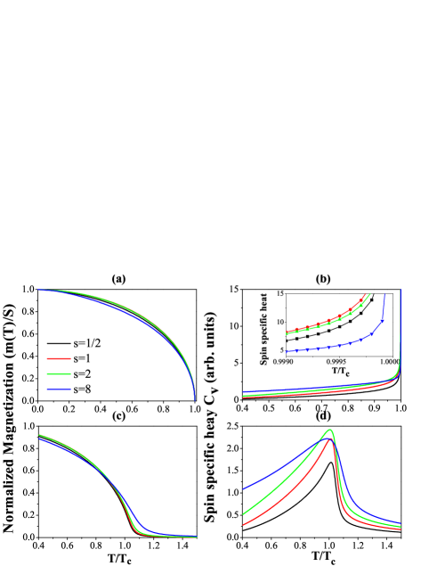
Figure 1: (Color online) Temperature dependence of (a) magnetization and (b) specific heat (arbitrary unit) for spin=1/2,1,2,8 in the absence of the external field; Temperature dependence of (c) magnetization and (d) specific heat for spin=1/2,1,2,8 in an external field $H/T_{c}=0.001$.

IV Dynamic Equations

The energy or heat transfer among electrons, spins and lattice may be captured by the general rate equations given below,

$$\frac{d\mathcal{E}_{e}}{dt} = -\Gamma_{es}-\Gamma_{el}$$ (16)

$$\frac{d\mathcal{E}_{l}}{dt} = \Gamma_{sl}+\Gamma_{el}$$ (17)

$$\frac{d\mathcal{E}_{s}}{dt} = \Gamma_{es}-\Gamma_{sl}$$ (18)

where ${\cal E}_{i}$ are the energy densities ($i=e,s,l$) and the rate of the energy transfer $\Gamma_{ij}$ should be determined by Eq. (1). Since we have neglected the weaker interaction between spins and lattice, we set $\Gamma_{sl}=0$ in the above equations. In the following, we explicitly derive the relaxation rates of $\Gamma_{el}$ and $\Gamma_{es}$ from Eqs. (3) and (5).

IV.1 Electron-lattice relaxation $\Gamma_{el}$

The energy transfer rate between electrons and phonons does not involve the spin. The Fermi golden rule applied to Eq. (3) immediately leads to

$$\Gamma_{el} = \frac{4\pi}{\hbar}\sum_{{\bf k},{\bf q}}\hbar\omega_{\bf q}^{p}|B_{\bf q}|^{2}\delta(\epsilon_{\bf k}-\epsilon_{\bf k+q}+\hbar\omega_{\bf q}^{p})\times$$

$$(n_{\bf k+q}(1-n_{\bf k})(1+n_{\bf q}^{p})-n_{\bf k}(1-n_{\bf k+q})n_{\bf q}^{p}),$$

where the first (second) term represents the energy transfer from (to) the electrons to (from) lattice by emitting (absorbing) a phonon. Note that the electrons and phonons have different temperatures; otherwise the detailed balance will make the net energy transfer zero. The electron and phonon densities are given by their respective equilibrium temperatures at $T_{s}$ and $T_{l}$, i.e., $n_{\bf k}=[\exp((\epsilon_{\bf k}-\epsilon_{F})/k_{B}T_{e})+1]^{-1}$ and $n_{\bf q}^{p}=[\exp(\hbar\omega_{\bf q}^{p}/k_{B}T_{l})-1]^{-1}$. We consider polarization-independent acoustic phonons, i.e., $\omega_{\bf q}^{p}=v_{s}q$ where $v_{s}$ is the phonon velocity. By replacing $B_{\bf p}$ given in Eq. (4) into Eq. (19), we have

$$\Gamma_{el}=\frac{4\pi}{\hbar}\left(\frac{2}{3}\epsilon_{F}\right)^{2}\frac{V}{(2\pi)^{4}}\frac{m_{e}}{\hbar}\frac{m_{e}}{M}\int_{0}^{q_{m}}q^{3}dq\frac{e^{\frac{\hbar v_{s}q}{k_{B}T_{l}}}-e^{\frac{\hbar v_{s}q}{k_{B}T_{e}}}}{e^{\frac{\hbar v_{s}q}{k_{B}T_{l}}}-1}\int_{\epsilon_{\bf q}}^{+\infty}\frac{e^{\frac{\epsilon-\epsilon_{F}}{k_{B}T_{e}}}d\epsilon}{(e^{\frac{\hbar v_{s}q}{k_{B}T_{e}}}e^{\frac{\epsilon-\epsilon_{F}}{k_{B}T_{e}}}+1)(e^{\frac{\epsilon-\epsilon_{F}}{k_{B}T_{e}}}+1)},$$ (20)

where we have defined the cut-off energy $\epsilon_{\bf q}\equiv(q-\frac{2m}{\hbar^{2}}\hbar v_{s})^{2}\frac{\hbar^{2}}{2m}$ which comes from the $\delta$ function, and we have introduced the maximum phonon wave number in the First Brillouin zone (this definition is the same for magnons and Fermi wave vectors), $q_{m}=k_{F}=(6\pi^{2})^{1/3}/a_{0}$. By integrating over the electron energy $\epsilon$, we obtain

$$\Gamma_{el}=\frac{4\pi}{\hbar}\left(\frac{2}{3}\epsilon_{F}\right)^{2}\frac{V}{(2\pi)^{4}}\frac{m_{e}}{\hbar}\frac{m_{e}}{M}\int_{0}^{q_{m}}q^{3}dq(n_{\bf q}^{p}(T_{e})-n_{\bf q}^{p}(T_{l}))k_{B}T_{e}\left(\frac{\hbar v_{s}q}{k_{B}T_{e}}-\ln\left(\frac{e^{\frac{\hbar v_{s}q}{k_{B}T_{e}}}e^{\frac{\epsilon_{\bf q}-\epsilon_{F}}{k_{B}T_{e}}}+1}{e^{\frac{\epsilon_{\bf q}-\epsilon_{F}}{k_{B}T_{e}}}+1}\right)\right),$$ (21)

where we have defined a Debye temperature, $\theta=\hbar v_{s}q_{m}/k_{B}$. The last term of Eq. (21) can be approximated by

$$\left(\frac{\hbar v_{s}q}{k_{B}T_{e}}-\ln\left(\frac{e^{\frac{\hbar v_{s}q}{k_{B}T_{e}}}e^{\frac{\epsilon_{\bf q}-\epsilon_{F}}{k_{B}T_{e}}}+1}{e^{\frac{\epsilon_{\bf q}-\epsilon_{F}}{k_{B}T_{e}}}+1}\right)\right)\approx\frac{\hbar v_{s}q}{k_{B}T_{e}}\Theta(2k_{F}-p),$$ (22)

for $\hbar\omega_{\bf q}\ll k_{B}T_{e}$, where $\Theta(x)$ is the step function. Therefore, the relaxation rate becomes

$$\Gamma_{el}=\frac{1}{\hbar}\left(\frac{2}{3}\epsilon_{F}\right)^{2}\frac{9\pi}{2V}\frac{m_{e}}{M}\frac{\theta}{T_{F}}\left[G_{4}\left(\frac{T_{e}}{\theta}\right)-G_{4}\left(\frac{T_{l}}{\theta}\right)\right]$$ (23)

and $G_{n}(x)=x^{n+1}\int_{0}^{1/x}t^{n}dt/(e^{t}-1)$.

Interestingly, for $T_{e},T_{l}\gtrsim\theta$, the relaxation rate reduces to:

$$\Gamma_{el}=\frac{1}{\hbar}\left(\frac{2}{3}\epsilon_{F}\right)^{2}\frac{9\pi}{8V}\frac{m_{e}}{M}\left(\frac{T_{e}-T_{l}}{T_{F}}\right).$$ (24)

Thus, the relaxation rate is simply proportional to the difference between the electron and lattice temperatures($\Gamma_{el}\propto T_{e}-T_{l}$); this is the assumption made in the earlier three temperature model beaurepaire .

IV.2 Electron-spin relaxation $\Gamma_{es}$

The interaction between the electrons and spins given by Eq. (5) may be simplified by using the self-consistent random phase approximation, i.e., we replace ${\hat{S}}_{i}^{z}$ by its thermal average $m(T_{s})$ and ${\hat{S}}_{\bf q}^{\pm}=\sqrt{2m(T_{s})}a_{\bf q}^{\mp}$. The electron-spin interaction can then be rewritten as

$${\hat{H}}_{es} = -\frac{J_{ex}}{\sqrt{N}}\sqrt{2Sm(T_{s})}\sum_{{\bf k}{\bf q}}({\hat{c}}^{+}_{{\bf k}-{\bf q}\uparrow}{\hat{c}}_{{\bf k}\downarrow}{\hat{a}}_{\bf q}+{\hat{c}}^{+}_{{\bf k}+{\bf q}\downarrow}{\hat{c}}_{{\bf k}\uparrow}{\hat{a}}_{\bf q}^{+}),$$

where we have dropped the $m(T)\sigma_{z}$ term since it does not involve the energy transfer between the electron and the spin.

The second order perturbation immediately leads to the electron-spin relaxation:

$$\Gamma_{es} = \frac{2\pi}{\hbar}\frac{2Sm(T_{s})}{N}J_{ex}^{2}\sum_{{\bf k},{\bf q}}\hbar\omega_{\bf q}\delta(\epsilon_{\bf k}-\epsilon_{{\bf k}-{\bf q}}-\hbar\omega_{\bf q})$$

$$\times (n_{{\bf k}\downarrow}(1-n_{{\bf k}-{\bf q}\uparrow})(1+n_{\bf q}^{s})-n_{{\bf k}-{\bf q}\uparrow}(1-n_{{\bf k}\downarrow})n_{\bf q}^{s})$$

where $\omega_{\bf q}$ is the magnon frequency given by Eq. (10), the electron distribution is $n_{\bf k\sigma}=[\exp((\epsilon_{\bf k}-\epsilon_{F})/k_{B}T_{e})+1]^{-1}$ and the magnon distribution is $n_{\bf q}^{s}=[\exp(\hbar\omega_{\bf q})-1]^{-1}$. Note that the electron sub-system is considered unpolarized due to the strong spin relaxation occuring during thermalization. In Eq. (26), the first (second) term represents the electron emitting (absorbing) a magnon. For the long wavelength, the magnon dispersion, Eq. (10), is simply $\hbar\omega_{\bf q}=\mu_{B}H_{ext}+\alpha k_{B}T_{c}q^{2}a_{0}^{2}$ where $\alpha\approx 1$. Following the same procedure as the previous section, we find,

$$\Gamma_{es}=\frac{4\pi}{\hbar}2SM(T_{s})J_{ex}^{2}\frac{V}{(2\pi)^{4}}\frac{m^{2}}{\hbar^{4}}$$

$$\times\int_{0}^{q_{m}}qdq(\hbar\omega_{\bf q})^{2}(n_{\bf q}^{s}(T_{e})-n_{\bf q}^{s}(T_{s}))$$ (27)

If the magnetic field is zero, the integration over $q$ can be immediately carried out and we approximately have (discard the numerical constant $\alpha$)

$$\Gamma_{es}=\frac{(6\pi^{2})^{10/3}J_{ex}^{2}m^{3}(T_{s})}{2\hbar V}\left(\frac{T_{c}}{T_{F}}\right)^{2}$$

$$\times\left[G_{2}\left(\frac{T_{e}}{DT_{c}}\right)-G_{2}\left(\frac{T_{s}}{DT_{c}}\right)\right]$$ (28)

where $G_{n}(x)$ has been defined below Eq. (23) and the temperature-dependent spin stiffness is $D=m(T_{s})q_{m}^{2}a^{2}$. An important result of this paper is that $\Gamma_{es}$ is proportional to $m^{3}(T_{s})$ and thus it is vanishingly small near the Curie temperature. Furthermore, since $T_{e}/T_{c}$ and $T_{s}/T_{c}$ are always comparable to 1, the electron-spin relaxation rate given by Eq. (28) is not proportional to $T_{e}-T_{s}$, which is quite different from the previous three-temperature model beaurepaire .

IV.3 Specific heats of subsystems

As the right sides of the rate equations, Eqs. (16)-(18), are expressed in terms of three temperatures $T_{e}$, $T_{s}$ and $T_{l}$, we need to relate the energy change of each system to the temperatures, i.e., we should define the heat capacities $C_{i}$ for each subsystem $d{\mathcal{E}_{i}}=C_{i}dT_{i}$. The specific heat depends on the material details. To be more specific, we consider the Ni metal that has been experimentally investigated most extensively.

Specific heat of the electrons

In a free electron picture, the specific heat of an electron gas is $C_{e}=\frac{1}{2}\pi n_{e}k_{B}(T_{e}/T_{F})(1-3\pi^{2}/10(T_{e}/T_{F})^{2}-...)$, where $n_{e}$ is the electron density and $T_{F}$ is the Fermi temperature kittel . However, this approximation is usually poor in the case of transition metals. In our model, we assume that the electron specific heat remains proportional to the temperature $C_{e}=\gamma_{e}T_{e}$ where $\gamma_{e}\approx 1.5\times 10^{3}$Jm^-3K^-2 is taken from experiments heat , which is smaller than the one assumed earlier beaurepaire .

Specific heat of lattice

The phonon energy is derived from the Debye model, $E_{p}=\int d^{3}{\bf q}\hbar\omega_{\bf q}^{p}n_{\bf q}^{p}(T)$. This yields $C_{l}=3N_{A}k_{B}F_{D}(T_{D}/T)$, where $N_{A}$ is the Avogadro number and $F_{D}=\int_{0}^{T_{D}/T}x^{4}e^{x}/(e^{x}-1)^{2}dx$ is the Debye function. This form of the lattice specific heat is consistent with Pawel et al. heat .

Specific heat of the spins

We determine the spin specific heat from the numerical derivative of the spin energy Eq. (15), as explicitly calculated in Sec.  III. In Fig. 1(b) and Fig. 1(d), we have already shown the temperature dependence of the spin specific heat with and without the external field.

IV.4 Summary

We summarize below the dynamic equations that govern the time-dependence of the three subsystem temperatures after the laser pumping,

$$C_{e}(T_{e})\frac{dT_{e}}{dt} = -\Gamma_{el}(T_{e},T_{l})-\Gamma_{es}(T_{e},T_{s})+P(t)$$ (29)

$$C_{l}(T_{l})\frac{dT_{l}}{dt} = \Gamma_{el}(T_{e},T_{l})-\frac{T_{l}-T_{rm}}{\tau_{l}}$$ (30)

$$C_{s}(T_{s})\frac{dT_{s}}{dt} = \Gamma_{es}(T_{e},T_{s})$$ (31)

where we have used $d\mathcal{E}_{\mu}/dt=C_{\mu}(T_{\mu})dT_{\mu}/dt$ and we have discarded the spin-phonon interaction. In Eq. (29) we have inserted $P(t)$ representing the initial laser energy transfer to the electrons and in Eq. (30), we have included a phenomenological heat diffusion of phonons to environment which is set at the room temperature $T_{rm}$, this term becomes significant only at long time scale (subnanoseconds). The functions $\Gamma_{ij}$ are:

$$\Gamma_{el} = W_{el}\left[G_{4}\left(\frac{T_{e}}{\theta_{D}}\right)-G_{4}\left(\frac{T_{l}}{\theta_{D}}\right)\right]$$ (32)

$$\Gamma_{es} = W_{es}m^{3}(T_{s})\left[G_{2}\left(\frac{T_{e}}{DT_{c}}\right)-G_{2}\left(\frac{T_{s}}{DT_{c}}\right)\right]$$ (33)

where the constants $W_{el}$ and $W_{es}$ are given in Eq. (24) and (28), and $D=(6\pi^{2})^{1/3}m(T_{s})$

V Numerical results

In this Section, we numerically solve our central Eqs. (29)-(34) for a number of plausible material parameters. Our particular focus will be on the difference between our model and the previous three-temperature model. Since the demagnetization is mainly controlled by the interaction between electrons and spins, we choose a set of different $J_{ex}$–a large $J_{ex}$ representing transition metals (e.g., Ni, Fe and Co) and a weak $J_{ex}$ for some ferromagnetic oxides and dilute magnetic semiconductors. Equations (29)-(31) are solved by using the following procedure. First, we assume that the laser instantaneously heats the electron bath to $T_{e}(0)$ while the spin and lattice temperatures remain at the room temperature $T_{s}(0)=T_{l}(0)=T_{rm}$. With these initial conditions, we compute these temperatures after $t>0$ where the laser source has been turned off $P(t>0)=0$. If we only consider the time scale smaller than 100ps we may drop the heat diffusion term in Eq. (30).

In Fig. 2, we show the typical temperature profiles after a low intensity laser pumping. In general, the electron-spin interaction is stronger than the electron-phonon interaction at low temperature, and spin and electron temperatures equilibrate within subpicoseconds. It takes an order of magnitude longer to reach the equilibrium between lattice and the electrons. Also shown in the inset is the time dependent magnetization which illustrates the fast demagnetization and slow remagnetization. In Fig. 3, we show the temperature dependence of magnetization for different $J_{ex}$. As expected, the demagnetization time scales with the inverse of $J_{ex}$ while the remagnetization is independent of $J_{ex}$ since the latter is controlled by the electron-lattice interaction.

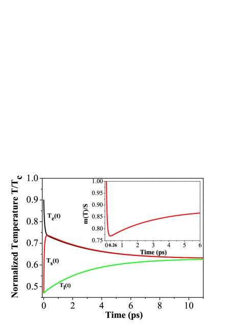
Figure 2: (Color online) Time dependence of the temperatures of the electrons, spins and lattice after irradiation by a low intensity laser with $T_{e}(0)=0.7T_{c}$, and $T_{s}(0)=T_{p}(0)=T_{rm}=0.47T_{c}$, and $T_{c}=620$K. The inset shows the minimum magnetization (or maximum spin temperature) occurs at about 260 femtosecond. The other parameters are: $J_{ex}=0.15$eV, $\epsilon_{F}=8$eV, , $M/m=10^{5}$, and $a_{0}=0.25$nm.

Figure 3: (Color online) Time-dependent magnetization as a function of time in logarithmical scale for various exchange parameters at a fixed laser-fluence. The parameters are same as those of Fig. 2.

A much more interesting case is the high intensity of laser pumping. In this case, the spin temperature raises to the Curie temperature in 0.1-0.2 ps as shown in Fig. 4. Due to vanishingly small magnetization at the Curie temperature, the energy transfer between electrons and spins becomes negligible and thus the spin temperature stays constant for an extended period of time (a few ps). The electron temperature, however, continues to decrease due to the electron-lattice interaction which is not affected by the dynamic slowdown of the spins. Interestingly, after the electron temperature drops below the spin temperature, the spin system begins to heat the electron system and thus the electron temperature behaves non-monotonically as seen in Fig. 4.

The dynamic slowdown of the spin temperature shown in Fig. 4 is a general property of critical phenomena. Due to the disappearance of the order parameter (the magnetization $m(T)$ in present case), the effective interaction reduces to zero at the critical point. In Fig. 5, we show the time interval (labeled in Fig. 5) for the critical slowdown as a function of the maximum spin temperature $T_{m}$ for a given laser pumping power. As it is expected, the critical slowdown shows a power law, $\tau_{s}\propto[1-T_{m}/T_{c}]^{-\delta}$ with the exponent $\delta$ depending on $J_{ex}$. In the case of very high intensity of the laser pumping, $T_{m}$ can be very close to $T_{c}$ and the magnetization dynamics can be extremely slow. In the presence of the external field, however, the spin system does not have a sharp phase transition anymore and the critical slowdown is removed, i.e., one recovers the fast magnetization dynamics. In Fig. 6, we compare the magnetization dynamics with and without the magnetic field. The magnetic field suppresses the dynamic slowdown.

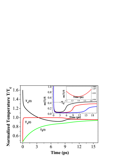
Figure 4: (Color Online) Time evolution of three temperature for a large laser-fluence case $T_{e}(0)=1.6$. The critical slowing down of the spin system is identified as the plateau in the figure. The inset defines a slowdown time $\tau_{d}$. The smaller inset shows the magnified region in the vicinity of the maximum temperature. The other parameters are same as those in Fig. 2.

Figure 5: (Color online) Log-log plot of $\tau_{d}$ versus the reduced temperature for $J_{ex}=0.1$ and 0.2. The exponents are $\delta=0.43$ and $\delta=0.34$ respectively. The parameters are same as those in Fig. 4. The dashed line is for eye-guidance.

Figure 6: (Color online) Magnetization as a function of time with and without the magnetic field. The parameters are same as those in Fig. 4.

Finally, Fig. 7 shows the exponential dependence of $\tau_{d}$ on the initial electron temperature which is directly related to the pumping laser fluence.

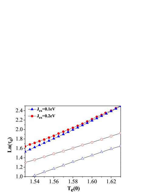
Figure 7: (Color online) Log($\tau_{d}$) versus the initial electron temperature for two values of $J_{ex}$ with (open symbols) and without (filled symbols) the magnetic field. $T_{e}(0)$ is normalized initial electron temperature.

VI Discussion

VI.1 Connection with experiments on LID

We now comment on the connection of our theory to the existing experimental results. The LID experiments performed on transition metallic ferromagnets beaurepaire ; koop ; carpene are usually at low laser pumping power. In these experiments, the previous phenomenological three temperature model provides an essential interpretation of demagnetization: the laser induced hot electrons transfer their energies to spins and lattice. As discussed in Sec. II, in our model, the demagnetization (i.e., loss of spin memory) occurs during the instantaneous thermalization of the interacting baths. Therefore, the demagnetization/remagnetization time scale is governed by energy transfer between the baths: the demagnetization is given by the electron-spin interaction while remagnetization time is determined by the electron-phonon interactions.

For transition metals, the electron-spin interaction is at least several times larger than the electron-phonon interaction. Thus, the demagnetization is faster than the remagnetization. For half-metals and oxidized ferromagnets, the demagnetization is usually longer due to a reduced electron-spin interaction. When the temperature increases, the demagnetization time could be significantly increased kise ; this is due to the weakening of the effective electron-spin interaction with a reduced magnetization. As the temperature approaches the Curie temperature, Ogasawara et al. osagawara observed that in all their samples, the demagnetization time could be enhanced by one order of magnitude.

The influence of the pump intensity on the demagnetization time can be similarly understood. As we have shown, a large pumping intensity creates high temperature electrons which heat the spin temperature to the Curie temperature. Thus the temperature and the pumping intensity dependence of the demagnetization involve the exact physics of critical slowdown.

VI.2 Connection with HAMR

HAMR involves heating ferromagnets to an elevated temperature so that a moderate magnetic field is able to overcome the magnetic anisotropy for magnetization reversal. Since the time scale in HAMR processes is of the order of nanoseconds, the dynamics studied here can be viewed as ultrafast, i.e., all three temperatures have already reached equilibrium for HAMR dynamics. Even for the temperature close to the Curie temperature, the dynamics slowdown remains “ultrafast” for HAMR as long as a moderate magnetic field is present. Thus, the HAMR dynamics could be performed in two distinct time scales: a fast dynamics within 10 picoseconds which determines the longitudinal magnetization $m(T)$ and a slow dynamics from subnanoseconds to a few nanoseconds which determines the direction of the magnetization by the conventional Landau-Lifshitz-Gilbert equation. The detail calculations for HAMR dynamics will be published elsewhere.

VII Conclusion

We have proposed a microscopic approach to the three temperature model applied to laser-induced ultrafast demagnetization. The microscopic model consists of interactions among laser-excited electrons, collective spin excitations and lattice. Under the assumption of instantaneous spin memory loss during the baths thermalization, the demagnetization problem reduces to energy transfer between the thermalized baths.

A self-consistent random phase approximation is developed to model the low excitation of the spin system for a wide range of temperatures. A set of dynamic equations for the time-dependent temperatures of electrons, spins and lattice are explicitly expressed in terms of the microscopic parameters. While the resulting equations are similar to the phenomenological three-temperature model, there are important distinctions in the temperature dependent properties. In particular, the magnon softening plays a key role in demagnetization near Curie temperature where a significant slowdown of the spin dynamics occurs. We have also shown that for sufficiently high temperatures (above the Debye temperature), the dynamic properties are governed by only a few parameters: the Curie and Fermi temperatures, the electron-spin exchange integral $J_{ex}$, and the electron-phonon coupling constant $B_{\bf q}$. The magnetization dynamic near the Curie temperature is rather universal. Our numerical study of these equations illustrates that, due to the reduction of the average magnetization as a function of the spin temperature, both pump intensity and sample temperature are responsible for a relative long demagnetization (several picoseconds). An external magnetic field can suppress the critical dynamic slowdown.

- (1) E. Beaurepaire, J.-C. Merle, A. Daunois and J.-Y. Bigot, Phys. Rev. Lett. 76, 4250 (1996).
- (2) C. D. Stanciu, F. Hansteen, A.V. Kimel, A. Kirilyuk, A. Tsukamoto, A. Itoh, and Th. Rasing, Phys. Rev. Lett. 99, 047601 (2007).
- (3) W. A. Challener, C. Peng, A. V. Itagi, D. Karns, W. Peng, Y. Peng, X.M. Yang, X. Zhu, N. J. Gokemeijer, Y.-T. Hsia, G. Ju, R. E. Rottmayer, M. A. Seigler and E. C. Gage, Nature Photonics 3, 220-224 (2009).
- (4) B. Koopmans, J.J.M. Ruigrok, F. Dalla Longa, and W.J.M. de Jonge, Phys. Rev. Lett. 95, 267207 (2005); B. Koopmans, H.H.J.E. Kicken, M. van Kampen, and W.J.M. de Jonge, J. Magn. Magn. Mater. 286, 271-275 (2005).
- (5) B. Koopmans, G. Malinowski, F. Dalla Longa, D. Steiauf, M. F hnle, T. Roth, M. Cinchetti and M. Aeschlimann, Nature Materials (2009).
- (6) E. Carpene, E. Mancini, C. Dallera, M. Brenna, E. Puppin, and S. De Silvestri, Phys. Rev. B 78, 174422 (2008).
- (7) T. Ogasawara, K. Ohgushi, Y. Tomioka, K. S. Takahashi, H. Okamoto, M. Kawasaki, and Y. Tokura, Phys. Rev. Lett. 94, 087202 (2005).
- (8) T. Kise, T. Ogasawara, M. Ashida, Y. Tomioka, Y. Tokura, and M. Kuwata-Gonokami, Phys. Rev Lett. 85, 1986 (2000).
- (9) G. M. Muller, J. Walowski, M. Djordjevic, G.-X. Miao, A. Gupta, A. V. Ramos, K. Gehrke, V. Moshnyaga, K. Samwer, J. Schmalhorst, A. Thomas, A. Hutten, G. Reiss, J. S. Moodera and M. Münzenberg, Nature Material 8, 56 (2009).
- (10) Q. Zhang, A.V. Nurmikko, G.X. Miao, G. Xiao and A. Gupta, Phys. Rev. B 74, 064414 (2006).
- (11) J. Wang, C. Sun, J. Kono, A. Oiwa, H. Munekata, L. Cywinski, and L. J. Sham, Phys. Rev. Lett. 95, 167401 (2005); J. Wang, I. Cotoros, K. M. Dani, X. Liu, J. K. Furdyna, and D. S. Chemla, Phys. Rev. Lett. 98, 217401 (2007).
- (12) A. Kirilyuk, A. V. Kimel, and T. Rasing, Rev. Mod. Phys. 82, 2731 (2010).
- (13) G. P. Zhang and W. Hu bner, Phys. Rev. Lett. 85, 3025 (2000).
- (14) D. Steiauf and M. Fahnle, Phys. Rev. B 79, 140401(R) (2009).
- (15) W. Hübner and K. H. Bennemann, Phys. Rev. B 53, 3422 (1996).
- (16) L. Cywinski and L. J. Sham, Phys. Rev. B 76, 045205 (2007); J. Wang, L. Cywinski, C. Sun, J. Kono, H. Munekata, and L.J. Sham Phys. Rev. B 77, 235308 (2008).
- (17) T. Hartenstein, G. Lefkidis, W. Hübner, G. P. Zhang, and Y. Bai, J. Appl. Phys. 105, 07D305 (2009).
- (18) B. Koopmans, M. van Kampen, J. T. Kohlhepp, and W. J. M. de Jonge, Phys. Rev. Lett. 85, 844 (2000).
- (19) M. Battiato, K. Carva, and P. M. Oppeneer, Phys. Rev. Lett. 105 027203 (2010).
- (20) U. Atxitia, O. Chubykalo-Fesenko, J. Walowski, A. Mann, and M. Münzenberg, Phys. Rev. B 81, 174401 (2010).
- (21) R. J. Elliott, Phys. Rev. 96, 266 (1954).
- (22) Y. Yafet, in Solid State Physics, edited by F. Seitz and D. Turnbull (Academic Press, New York, 1963), Vol. 14; A.W. Overhauser, Phys. Rev. 89 689 (1953).
- (23) P.M. Echenique, J.M. Pitarke,E.V. Chulkov, and A. Rubio, Chem. Phys. 251, 1 (2000); R. Knorren, G. Bouzerar, and K.H. Bennemann, J. Phys.: Cond. Matter 14, R739 (2002).
- (24) M.I. D’yakonov, V.I. Perel’, Zh. Eksp. Teor. Fiz. 60, 1954 (1971); Fiz. Tverd. Tela (Leningrad) 13, 3581 (1971).
- (25) G.L. Bir, A.G. Aronov, G.E. Pikus, Zh. Eksp. Teor. Fiz. 69, 1382 (1975).
- (26) C. W. Hass, and H. B. Callen, ”Ferromagnetic relaxation, and resonance line widths”, in Magnetism, edited by G.T. Rado, Academic press (New York and London), (1963).
- (27) C. Boeglin, E. Beaurepaire, V. Halte, V. Lopez-Flores, C. Stamm, N. Pontius, H. A. Durr and J.-Y. Bigot, Nature 465, 458 (2010).
- (28) J.-Y. Bigot, M. Vomir and E. Beaurepaire, Nature Physics 5, 515 (2009).
- (29) D. Pines, Elementary excitations in solids, Westview Press, 1999. See also J.M. Ziman, Electrons and phonons, Oxford, Classic Texts, 2001.
- (30) J.H. Van Vleck, Phys. Rev. 57, 426 (1940); R. D. Mattuck and M.W.P. Strandberg, Phys. Rev. 119, 1204 (1960).
- (31) A. B. Schmidt, M. Pickel, M. Donath, P. Buczek, A. Ernst, V.P. Zhukov, P. M. Echenique, L. M. Sandratskii, E. V. Chulkov, and M. Weinelt, Phys. Rev. Lett. 105 197401 (2010).
- (32) N. W. Ashcroft and N. D. Mermin, Solid State Physics, (Holt, Rinehart and Winston, New York), 1976.
- (33) S. V. Tyablikov, Methods in the quantum theory of magnetism (Plenum Press, 1967).
- (34) G. V. Vasyutinskii and A. A. Kazakov, Theor. Math. Phys. 95, 450 (1993).
- (35) C. Kittel, Introduction to Solid State Physics, 4th Ed. (John Wiley & Sons, New York) (1971).
- (36) D. L.Connelly, J. S. Loomis, and D. E. Mapother, Phys. Rev. B 3, 924 (1971); R.E. Pawel and E.E. Stansbury, J. Phys. Chem. Solids 26, 757 (1965).