The Berry Phase for Simple Harmonic Oscillators

Abstract.

We evaluate the Berry phase for a “missing” family of the square integrable wavefunctions for the linear harmonic oscillator, which cannot be derived by the separation of variables (in a natural way). Instead, it is obtained by the action of the maximal kinematical invariance group on the standard solutions. A simple closed formula for the phase (in terms of elementary functions) is found by integration with the help of a computer algebra system.

Recent reports on observations of the dynamical Casimir effect [27], [51] strengthens the interest to ‘nonclassical’ states in quantum optics and generalized harmonic oscillators [10], [11], [13], [14], [15], [17], [33], [34] and [37]. The amplification of quantum fluctuations by modulating parameters of an oscillator is closely related to the process of particle production in quantum fields [11], [24], [34] and [37]. Other dynamical amplification mechanisms include the Unruh effect [47] and Hawking radiation [20], [21].

The purpose of this paper is to evaluate the Berry phase for certain “missing” solutions of the time-dependent Schrödinger equation for the linear harmonic oscillator as an instructive example. Applications will be discussed elsewhere.

1. Hidden Solutions

The time-dependent Schrödinger equation for the simple harmonic oscillator,

$$2i\psi_{t}+\psi_{xx}-x^{2}\psi=0,$$ (1.1)

has the following six-parameter family of (square integrable) solutions [32]:

$$\psi_{n}\left(x,t\right)=\frac{e^{i\left(\alpha\left(t\right)x^{2}+\delta\left(t\right)x+\kappa\left(t\right)\right)+i\left(2n+1\right)\gamma\left(t\right)}}{\sqrt{2^{n}n!\mu\left(t\right)\sqrt{\pi}}}\ e^{-\left(\beta\left(t\right)x+\varepsilon\left(t\right)\right)^{2}/2}\ H_{n}\left(\beta\left(t\right)x+\varepsilon\left(t\right)\right),$$ (1.2)

where $H_{n}\left(x\right)$ are the Hermite polynomials [40] and

$$\mu\left(t\right) = \mu_{0}\sqrt{\beta_{0}^{4}\sin^{2}t+\left(2\alpha_{0}\sin t+\cos t\right)^{2}},$$ (1.3)

$$\alpha\left(t\right) = \frac{\alpha_{0}\cos 2t+\sin 2t\ \left(\beta_{0}^{4}+4\alpha_{0}^{2}-1\right)/4}{\beta_{0}^{4}\sin^{2}t+\left(2\alpha_{0}\sin t+\cos t\right)^{2}},$$ (1.4)

$$\beta\left(t\right) = \frac{\beta_{0}}{\sqrt{\beta_{0}^{4}\sin^{2}t+\left(2\alpha_{0}\sin t+\cos t\right)^{2}}},$$ (1.5)

$$\gamma\left(t\right) = \gamma_{0}-\frac{1}{2}\arctan\frac{\beta_{0}^{2}\sin t}{2\alpha_{0}\sin t+\cos t},$$ (1.6)

$$\delta\left(t\right) = \frac{\delta_{0}\left(2\alpha_{0}\sin t+\cos t\right)+\varepsilon_{0}\beta_{0}^{3}\sin t}{\beta_{0}^{4}\sin^{2}t+\left(2\alpha_{0}\sin t+\cos t\right)^{2}},$$ (1.7)

$$\varepsilon\left(t\right) = \frac{\varepsilon_{0}\left(2\alpha_{0}\sin t+\cos t\right)-\beta_{0}\delta_{0}\sin t}{\sqrt{\beta_{0}^{4}\sin^{2}t+\left(2\alpha_{0}\sin t+\cos t\right)^{2}}},$$ (1.8)

$$\kappa\left(t\right) = \kappa_{0}+\sin^{2}t\ \frac{\varepsilon_{0}\beta_{0}^{2}\left(\alpha_{0}\varepsilon_{0}-\beta_{0}\delta_{0}\right)-\alpha_{0}\delta_{0}^{2}}{\beta_{0}^{4}\sin^{2}t+\left(2\alpha_{0}\sin t+\cos t\right)^{2}}$$

$$+\frac{1}{4}\sin 2t\ \frac{\varepsilon_{0}^{2}\beta_{0}^{2}-\delta_{0}^{2}}{\beta_{0}^{4}\sin^{2}t+\left(2\alpha_{0}\sin t+\cos t\right)^{2}}$$

($\mu_{0}\neq 0,$ $\alpha_{0},$ $\beta_{0}\neq 0,$ $\gamma_{0},$ $\delta_{0},$ $\varepsilon_{0},$ $\kappa_{0}$ are real initial data). These solutions have been derived analytically in the framework of a unified approach to generalized harmonic oscillators (see, for example, [8], [9], [29], [52], [53] and the references therein). They are also verified by a direct substitution with the aid of Mathematica computer algebra system [26], [31]. (The simplest special case $\mu_{0}=\beta_{0}=1$ and $\alpha_{0}=\gamma_{0}=\delta_{0}=\varepsilon_{0}=\kappa_{0}=0$ reproduces the textbook solution obtained by the separation of variables [42], [18], [28], [35]. The shape-preserving oscillator evolutions occur when $\alpha_{0}=0$ and $\beta_{0}=1$ and a special case when $\alpha_{0}=0$ is discussed in [22]. More details on the derivation of these formulas and some Mathematica animations, revealing a new feature – an oscillation in space of the probability density $\left|\psi\left(x,t\right)\right|^{2}$ – of these solutions, can be found in Refs. [26], [30] and [31].)

The “dynamic harmonic oscillator states” (1.2)–(1) are eigenfunctions,

$$E\left(t\right)\psi_{n}\left(x,t\right)=\left(n+\frac{1}{2}\right)\psi_{n}\left(x,t\right),$$ (1.10)

of the time-dependent quadratic invariant,

$$E\left(t\right)=\frac{1}{2}\left[\frac{\left(p-2\alpha x-\delta\right)^{2}}{\beta^{2}}+\left(\beta x+\varepsilon\right)^{2}\right],\qquad\frac{d}{dt}\langle E\rangle=0,$$ (1.11)

where $p=i^{-1}\partial/\partial x$ and the required operator identity,

$$\frac{\partial E}{\partial t}+i^{-1}\left[E,H\right]=0,\qquad H=\frac{1}{2}\left(p^{2}+x^{2}\right),$$ (1.12)

holds [41].

The (isomorphic) maximum kinematical invariance groups of the free particle and harmonic oscillator were introduced in [1], [2], [19], [23], [38] and [39] (see also [7], [25], [36], [48] and the references therein). We have established a connection with certain Ermakov-type system which allows us to bypass a complexity of the traditional Lie algebra approach [30], [32]. (A general procedure of obtaining new solutions by acting on any set of given ones by enveloping algebra of generators of the Heisenberg–Weyl group is described in [15]; see also [3], [4] and [14].)

2. Evaluation of the Phase

The holonomic effect in quantum mechanics known as Berry’s phase [5], [6], [43], [50] has received considerable attention over the years (see, for example, [16], [49] and the other references in [41]). The derivative of Berry’s phase has been recently calculated for the generalized harmonic oscillators as follows [41]:

$$\frac{d\theta_{n}}{dt}=-\beta^{-2}\left(\varepsilon^{2}+n+\frac{1}{2}\right)\frac{d\alpha}{dt}+\varepsilon\beta^{-1}\frac{d\delta}{dt}-\frac{d\kappa}{dt},$$ (2.1)

where we are going to use (1.4)–(1) and simplify. Integrating by parts, one gets

$$\theta_{n} = -\left(n+\frac{1}{2}\right)\int\beta^{-2}\frac{d\alpha}{dt}\ dt-\left(\frac{\varepsilon}{\beta}\right)^{2}\alpha+\frac{\varepsilon\delta}{\beta}-\kappa$$

$$+\int\left[\alpha\frac{d}{dt}\left(\frac{\varepsilon}{\beta}\right)^{2}-\delta\frac{d}{dt}\left(\frac{\varepsilon}{\beta}\right)\right]\ dt.$$

Here,

$$4\beta_{0}^{2}\left[\left(\frac{\varepsilon}{\beta}\right)^{2}\alpha-\frac{\varepsilon\delta}{\beta}+\kappa\right]=2\beta_{0}\left(2\beta_{0}\kappa_{0}-\delta_{0}\varepsilon_{0}\right)$$ (2.3)

$$\qquad+2\varepsilon_{0}\left(2\alpha_{0}\varepsilon_{0}-\beta_{0}\delta_{0}\right)\cos 2t+\left[\left(2\alpha_{0}\varepsilon_{0}-\beta_{0}\delta_{0}\right)^{2}-\varepsilon_{0}^{2}\right]\sin 2t,$$

$$4\beta_{0}^{2}\int\left[\alpha\frac{d}{dt}\left(\frac{\varepsilon}{\beta}\right)^{2}-\delta\frac{d}{dt}\left(\frac{\varepsilon}{\beta}\right)\right]\ dt=2t\left[\left(2\alpha_{0}\varepsilon_{0}-\beta_{0}\delta_{0}\right)^{2}+\varepsilon_{0}^{2}\right]$$ (2.4)

$$\qquad+2\varepsilon_{0}\left(2\alpha_{0}\varepsilon_{0}-\beta_{0}\delta_{0}\right)\cos 2t+\left[\left(2\alpha_{0}\varepsilon_{0}-\beta_{0}\delta_{0}\right)^{2}-\varepsilon_{0}^{2}\right]\sin 2t,$$

$$\int\beta^{-2}\frac{d\alpha}{dt}\ dt=-t\frac{4\alpha_{0}^{2}+\beta_{0}^{4}+1}{2\beta_{0}^{2}}+\arctan\left[\frac{2\alpha_{0}+\left(4\alpha_{0}^{2}+\beta_{0}^{4}\right)\tan t}{\beta_{0}^{2}}\right]$$ (2.5)

with the aid of Mathematica (the notebook is available from the author’s website [45]).

Finally, we evaluate Berry’s phase in a closed form:

$$\theta_{n}\left(t\right) = -\left(n+\frac{1}{2}\right)\left[\arctan\left(\frac{2\alpha_{0}+\left(4\alpha_{0}^{2}+\beta_{0}^{4}\right)\tan t}{\beta_{0}^{2}}\right)-\arctan\left(\frac{2\alpha_{0}}{\beta_{0}^{2}}\right)-t\frac{4\alpha_{0}^{2}+\beta_{0}^{4}+1}{2\beta_{0}^{2}}\right]$$ (2.6)

$$+t\frac{\left(2\alpha_{0}\varepsilon_{0}-\beta_{0}\delta_{0}\right)^{2}+\varepsilon_{0}^{2}}{2\beta_{0}^{2}},\qquad\theta_{n}\left(0\right)=0.$$

(This expression has been verified by differentiation with the help of Mathematica once again [45]. Examples are presented in Figure 1.) To the best of our knowledge, this formula is also missing in the available literature — in the simplest case $\beta_{0}=1$ and $\alpha_{0}=\gamma_{0}=\delta_{0}=\varepsilon_{0}=\kappa_{0}=0,$ one obtains $\theta_{n}=0,$ which is a well-known result for the textbook solutions. Our formula implies that for the shape-preserving oscillator evolutions, when $\alpha_{0}=0$ and $\beta_{0}=1$, the phase does not depend on $n.$

On the second hand, Eq. (42) of Ref. [41] gives an alternative formula for evaluation of the phase,

$$\theta_{n}=\left(2n+1\right)\gamma+\int\langle H\rangle\ dt,$$ (2.7)

where

$$\langle H\rangle=\frac{1}{2}\left[\langle p^{2}\rangle+\langle x^{2}\rangle\right]=\left(n+\frac{1}{2}\right)\dfrac{1+4\alpha_{0}^{2}+\beta_{0}^{4}}{2\beta_{0}^{2}}+\frac{\left(2\alpha_{0}\varepsilon_{0}-\beta_{0}\delta_{0}\right)^{2}+\varepsilon_{0}^{2}}{2\beta_{0}^{2}}$$ (2.8)

by (A.3)–(A.5) of Ref. [32]. As a result one gets

$$\theta_{n}=-\left(n+\frac{1}{2}\right)\arctan\frac{\beta_{0}\tan t}{1+2\alpha_{0}\tan t}+\left(n+\frac{1}{2}\right)\dfrac{1+4\alpha_{0}^{2}+\beta_{0}^{4}}{2\beta_{0}^{2}}t+\frac{\left(2\alpha_{0}\varepsilon_{0}-\beta_{0}\delta_{0}\right)^{2}+\varepsilon_{0}^{2}}{2\beta_{0}^{2}}t,$$ (2.9)

which is equivalent to our previuos expression (2.6) up to an elementary transformation.

3. A Conclusion

In addition to the oscillation in space of the probability density $\left|\psi\left(x,t\right)\right|^{2},$ which has already been computer animated in [31] and [32], the “dynamic harmonic states” (1.2)–(1) possess the nontrivial Berry phase. These two distinguished features of the quantum motion under consideration might be observed in a clever experiment.

Moreover, the electromagnetic field quantization presents the EM field in nonstationary media as a set of harmonic oscillators [11] and [12]. Thus the Berry phase evaluated in this paper is somehow related to the squeezed states of light which are produced in the process of parametric amplification. (See also Ref. [46] for other possible applications.)

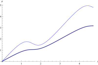
Figure 1. The phases $\theta_{0}\/\left(t\right)$ and $\theta_{1}\/\left(t\right)$ with $\alpha_{0}=\gamma_{0}=\varepsilon_{0}=0$, $\beta_{0}=2/3$ and $\delta_{0}=1$ (thick and thin lines, respectively).

Acknowledgments. We thank Michael Berry, Andrew Bremner, Carlos Castillo-Chávez, Victor V. Dodonov, Christoph Koutschan, Elliott Lieb, Francisco F. López-Ruiz, Vladimir I. Man’ko, Benjamin R. Morin, Sergey I. Kryuchkov, Andreas Ruffing, Vladimir M. Shabaev, Barbara Sanborn, Luc Vinet and Doron Zeilberger for support, valuable discussions and encouragement. This paper is written as a result of author’s visit to RISC, Research Institute for Symbolic Computation, and The Erwin Schrödinger International Institute for Mathematical Physics — we thank Peter Paule, RISC, Johannes Kepler Universität Linz, and Christian Krattenthaler, Fakultät für Mathematik, Universität Wien, for their hospitality. We are grateful to Catherine Boucher of Wolfram Science Group for an independent Mathematica verification of the “missing” solutions.

References

- [1] R. L. Anderson, S. Kumei and C. E. Wulfman, Invariants of the equations of wave mechanics. I, Rev. Mex. Fís. 21 (1972), 1–33.
- [2] R. L. Anderson, S. Kumei and C. E. Wulfman, Invariants of the equations of wave mechanics. II One-particle Schrödinger equations, Rev. Mex. Fís. 21 (1972), 35–57.
- [3] V. G. Bagrov, V. V. Belov and I. M. Ternov, Quasiclassical trajectory-coherent states of a particle in an arbitrary electromagnetic field, J. Math. Phys. 24 (1983) #12, 2855–2859.
- [4] V. V. Belov and A. G. Karavaev, Higher approximations for quasiclassical trajectory-coherent states, Izvestiya Vysshikh Uchebynkh Zavedenij Fizika, 31 (1987) #10, 14–18 [in Russian]; see also English transl.: Sov. Phys. Journal 1989, 30 #10, 819–822.
- [5] M. V. Berry, Quantal phase factors accompanying adiabatic changes, Proc. Roy. Soc. London, A392 (1984) # 1802, 45–57.
- [6] M. V. Berry, Classical adiabatic angles and quantum adiabatic phase, J. Phys. A: Math. Gen. 18 (1985) # 1, 15–27.
- [7] C. P. Boyer, R. T. Sharp and P. Winternitz, Symmetry breaking interactions for the time dependent Schrödinger equation, J. Math. Phys. 17 (1976) #8, 1439–1451.
- [8] R. Cordero-Soto, R. M. López, E. Suazo and S. K. Suslov, Propagator of a charged particle with a spin in uniform magnetic and perpendicular electric fields, Lett. Math. Phys. 84 (2008) #2–3, 159–178.
- [9] R. Cordero-Soto, E. Suazo and S. K. Suslov, Quantum integrals of motion for variable quadratic Hamiltonians, Ann. Phys. 325 (2010) #9, 1884–1912.
- [10] V. V. Dodonov, ‘Nonclassical’ states in quantum optics: a ‘squeezed’ review of the first 75 years, J. Opt. B: Quantum Semiclass. Opt. 4 (2002), R1–R33.
- [11] V. V. Dodonov, Current status of dynamical Casimir effect, Physica Scripta 82 (2010) #3, 038105 (10 pp).
- [12] V. V. Dodonov, A. B. Klimov and D. E. Nikonov, Quantum phenomena in nonstationary media, Phys. Rev. A. 47 (1993) # 5, 4422–4429.
- [13] V. V. Dodonov, I. A. Malkin and V. I. Man’ko, Integrals of motion, Green functions, and coherent states of dynamical systems, Int. J. Theor. Phys. 14 (1975) # 1, 37–54.
- [14] V. V. Dodonov and V. I. Man’ko, Coherent states and the resonance of a quantum damped oscillator, Phys. Rev. A 20 (1979) # 2, 550–560.
- [15] V. V. Dodonov and V. I. Man’ko, Invariants and correlated states of nonstationary quantum systems, in: Invariants and the Evolution of Nonstationary Quantum Systems, Proceedings of Lebedev Physics Institute, vol. 183, pp. 71-181, Nauka, Moscow, 1987 [in Russian]; English translation published by Nova Science, Commack, New York, 1989, pp. 103-261.
- [16] V. V. Dodonov and V. I. Man’ko, Adiabatic invariants, correlated states and Berry’s phase, in: Topological Phases in Quantum Theory, Proceedings of the International Seminar, Dubna, SU, September 1988 (B. Markovski and S. I. Vinitsky, Eds.), World Scientific, Singapore, 1989, pp. 74–83.
- [17] V. V. Dodonov and V. I. Man’ko, ‘Nonclassical’ states in quantum physics: brief historical review, in: Theory of Nonclassical States of Light, (V. V. Dodonov and V. I. Man’ko, Eds.), Taylor & Francis, London and New York, 2003, pp. 1–94.
- [18] S. Flügge, Practical Quantum Mechanics, Springer–Verlag, Berlin, 1999.
- [19] C. H. Hagen, Scale and conformal transformations in Galilean-covariant field theory, Phys. Rev. D 5 (1972) #2, 377–388.
- [20] S. W. Hawking, Black hole explosions?, Nature, London 248 (1974), 30–31.
- [21] S. W. Hawking, Particle creation by black holes, Commun. Math. Phys. 43 (1975) #3, 199–220.
- [22] K. Husimi, Miscellanea in elementary quantum mechanics: I–II, Prog. Theor. Phys. 9 (1953) #3, 238–244; Prog. Theor. Phys. 9 (1953) #4, 381–402.
- [23] R. Jackiw, Dynamical symmetry of the magnetic monopole, Ann. Phys. 129 (1980), 183–200.
- [24] T. A. Jacobson, Introduction to quantum fields in curved spacetime and the Hawking effect, arXiv:0308048v3 [gr-qc] 9 April 2004.
- [25] E. G. Kalnins and W. Miller, Lie theory and separation of variables. 5. The equations and J. Math. Phys. 15 (1974) #10, 1728–1737.
- [26] C. Koutschan, http://hahn.la.asu.edu/~suslov/curres/index.htm; see Mathematica notebook: Koutschan.nb; see also http://www.risc.jku.at/people/ckoutsch/pekeris/
- [27] P. Lähteenmäki, G. S. Paraoanu, J. Hassel and P. J. Hakonen, Dynamical Casimir effect in a Josephson metamaterial, arXiv:1111.5608v2 [cond-mat.mes-hall] 1 Dec 2011.
- [28] L. D. Landau and E. M. Lifshitz, Quantum Mechanics: Nonrelativistic Theory, Pergamon Press, Oxford, 1977.
- [29] N. Lanfear, R. M. López and S. K. Suslov, Exact wave functions for generalized harmonic oscillators, Journal of Russian Laser Research 32 (2011) #4, 352–361; see also arXiv:11002.5119v2 [math-ph] 20 Jul 2011.
- [30] R. M. López, S. K. Suslov and J. M. Vega-Guzmán, On the harmonic oscillator group, arXiv:1111.5569v2 [math-ph] 4 Dec 2011.
- [31] R. M. López, S. K. Suslov and J. M. Vega-Guzmán, http://hahn.la.asu.edu/~suslov/curres/index.htm; see Mathematica notebook: HarmonicOscillatorGroup.nb
- [32] R. M. López, S. K. Suslov and J. M. Vega-Guzmán, On a hidden symmetry of quantum harmonic oscillators, Journal of Difference Equations and Applications, 2012, http://dx.doi.org/10.1080/10236198.2012.658384; see also arXiv:1112.2586v2 [quant-ph] 2 Jan 2012.
- [33] I. A. Malkin and V. I. Man’ko, Dynamical Symmetries and Coherent States of Quantum System, Nauka, Moscow, 1979 [in Russian].
- [34] V. I. Man’ko, The Casimir effect and quantum vacuum generator, Journal of Soviet Laser Research 12 (1991), 383–385.
- [35] E. Merzbacher, Quantum Mechanics, third edition, John Wiley & Sons, New York, 1998.
- [36] W Miller, Jr., Symmetry and Separation of Variables, Encyclopedia of Mathematics and Its Applications, Vol. 4, Addison–Wesley Publishing Company, Reading etc, 1977.
- [37] P. D. Nation, J. R. Johansson, M. P. Blencowe and F. Nori, Stimulationg uncertainty: Amplifying the quantum vacuum with superconducting circuits, Rev. Mod. Phys. 84 (2012), January–March, 1–24.
- [38] U. Niederer, The maximal kinematical invariance group of the free Schrödinger equations, Helv. Phys. Acta 45 (1972), 802–810.
- [39] U. Niederer, The maximal kinematical invariance group of the harmonic oscillator, Helv. Phys. Acta 46 (1973), 191–200.
- [40] A. F. Nikiforov, S. K. Suslov, and V. B. Uvarov, Classical Orthogonal Polynomials of a Discrete Variable, Springer–Verlag, Berlin, New York, 1991.
- [41] B. Sanborn, S. K. Suslov and L. Vinet, Dynamic invariants and the Berry phase for generalized driven harmonic oscillators, Journal of Russian Laser Research 32 (2011) #5, 486–494; see also arXiv:1108.5144v1 [math-ph] 25 Aug 2011.
- [42] E. Schrödinger, Der stetige Übergang von der Mikro-zur Makro Mechanik, Die Naturwissenshaften, 14 (1926), 664–666; see also Collected Papers on Wave Mechnics, Blackie & Son Ltd, London and Glascow, 1928, pp. 41–44, for English translation of Schrödinger’s original paper.
- [43] B. Simon, Holonomy, the quantum adiabatic theorem, and Berry’s phase, Phys. Rev. Lett. 51 (1983) #24, 2167–2170.
- [44] S. K. Suslov, Dynamical invariants for variable quadratic Hamiltonians, Physica Scripta 81 (2010) #5, 055006 (11 pp); see also arXiv:1002.0144v6 [math-ph] 11 Mar 2010.
- [45] S. K. Suslov, http://hahn.la.asu.edu/~suslov/curres/index.htm; see Mathematica notebook: BerrySummary.nb.
- [46] D. Xiao, M.-Ch. Chang and Q. Niu, Berry phase effects on electronic properties, Rew. Mod. Phys. 82 (2010), July–September, 1959–2007.
- [47] W. G. Unruh, Notes on black-hole evaporation, Phys. Rev. D 14 (1976) #4, 870–892.
- [48] L. Vinet and A. Zhedanov, Representations of the Schrödinger group and matrix orthogonal polynomials, J. Phys. A: Math. Theor. 44 (2011) #35, 355201 (28 pages).
- [49] S. I. Vinitskiĭ, V. L.Derbov, V. N. Dubovik, B. L. Markovski, and Yu. P. Stepanovskiĭ, Topological phases in quantum mechanics and polarization optics, Sov. Phys. Usp. 33 (1990) #6, 403–428.
- [50] F. Wilczek and A. Zee, Appearance of gauge structure in simple dynamical systems, Phys. Rev. Lett. 52 (1984) #24, 2111–2114.
- [51] C. M. Wilson, G. Johansson, A. Pourkabirian, M. Simoen, J. R. Johansson, T. Duty, F. Nori and P. Delsing, Observation of the dynamical Casimir effect in a superconducting circuit, Nature 479 (2011) November 17, 376–379.
- [52] K. B. Wolf, On time-dependent quadratic Hamiltonians, SIAM J. Appl. Math. 40 (1981) #3, 419–431.
- [53] K-H. Yeon, K-K. Lee, Ch-I. Um, T. F. George and L. N. Pandey, Exact quantum theory of a time-dependent bound Hamiltonian systems, Phys. Rev. A 48 (1993) # 4, 2716–2720.