Medium Access Control Protocols for Wireless Sensor Networks with Energy Harvesting

Abstract

The design of Medium Access Control (MAC) protocols for wireless sensor networks (WSNs) has been conventionally tackled by assuming battery-powered devices and by adopting the network lifetime as the main performance criterion. While WSNs operated by energy-harvesting (EH) devices are not limited by network lifetime, they pose new design challenges due to the uncertain amount of harvestable energy. Novel design criteria are thus required to capture the trade-offs between the potentially infinite network lifetime and the uncertain energy availability.

This paper addresses the analysis and design of WSNs with EH devices by focusing on conventional MAC protocols, namely TDMA, Framed-ALOHA (FA) and Dynamic-FA (DFA), and by accounting for the performance trade-offs and design issues arising due to EH. A novel metric, referred to as delivery probability, is introduced to measure the capability of a MAC protocol to deliver the measure of any sensor in the network to the intended destination (or fusion center, FC). The interplay between delivery efficiency and time efficiency (i.e., the data collection rate at the FC), is investigated analytically using Markov models. Numerical results validate the analysis and emphasize the critical importance of accounting for both delivery probability and time efficiency in the design of EH-WSNs.

I Introduction

Recent advances in low-power electronics and energy-harvesting (EH) technologies enable the design of self-sustained devices that collect part, or all, of the needed energy from the surrounding environment. Several systems can take advantage of EH technologies, ranging from portable devices to wireless sensor networks (WSNs) [1]. However, EH devices open new design issues that are different from conventional battery-powered (BP) systems [2], where the main concern is the network lifetime [3]. In fact, EH potentially allows for perpetual operation of the network, but it might not guarantee short-term activities due to temporary energy shortages [2]. This calls for the development of energy management techniques tailored to the EH dynamics. While such techniques have been mostly studied at a single-device level [4], in wireless scenarios where multiple EH devices interact with each other, the design of EH-aware solutions needs to account for a system-level approach [5][6]. This is the motivation of this work.

In this paper, we focus on system-level design considerations for WSNs operated by EH-capable devices. In particular, we address the analysis and design of medium access control (MAC) protocols for single-hop WSNs (see Fig. 1) where a fusion center (FC) collects data from sensors in its surrounding. Specifically, we investigate how performance and design of MAC protocols routinely used in WSNs, such as TDMA [7], Framed-ALOHA (FA) and Dynamic-FA (DFA) [8], are influenced by the discontinuous energy availability in EH-powered devices.

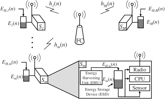
Figure 1: WSN with a single Fusion Center (FC) gathering data from $M$ sensors, which are equipped with an energy storage device (ESD) and an energy-harvesting unit (EHU).

I-A State of the Art

In recent years, WSNs with EH-capable nodes have been attracting a lot of attention, also at commercial level. To provide some examples, the Enocean Alliance proposes to use a MAC protocol for EH devices based on pure ALOHA strategies [11], while an enhanced self-powered RFID tag created by Intel, referred to as WISP [12], has been conceived to work with the EPC Gen 2 standard [13] that adopts a FA-like MAC protocol.

However, while performance analysis of MAC protocols in BP-WSNs have been investigated in depth (see e.g., [7][8][14]), analyses of MAC protocols with EH are hardly available. A notable exception is [6], where data queue stability has been studied for TDMA and carrier sense multiple access (CSMA) protocols in EH networks. We remark that routing for EH networks has instead received more attention, see e.g., [2][15].

I-B Contributions

In this paper we consider the design and analysis of TDMA, FA and DFA MAC protocols in the light of the novel challenges introduced by EH. In Sec. III we propose to measure the system performance in terms of the trade-off between the delivery probability, which accounts for the number of sensors’ measurements successfully reported to the FC, and the time efficiency, which measures the rate of data collection at the FC (formal definitions are in Sec. III). We then introduce an analytical framework in Sec. IV and Sec. V to assess the performance of EH-WSNs in terms of the mentioned trade-off for TDMA, FA and DFA MAC protocols. In Sec. VI we tackle the critical issue in ALOHA-based MAC protocols of estimating the number of EH sensors involved in transmission, referred to as backlog, by proposing a practical reduced-complexity algorithm. Finally, we present extensive numerical simulations in Sec. VII to get insights into the MAC protocol design trade-offs, and to validate the analytical derivations.

II System Model

In this paper, we consider a single-hop WSN with a FC surrounded by $M$ wireless sensors labeled as $S_{1},S_{2},...,S_{M}$ (see Fig. 1). Each sensor (or user) is equipped with an EH unit (EHU) and an energy storage device (ESD), where the latter is used to store the energy harvested by the EHU. The FC retrieves measurements from sensors via periodic inventory rounds (IRs), once every $T_{int}$ seconds $[s]$. Each IR is started by the FC by transmitting an initial query command (Q), which provides both synchronization and instructions to sensors on how to access the channel. Time is slotted, with each slot lasting $T_{s}$ $[\mathrm{s}]$. The effective duration of the $n$th IR, during which communication between the FC and the sensors takes place, is denoted by $T_{IR}(n)$. We assume that $T_{IR}(n)\ll T_{int}$ for all IR $n$, and also that the query duration is negligible, so that the ratio $T_{IR}(n)/T_{s}$ indicates the total number of slots allocated by the FC during the $n$th IR.

In every IR, each sensor has a new measure to transmit with probability $\alpha$, independently of other sensors and previous IRs. If a new measure is available, the sensor will mandatory attempt to report it successfully to the FC as long as enough energy is stored in its ESD (see Sec. II-B for details). Each measure is the payload of a packet, whose transmission fits within the slot duration $T_{s}$. Sensors’ transmissions within each IR are organized into frames, each of which is composed of a number of slots that is selected by the FC. Depending on the adopted MAC protocol, any user that needs to (and can) transmit in a frame either chooses or is assigned a single slot within the frame for transmission as it will be detailed below. Moreover, after a user has successfully transmitted its packet to the FC, it first receives an acknowledge (ACK) of negligible duration by the FC and then it becomes inactive for the remaining of the IR. We emphasize that the FC knows neither the number of sensors with a new measure to transmit, nor the state of sensors’ ESDs.

II-A Interference Model

We consider interference-limited communication scenarios where the downlink packets transmitted by the FC are always correctly received (error-free) by the sensors, while uplink packets transmitted by the sensors to the FC are subject to communication errors due to possible interference arising from collisions with other transmitting sensors. The uplink channel power gain for the $m$th sensor during the $n$th IR is $h_{m}(n)$. Channel gain $h_{m}(n)$ is assumed to be constant over the entire IR but subject to random independent and identically distributed (i.i.d.) fading across IRs and sensors, with pdf $f_{h}(\cdot)$ and normalized such that $E\left[h_{m}(n)\right]=1$, for all $n,m$. In the presence of simultaneous transmissions within the same slot during the $k$th frame of the $n$th IR, a sensor, say $S_{m}$, is correctly received by the FC if and only if its instantaneous signal-to-interference ratio (SIR) $\gamma_{m,k}\left(n\right)$ is larger than a given threshold $\gamma_{th}$, i.e., if

$$\gamma_{m,k}\left(n\right)=\frac{h_{m}\left(n\right)}{\sum_{l\in\mathcal{I}_{m,k}(n)}h_{l}\left(n\right)}\geq\gamma_{th},$$ (1)

where $\mathcal{I}_{m,k}(n)$ denotes the set of sensors that transmit in the same slot selected by $S_{m}$ in frame $k$ and IR $n$. We assume $\gamma_{th}>0dB$ so that, in case a slot is selected by more than one sensor, at most one of the colliding sensor can be successfully decoded in the slot.

According to the interference model (1), any slot can be: empty when it is not selected by any sensor; collided when it is chosen by more than one sensors but none of them transmits successfully; successful when one sensor transmits successfully possibly in the presence of other (interfering) users. Successful transmission in the presence of interfering users within the same slot is often referred to as capture effect [14].

Remark 1: Errors in the decoding of downlink query packets can be accounted for through the parameter $\alpha$ as well. In fact, let $\alpha_{Q}$ be the probability that a user correctly decodes the downlink packet sent by the FC at the beginning of an IR. Moreover, assume that downlink decoding errors are i.i.d. across sensors and IRs, and let $\alpha_{N}$ be the probability that a user has a new measure to transmit in any IR. Then, the probability that any user $S_{m}$ has a new measure and correctly decodes the FC’s query is given by the product $\alpha=\alpha_{Q}\alpha_{N}$.

II-B ESD and Energy Consumption Models

We consider a discrete ESD with $N+1$ energy levels in the set $\mathcal{E}=\{0,\mathcal{\delta},2\mathcal{\delta},...,N\mathcal{\delta}\}$, where $\mathcal{\delta}$ is referred to as energy unit. Let $E_{m}(n)\in\mathcal{E}$ be the energy stored in the ESD of the $m$th user at the beginning of the $n$th IR. Energy $E_{m}(n)$ is a random variable that is the result of the EH process and the energy consumption of the sensor across IRs; its probability mass function (pmf) is $p_{E(n)}\left(\cdot\right)$ and the corresponding complementary cumulative distribution function (ccdf) is $G_{E(n)}\left(x\right)=\Pr[E_{m}(n)\geq x]$. Note that, the initial energy distribution $p_{E(1)}\left(\cdot\right)$ is given, while the evolution of the pmf $p_{E(n)}\left(\cdot\right)$ for $n>1$ depends on both the MAC protocol and EH process.

We assume that each time a sensor transmits a packet it consumes an energy $\varepsilon$, which accounts for the energy consumed in the: a) reception of the FC’s query that starts the frame (see Fig. 2); b) transmission; c) reception of FC’s ACK or not ACK (NACK) packet. At the beginning of each IR, a sensor with a new measure to transmit can participate to the current IR only if the energy stored in its ESD is at least $\varepsilon$. Let $\varepsilon_{\mathcal{\delta}}=\varepsilon/\mathcal{\delta}$ be the number of energy units $\mathcal{\delta}$ required for transmission, where $\varepsilon_{\mathcal{\delta}}$ is assumed to be an integer value without loss of generality. Let $F_{\varepsilon}=N\mathcal{\delta}/\varepsilon=N/\varepsilon_{\mathcal{\delta}}$ be the (normalized) capacity of the ESD, which is assumed to be an integer indicating the maximum number of (re)transmissions allowed by a fully charged ESD.

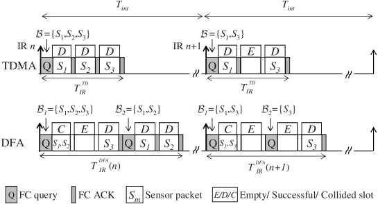
Figure 2: Examples for TDMA and DFA MAC protocols for $M=3$. FA is not depicted since it is a special case of DFA with only one frame. The backlog for each frame is indicated above each query. Some sensors might not be in the backlog due to energy shortage and/or absence of a new measure to report.

II-C Energy Harvesting Model

During the time $T_{int}$ between the $n$th and $(n+1)$th IRs the $m$th sensor $S_{m}$ harvests an energy $E_{H,m}(n)$, which is modeled as a discrete random variable, i.i.d. over IRs and sensors, with pmf $q_{i}=\Pr[E_{H,m}(n)=i\mathcal{\delta}]$, with $i\in\{0,1,2,...\}$, and for all $m$ and $n$. For technical reasons that we discuss in Sec. V-B, we assume that the probability $q_{0}$ and $q_{1}$ of harvesting zero and one energy unit respectively, are both strictly positive, namely $q_{0}>0$ and $q_{1}>0$.

We assume that the EH dynamics is much slower than the IR duration $T_{IR}(n)$, so that the amount of energy harvested within $T_{IR}(n)$ can be considered as negligible with respect to $\varepsilon$ (recall also that $T_{IR}(n)\ll T_{int}$). Hence, the only energy that a sensor can actually use throughout an IR is the energy initially available at the beginning of the IR itself (i.e., $E_{m}(n)$).

III Performance Metrics and Medium Access Control Protocols

We first introduce in Sec. III-A the considered performance metrics, namely delivery probability and time efficiency, and then in Sec. III-B we review the considered MAC protocols.

III-A MAC Performance Metrics

III-A1 Delivery Probability

The delivery probability $p_{d}\left(n\right)$ measures the capability of the MAC protocol to successfully deliver the measure of any sensor, say $S_{m}$, to the FC during the $n$th IR

$$p_{d}(n)=\Pr\left[S_{m}\text{ transmits successfully in IR }n|\text{ }S_{m}\text{ has a new measure in IR }n\right].$$ (2)

The statistical equivalence of all sensors makes the probability (2) independent of the specific sensor. Notice that a sensor fails to report its measure during an IR if either it has an energy shortage before (re)transmitting the packet correctly, or the MAC protocol does not provide the sensor with sufficient retransmission opportunities. Given the potentially perpetual operation enabled by EH, it is relevant to evaluate the delivery probability when the system is in steady-state. The asymptotic delivery probability is thus obtained by taking the limit of $p_{d}\left(n\right)$ for large IR index $n$, provided that it exists, as

$$p_{d}^{AS}=\underset{n\rightarrow\infty}{\lim}p_{d}(n).$$ (3)

III-A2 Time Efficiency

The time efficiency $p_{t}(n)$ measures the probability that any slot allocated by the MAC within the $n$th IR is successfully used (i.e., it is neither empty nor collided, see Sec. II-A)

$$p_{t}\left(n\right)=\Pr\left[\text{The FC correctly retrieves a packet in any slot of the }n\text{th IR}\right].$$ (4)

By taking the limit of (4) for $n\rightarrow\infty$, we obtain the asymptotic time efficiency

$$p_{t}^{AS}=\underset{n\rightarrow\infty}{\lim}p_{t}\left(n\right).$$ (5)

Remark 2: Informally speaking, the time efficiency $p_{t}(n)$ measures the ratio between the total number of packets successfully received by the FC and the total number of slots allocated by the MAC protocol (i.e., $T_{IR}(n)/T_{s}$, see Sec. II). As it will be shown in Sec. III-B, the IR duration $T_{IR}(n)$ is in general a random variable, and consequently, time efficiency $p_{t}(n)$ differs from more conventional definitions of throughput (see e.g., [8]) which measure the number of packets delivered over the interval between two successive IRs $T_{int}$, instead of $T_{IR}(n)$. The rationale for this definition of time efficiency is that it actually captures more effectively the rate of data collection at the FC. Whereas, the delivery probability accounts for the fraction of users, with a new measure to transmit at the beginning of the current IR, which are able to successfully report their payload to the FC within the IR, where delivery failures are due to collisions and energy shortages.

In contention based MACs (e.g., ALOHA), there is a trade-off between delivery probability and time efficiency. In fact, increasing the former generally requires the FC to allocate a larger number of slots in an IR to reduce packet collisions, which in turn decreases the time efficiency.

III-B MAC Protocols

In this section, we review the standard MAC protocols that we focus on.

III-B1 TDMA

With the TDMA protocol, each user is pre-assigned an exclusive slot that it can use in every IR, irrespective of whether it has a measure to deliver or enough energy to transmit. Recall that such information is indeed not available at the FC. Every $n$th IR is thus composed by one frame with $M$ slots and has fixed duration $T_{IR}^{TD}=MT_{s}$, as shown in Fig. 2. Since TDMA is free of communication errors in the considered interference-limited scenario, its delivery probability $p_{d}(n)$ is only limited by energy availability and it is thus an upper bound for ALOHA-based MACs. However, TDMA might not be time efficient due to the many empty slots when the probability of having a new measure $\alpha$ and/or the EH rate are small.

III-B2 Framed-ALOHA (FA) and Dynamic-FA (DFA)

Hereafter we describe the DFA protocol only, since FA follows as a special case of DFA with no retransmissions capabilities as discussed below. The $n$th IR, of duration $T_{IR}^{DFA}(n)$, is organized into a set of frames as shown in Fig. 2. The backlog $\mathcal{B}_{k}(n)$ for the $k$th frame is the set composed of all sensors that simultaneously satisfy the following three conditions: i) have a new measure to transmit in the $n$th IR; ii) have transmitted unsuccessfully (because of collisions) in the previous $k-1$ frames (this condition does not apply for frame $k=1$); iii) have enough energy left in the ESD to transmit in the $k$th frame. All the users in the set $\mathcal{B}_{k}(n)$, whose cardinality $\left|\mathcal{B}_{k}(n)\right|=B_{k}(n)$ is referred to as backlog size, thus attempt transmission during frame $k$. To make this possible, the FC allocates a frame of $L_{k}(n)$ slots, where $L_{k}(n)$ is selected based on the estimate $\hat{B}_{k}(n)$ of the backlog size $B_{k}(n)$ (estimation of $B_{k}(n)$ is discussed in Sec. VI) as

$$L_{k}(n)=\left\lceil\rho\hat{B}_{k}(n)\right\rceil,$$ (6)

where $\left\lceil\cdot\right\rceil$ is the upper nearest integer operator, and $\rho$ is a design parameter. Note that, if the backlog size is $B$, the probability $\beta\left(j,B,L\right)$ that $j\leq B$ sensors transmit in the same slot in a frame of length $L$ is binomial [16]

$$\beta\left(j,B,L\right)=\binom{B}{j}\left(\frac{1}{L}\right)^{j}\left(1-\frac{1}{L}\right)^{B-j}.$$ (7)

Finally, FA is a special case of DFA where only one single frame of size $L_{1}(n)$ is announced as retransmissions are not allowed within the same IR.

IV Analysis of the MAC Performance Metrics

In this section we derive the performance metrics defined in Sec. III-A for TDMA, FA and DFA. The analysis is based on two simplifying assumptions:

• Known backlog: the FC knows the backlog size $B_{k}(n)=\left|\mathcal{B}_{k}(n)\right|$ before each $k$th frame;

• Large backlog: the backlog size $B_{k}(n)$, in any IR $n$ and any frame $k$ of size $L_{k}(n)=\left\lceil\rho B_{k}(n)\right\rceil$, is large enough to let the probability (7) be approximated by the Poisson distribution [16]:

$$\beta\left(j,B_{k}(n),L_{k}(n)\right)\simeq\frac{e^{-\frac{1}{\rho}}}{\rho^{j}j!}.$$ (8)

Assumption $\mathcal{A}.1$ simplifies the analysis as in reality the backlog can only be estimated by the FC (see Sec. VI and Sec. VII for the impact of backlog estimation). Assumption $\mathcal{A}.2$ is standard and analytically convenient, as it makes the probability $\beta\left(j,B_{k}(n),L_{k}(n)\right)$ dependent only on the ratio $\rho$ between the frame length $L_{k}(n)$ and the backlog size $B_{k}(n)$. The assumptions above are validated numerically in Sec. VII.

IV-A Delivery Probabilities

Here we derive the delivery probability (2) within any $n$th IR under the assumptions $\mathcal{A}.1$ and $\mathcal{A}.2$ for the considered MAC protocols. The IR index $n$ is dropped to simplify the notation.

IV-A1 Delivery Probability for TDMA

As the TDMA protocol is free of collisions, each sensor $S_{m}$ that has a new measure to report in the current IR cannot deliver its payload to the FC only when it is in energy shortage, namely if $E_{m}<\varepsilon$. Provided that user $S_{m}$ has a new measure to transmit, the delivery probability (2) reduces to

$$p_{d}^{TD}=\Pr\left[E_{m}\geq\varepsilon\right]=G_{E}^{TD}\left(\varepsilon\right),$$ (9)

which is independent of the sensor index $m$ and dependent only on the ccdf $G_{E}^{TD}\left(\cdot\right)$ of the energy stored in sensor ESD at the beginning of the considered IR. The ESD energy distribution for any arbitrary $n$th IR is derived in Sec. V.

IV-A2 Delivery Probability for FA

In the FA protocol, each sensor $S_{m}$ that has a new measure to report in the current IR is able to correctly deliver its payload to the FC only if: a) it transmits successfully in the selected slot, possibly in the presence of interfering users provided that its SIR is $\gamma_{m,1}\geq\gamma_{th}$; and b) it has enough energy to transmit. From (1), the probability that sensor $S_{m}$, with $S_{m}\in\mathcal{B}_{1}$, transmits successfully in the selected slot, given that $\left|\mathcal{I}_{m,1}\right|=j$ users select the same slot of $S_{m}$ (thus colliding), is given by

$$p_{c}(j)=\Pr\left[h_{m}\geq\gamma_{th}\sum_{l=1}^{j}h_{l}\right],$$ (10)

where, without loss of generality, we assumed that $\mathcal{I}_{m,1}=\{S_{1},...,S_{j}\}$, and $S_{m}\notin\mathcal{I}_{m,1}$, as users are stochastically equivalent. Under the large backlog assumption $\mathcal{A}.2$, the probability that there are $j$ interfering users is Poisson-distributed (see (8)), and thus the unconditional probability $p_{c}$ that $S_{m}$ captures the selected slot can be approximated as

$$p_{c}\simeq e^{-\frac{1}{\rho}}\sum_{j=0}^{\infty}\frac{1}{\rho^{j}j!}p_{c}(j).$$ (11)

Note that, in (11) we also extended the number of possible interfering users up to infinity as $p_{c}(j)$ rapidly vanishes for increasing $j$. Moreover, depending on the channel gain pdf $f_{h}(\cdot)$, probabilities (10) can be calculated either analytically (e.g., when $f_{h}(\cdot)$ is exponential, see [17]) or numerically.

Finally, under assumption $\mathcal{A}.2$, the successful transmission event is independent of the ESD energy levels (which in principle determine the actual backlog size in (7)), and thus the delivery probability (2) for the FA protocol can be calculated as the product between the probability $G_{E}^{FA}\left(\varepsilon\right)=\Pr\left[E_{m}\geq\varepsilon\right]$ that sensor $S_{m}$ has enough energy to transmit and the (approximated) capture probability (11) as

$$p_{d}^{FA}\simeq G_{E}^{FA}\left(\varepsilon\right)e^{-\frac{1}{\rho}}\sum_{j=0}^{\infty}\frac{1}{\rho^{j}j!}p_{c}(j),$$ (12)

where the ESD energy ccdf $G_{E}^{FA}\left(\varepsilon\right)$ for any arbitrary $n$th IR is derived in Sec. V.

IV-A3 Delivery Probability for DFA

DFA is composed of several instances of FA, one for each $k$th frame of the current IR. As DFA allows retransmissions, we need to calculate the probability $p_{c,k}(j)$ that any sensor active during frame $k$, say $S_{m}\in\mathcal{B}_{k}$, transmits successfully in the selected slot given that there are $\left|\mathcal{I}_{m,k}\right|=j$ users that transmit in the same slot, with $\mathcal{I}_{m,k}\subseteq\mathcal{B}_{k}$. The computation of $p_{c,k}(j)$, for $k>1$, is more involved than (10). In fact, packets collisions introduce correlation among the channel gains of collided users, as any sensor in the backlog $\mathcal{B}_{k}$, for $k>1$, might have collided with some other sensors in the set $\mathcal{B}_{k}$. We recall that, even though the channel gains are i.i.d. at the beginning of the IR, they remain fixed for the entire IR.

While the exact computation of probabilities $p_{c,k}(j)$ is generally cumbersome, the large backlog assumption $\mathcal{A}.2$ enables some simplifications. Specifically, correlation among channel gains can be neglected, since for large backlogs it is unlikely that two users collide more than once within the same IR. By assuming independence among the channel gains at any frame, calculation of $p_{c,k}(j)$ requires only to evaluate the channel gain pdf $f_{h}^{(k)}(\cdot)$ at the $k$th frame for any user within $\mathcal{B}_{k}$, which is the same for all users by symmetry. The computation of pdf $f_{h}^{(k)}(\cdot)$ can be done recursively, starting from frame $k=1$, so that at frame $k$ we condition on the event that the SIR (1) was $\gamma_{m,k-1}<\gamma_{th}$. Under assumption $\mathcal{A}.2$, this can be done numerically.

Now, let $\tilde{h}_{m}^{(k)}$, for $m\in\{1,...,M\}$ and $k\in\{1,...,F_{\varepsilon}\}$, be random variables with pdf $f_{h}^{(k)}(\cdot)$ independent over $m$, where $\tilde{h}_{m}^{(1)}=h_{m}$. The conditional capture probabilities $p_{c,k}(j)$ can then be approximated as (compare to (10))

$$p_{c,k}(j)\simeq\Pr\left[\tilde{h}_{m}^{(k)}\geq\gamma_{th}\sum_{l=1}^{j}\tilde{h}_{l}^{(k)}\right],$$ (13)

for any $m\notin\{1,...,j\}$ as users are stochastically equivalent. By exploiting the Poisson approximation similarly to (11), the unconditional probability that any user within the backlog successfully transmits in the selected slot during the $k$th frame becomes

$$p_{c,k}\simeq e^{-\frac{1}{\rho}}\sum_{j=0}^{\infty}\frac{1}{\rho^{j}j!}p_{c,k}(j).$$ (14)

Recalling that a user keeps retransmitting its message until it is successfully delivered to the FC, then the successful delivery of a message in a frame is a mutually exclusive event with respect to the delivery in previous frames. Therefore, the probability of transmitting successfully in the $k$th frame, given that enough energy is available, is $p_{c,k}\prod_{i=1}^{k-1}\left(1-p_{c,i}\right).$ Finally, by accounting for the probability $G_{E}^{DFA}\left(k\varepsilon\right)=\Pr\left[E_{m}\geq k\varepsilon\right]$ of having enough energy in each $k$th frame, the DFA delivery probability can be obtained, under assumption $\mathcal{A}.2$, as

$$p_{d}^{DFA}\simeq\sum_{k=1}^{F_{\varepsilon}}G_{E}^{DFA}\left(k\varepsilon\right)p_{c,k}\prod_{i=1}^{k-1}\left(1-p_{c,i}\right),$$ (15)

where the ESD energy ccdf $G_{E}^{DFA}\left(k\varepsilon\right)$ for any arbitrary $n$th IR is derived in Sec. V.

IV-B Time Efficiencies

In this section we derive the time efficiency (4) for the three considered protocols.

IV-B1 Time Efficiency for TDMA

Let $\mathcal{M}_{m}$ be the event indicating that user $S_{m}$ has a new measure to report in the current IR, with $\Pr[\mathcal{M}_{m}]=\alpha$, then the TDMA time efficiency (4) is given by the probability that the $m$th user has enough energy to transmit and a new measure to report:

$$p_{t}^{TD}=\Pr\left[E_{m}\geq\varepsilon,\mathcal{M}_{m}\right]=\Pr\left[E_{m}\geq\varepsilon\right]\Pr\left[\mathcal{M}_{m}\right]=\alpha G_{E}^{TD}\left(\varepsilon\right),$$ (16)

where we exploited independence between energy availability $E_{m}$ and $\mathcal{M}_{m}$.

IV-B2 Time Efficiency for FA

Since we assumed $\gamma_{th}>0dB$, then when more than one user transmits within the same slot, only one of them can be decoded successfully, that is, successful transmissions of different users within the same slot are disjoint events. Therefore, the probability that a slot, simultaneously selected by $j$ users, is successfully used by any of them is given by $jp_{c}(j-1)$, where $p_{c}(j-1)$ is (10) by recalling that any user have $(j-1)$ interfering users. Furthermore, under assumption $\mathcal{A}.2$, the probability that exactly $j$ users select the same slot is $e^{-\frac{1}{\rho}}/\left(\rho^{j}j!\right)$, and by summing up over the number of simultaneously transmitting users $j$ we get

$$p_{t}^{FA}\simeq e^{-\frac{1}{\rho}}\sum_{j=1}^{\infty}\frac{1}{\rho^{j}j!}jp_{c}(j-1)=e^{-\frac{1}{\rho}}\sum_{j=0}^{\infty}\frac{1}{\rho^{(j+1)}j!}p_{c}\left(j\right)$$ (17)

Note that, a consequence of assumption $\mathcal{A}.2$ is to make the FA time efficiency (17) independent of the ESD energy distribution. Moreover we remark that, when $\rho=1$, $p_{c}(j)=1$ for $j=0$ and $p_{c}(j)=0$ for $j>0$, then we have $p_{t}^{FA}=e^{-1}$, which is the throughput of slotted ALOHA [8].

IV-B3 Time Efficiency for DFA

The derivation of the DFA time efficiency $p_{t}^{DFA}$ follows from the FA time efficiency by accounting for the presence of multiple frames within an IR similarly to Sec. IV-A3. Since the time efficiency is defined over multiple frames, we first derive the time efficiency in the $k$th frame, similarly to (17) but considering (13) instead of (10), as

$$p_{t,k}^{DFA}\simeq e^{-\frac{1}{\rho}}\sum_{j=0}^{\infty}\frac{1}{\rho^{(j+1)}j!}p_{c,k}\left(j\right).$$ (18)

We then calculate $p_{t}^{DFA}$ by summing (18) up, for all $k\in\{1,...,F_{\varepsilon}\}$, weighted by the (random) length of the corresponding frame $L_{k}$ normalized to the total number of slots in the IR $\sum_{k=1}^{F_{\varepsilon}}L_{k}$. Note that, under assumption $\mathcal{A}.2$ the random frame length $L_{k}$ is well-represented by its (deterministic) average value $L_{k}\simeq E\left[L_{k}\right]=\rho E\left[B_{k}\right]$ and thus the DFA time efficiency results

$$p_{t}^{DFA}\simeq\frac{\sum_{k=1}^{F_{\varepsilon}}p_{t,k}^{DFA}E\left[B_{k}\right]}{\sum_{k=1}^{F_{\varepsilon}}E\left[B_{k}\right]},$$ (19)

where the average backlog size $E[B_{k}]$ in frame $k$, can be computed, under assumption $\mathcal{A}.2$, as $E[B_{k}]=M\alpha G_{E}^{DFA}(k\varepsilon)\prod_{i=1}^{k-1}\left(1-p_{c,i}\right)$. In fact, $M\alpha$ indicates the average number of users that have a new measure to report in the current IR, $G(k\varepsilon)$ is the probability that $k\varepsilon$ energy units are stored in the ESD at the beginning of the IR, thus allowing $k$ successful transmissions, and $\prod_{i=1}^{k-1}\left(1-p_{c,i}\right)$ is the probability that a sensor collides in all of the first $(k-1)$ frames.

V ESD energy evolution

In Sec. IV we have shown that the performance metrics for the $n$th IR depend on the energy distribution in the sensor ESD at the beginning of the IR itself. The goal of this section is to derive the ccdf $G_{E(n)}(\cdot)$, for any IR $n$, in order to obtain the asymptotic performance metrics (3) and (5) from Sec. IV-A and Sec. IV-B respectively.

In general, the evolution of sensor ESDs across IRs in DFA are correlated with each other, due to the possibility of retransmitting after collisions. However, under the large backlog assumption $\mathcal{A}.2$, similarly to the discussion in Sec. IV-A3, the evolution of sensor ESDs become decoupled and can thus be studied separately. Accordingly, we develop a stochastic model, based on a discrete Markov chain (DMC) that focuses on a single sensor ESD as shown in Fig. 3. In addition, we concentrate on the DFA protocol as ESD evolutions for TDMA and FA follow as special cases. Note that, in TDMA (or FA), the evolution of sensor ESDs are actually independent with each other as retransmissions are not required (or allowed).

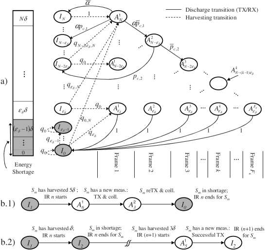
Figure 3: a) Discrete Markov chain used to model the evolution of the energy stored in the discrete ESD of a sensor in terms of the energy unit $\delta$. In b.1) and b.2) there are two outcomes of possible state transition chains for $\varepsilon_{\delta}=3$. Grey shaded states indicate energy shortage condition. Some transitions are not depicted to simplify representation. ($\bar{\alpha}=1-\alpha$ and $\bar{p}_{c,k}=1-p_{c,k}$).

V-A States of a Sensor

The state of a sensor is uniquely characterized by: i) sensor activity or idleness (see below); ii) the amount of energy stored in its ESD; iii) the current frame index if the sensor is active. A sensor is active if it has a new measure still to be delivered to the FC in the current IR and enough energy in its ESD, while it is idle otherwise. States in which the sensor is active, referred to as active states, are denoted by $A_{j}^{k}$ and they are characterized by: a) the current frame index $k\in\{1,...,F_{\varepsilon}\}$; and b) the number $j\in\{0,...,N\}$ of energy units $\delta$ stored in the sensor ESD.

States in which the sensor is idle, referred to as idle states, are instead denoted by $I_{j}$ and they are uniquely characterized by the number $j\in\{0,...,N\}$ of energy units stored in the sensor ESD. EH is then associated to idle states given the assumption that any energy arrival in the current IR can only be used in the next IR (see Sec. II-C).

V-B Discrete Markov Chain (DMC) Model

Operations of a sensor across IRs are as follows. When sensor $S_{m}$ is not involved in an IR, it is in an idle state, say $I_{j}$, waiting for the next IR. When a new IR begins, the energy harvested in the last interval $T_{int}$ is added, so that, if the ESD is not in energy shortage, the state makes a transition $I_{j}$ $\rightarrow A_{l}^{1}$ toward an active state, with $l\geq\varepsilon_{\mathcal{\delta}}\geq j$. Otherwise, if it is in energy shortage, it makes a transition $I_{j}\rightarrow I_{l}$ toward another idle state, with $j\leq l<\varepsilon_{\mathcal{\delta}}$. If sensor $S_{m}$ is not in energy shortage, it remains in state $A_{j}^{1}$ at the beginning of the IR only if it has a new measure to transmit, which happens with probability $\alpha$. Instead, with probability $\bar{\alpha}=1-\alpha$ the state makes a transition toward an idle state as $A_{j}^{1}\rightarrow I_{j}$. If there is a new measure, the sensor keeps transmitting it in successive frames until either the packet is correctly delivered to the FC, or its ESD falls in energy shortage, or both. A collision in frame $k$ happens with probability $\bar{p}_{c,k}=1-p_{c,k}$ (see Sec. IV-A3) and leads to a transition either $A_{j}^{k}\rightarrow A_{j-\varepsilon_{\mathcal{\delta}}}^{k+1}$, for $j\geq 2\varepsilon_{\mathcal{\delta}}$ (no shortage after collision) or $A_{j}^{k}\rightarrow I_{j-\varepsilon_{\mathcal{\delta}}}$, for $j<2\varepsilon_{\mathcal{\delta}}$ (shortage after collision). Successful transmissions in frame $k$, which happens with probability $p_{c,k}$, instead leads to a transition $A_{j}^{k}\rightarrow I_{j-\varepsilon_{\mathcal{\delta}}}$. Transition probabilities are summarized in Fig. 4, where we have defined $q_{j,N}=\Pr[E_{H,m}\geq(N-j)\mathcal{\delta}]=1-\sum_{i=0}^{N-j-1}q_{i}$. Note that, the probability $\alpha$ of having a new measure is only accounted for in active states in the first frame (i.e., in states $A_{j}^{1}$, for $j\in\{0,...,N\}$, see Fig. 4-b)). In fact, being in any state $A_{j}^{k}$ for $k>1$ already implies that a new measure was available at the beginning of the IR. Notice that, according to the model above, state transitions in the DMC at hand are event-driven and do not happen at fixed time intervals. A sketch of the considered DMC is shown in Fig. 3-a), while we show two outcomes of possible state transition chains in Fig. 3-b.1) and 3-b.2).

From Fig. 3-a), it can be seen that, when $q_{0}>0$, $q_{1}>0$ and $p_{c,k}>0$, for $k\in\{1,...,F_{\varepsilon}\}$, the DMC at hand is irreducible and aperiodic and thus, by definition, ergodic (see [18]). In fact, if $q_{1}>0$, any state of the Markov model can be reached from any other state with non-zero probability, and therefore the Markov chain is irreducible. Moreover, the probability of having a self-transition from state $I_{0}$ to itself is $q_{0}>0,$ and therefore state $I_{0}$ is aperiodic. The presence of an aperiodic state in a finite state irreducible Markov chain is enough to conclude that the chain is aperiodic [18, Ch. 4, Th. 1]. Since the DMC is ergodic it admits a unique steady-state probability distribution $\mathbf{\phi=[}\phi_{I_{0}},...,\phi_{I_{N}},\phi_{A_{\varepsilon_{\mathcal{\delta}}}^{1}},...,\phi_{A_{N}^{F_{\varepsilon}}}]$, regardless of the initial distribution, which can be calculated by resorting to conventional techniques [18]. This also guarantees the existence of limits (3) and (5). Vector $\mathbf{\phi}$ represents the steady-state distribution in any discrete time instant of the interrogation period (i.e., during either any frames of an IR or idle period). However, to calculate (3) and (5) we need the DMC steady-state distribution $\mathbf{\phi}^{+}$ conditioned on being at the beginning of the IR. This can be calculated by recalling that between the end of the last issued IR and the beginning of a new one, sensor $S_{m}$ can only be in any idle states $I_{j}$, with $j\in\{0,...,N\}$, and thus its state conditional distribution $\mathbf{\phi}^{-}\mathbf{=[}\phi_{I_{0}}^{-},...,\phi_{I_{N}}^{-},\phi_{A_{\varepsilon_{\mathcal{\delta}}}^{1}}^{-},...,\phi_{A_{N}^{F_{\varepsilon}}}^{-}]$, is given by $\phi_{I_{j}}^{-}=\phi_{I_{j}}/\sum_{i=0}^{N}\phi_{I_{i}}$, $\forall j\in\{0,...,N\}$ and $\phi_{A_{j}^{k}}^{-}=0$, for all $j,k$. The desired distribution $\mathbf{\phi}^{+}$ of the state at the beginning of the next IR can be obtained as $\mathbf{\phi}^{+}=\mathbf{\phi}^{-}\mathbf{P}$, where $\mathbf{P}$ is the DMC probability transition matrix of the DMC in Fig. 3-a) that can be obtained through Fig. 4. Note that, according to the transition probabilities in Fig. 4, starting from any state $I_{j}$, with $j\in\{0,...,N\}$, only states $I_{j}$, with $j\in\{0,...,\varepsilon_{\delta}-1\}$ and states $A_{j}^{1}$, with $j\in\{\varepsilon_{\delta},...,N\}$ can be reached. Therefore, the only possibly non-zero entries of distribution $\mathbf{\phi}^{+}$ are $\phi_{I_{j}}^{+}\text{ for }j\in\{0,...,\varepsilon_{\delta}-1\}$ and $\phi_{A_{j}^{1}}^{+}\text{for }j\in\{\varepsilon_{\delta},...,N\}$.

Once the DMC steady-state distribution $\mathbf{\phi}^{+}$ at the beginning of any (steady-state) IR is obtained, we can calculate the steady-state distribution $p_{E(n\rightarrow\infty)}(\cdot)$ of the energy stored in the sensor ESD at the beginning of any (steady-state) IR, denoted by $\mathbf{\pi}_{E}=[\pi_{E}(0),...,\pi_{E}(N)]$, by mapping the DMC states into the energy level set $\mathcal{E}$ as follows

$$\pi_{E}(j)=\left\{\begin{array}[]{ll}\phi_{I_{j}}^{+}&\text{ for }j\in\{0,...,\varepsilon_{\delta}-1\}\\ \phi_{A_{j}^{1}}^{+}&\text{for }j\in\{\varepsilon_{\delta},...,N\}\end{array}\right..$$ (20)

The ccdf $G_{E(n\rightarrow\infty)}(\cdot)$ is immediately derived from $\mathbf{\pi}_{E}$. Finally, we remark that analysis of FA and TDMA can be obtained by limiting the set of active states to $A_{\varepsilon_{\delta}}^{1},A_{\varepsilon_{\delta}+1}^{1},...,A_{N}^{1}$ (i.e., no retransmission), and recalling that sensor $S_{m}$ after transmission returns to idle states regardless of the success of transmission.

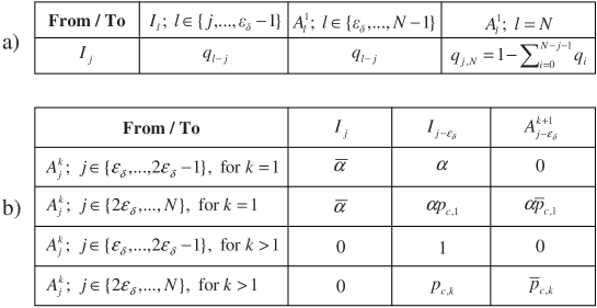
Figure 4: State transition probabilities for the DMC model in Sec. V-B: a) transition probabilities due to energy harvesting; b) transition probabilities due to the bidirectional communication with the FC. The transition matrix $\mathbf{P}$ can be derived according to the probabilities in a) and b) for all the values of $k\in\{1,...,F_{\varepsilon}\}$ and $j\in\{0,...,N\}$.

VI Backlog Estimation

In this section we propose a backlog estimation algorithm for the DFA protocol (extension to FA is straightforward). Unlike previous work on the subject [16][19], here backlog estimation is designed by accounting for the interplay of EH, capture effect and multiple access. Computational complexity of optimal estimators is generally intractable for a large number of sensors even for conventional systems (see e.g., [19]). We thus propose a low-complexity two-steps backlog estimation algorithm that, neglecting the IR index, operates in every IR as follows: i) the FC estimates the initial backlog size $B_{1}$ based on the ccdf $G_{E}\left(\varepsilon\right)$ of the ESD energy at the beginning of the current IR; ii) the backlog estimates for the next frames are updated based on the channel outcomes and the residual ESD energy.

For the first frame, the backlog size estimate and the frame length are $\hat{B}_{1}=M\alpha G_{E}\left(\varepsilon\right)$ and $L_{1}=\left\lceil\rho\hat{B}_{1}\right\rceil$, respectively. For subsequent frames, let us assume that the FC announced a frame of $L_{k}=\left\lceil\rho\hat{B}_{k}\right\rceil$ slots. The FC estimates the backlog size for frame $k+1$ by counting the number of slots that are successful ($N_{D,k}$) and collided ($N_{C,k}$) within the $k$th frame of length $L_{k}$ slots. Since the FC cannot discern exactly how many sensors transmitted in each successful slot, the estimate of the total number $C_{D,k}$ of sensors that collided in $N_{D,k}$ successful slots is $\hat{C}_{D,k}=\left(\beta_{D,k}-1\right)N_{D,k}$, with $\beta_{D,k}$ being the conditional average number of sensors that transmit in a slot given that the slot is successful (with no capture $\beta_{D,k}=1$). Similarly, for the collided slots we obtain $\hat{C}_{C,k}=\beta_{C,k}N_{C,k}$, where $\beta_{C,k}$ is now conditioned on observing a collided slot. Derivations of $\beta_{D,k}$ and $\beta_{C,k}$ are in Appendix A. Since the estimate of the total number of sensors that unsuccessfully transmitted is $\hat{C}_{k}=\hat{C}_{C,k}+\hat{C}_{D,k}$, the backlog size estimate $\hat{B}_{k+1}$ for the $(k+1)$th frame is obtained by accounting for the fraction of sensors within $\hat{C}_{k}$ that are not in energy shortage: $\hat{B}_{k+1}=\hat{C}_{k}G_{E}((k+1)\varepsilon|k\varepsilon)$, where $G_{E}((k+1)\varepsilon|k\varepsilon)=\Pr\left[E_{m}\geq(k+1)\varepsilon|E_{m}\geq k\varepsilon\right]$. The proposed backlog estimation scheme thus works as follows:

$$\hat{B}_{k}=\left\{\begin{array}[]{lc}M\alpha G_{E}\left(\varepsilon\right)&\text{if }k=1\\ \hat{C}_{k-1}G_{E}(k\varepsilon|\left(k-1\right)\varepsilon)&\text{if }k>1\end{array}\right..$$ (21)

Algorithm (21) can be applied to any $n$th IR by deriving the ESD distribution $p_{E(n)}(\cdot)$ (or $G_{E(n)}(\cdot)$) from any initial distribution $p_{E(1)}(\cdot)$, by exploiting the DMC model in Sec. V-B.

VII Numerical Results

In this section, we present extensive numerical results to get insight into the MAC protocols design. Moreover, to validate the analysis proposed in Sec. IV and Sec. V, we compare the analytical results therein with a simulated system that does not rely on simplifying assumptions $\mathcal{A}.1$ and $\mathcal{A}.2$. The performances of the backlog estimation algorithm proposed in Sec. VI are also assessed through a comparison with the ideal case of perfectly known backlog at the FC.

VII-A MAC Performance Metrics Trade-offs

The energy $E_{H,m}(n)$ harvested between two successive IRs is assumed as geometrically-distributed with $q_{i}=\Pr[E_{H,m}(n)=i\delta]=\xi(1-\xi)^{i}$, where $\xi=\delta/(\delta+\mu_{H})$. The average harvested energy normalized by $\varepsilon$, referred to as harvesting rate, is $E[E_{H,m}(n)/\varepsilon]=\mu_{H}$.

The asymptotic time efficiencies (5) for TDMA, FA and DFA protocols, are shown in Fig. 5 versus design parameter $\rho$ (recall (6)). System performance is evaluated by considering: $\mu_{H}\in\{0.15,0.35\}$, $M=400$, $\gamma_{th}=3dB$, $\alpha=0.3$; $\varepsilon$ is normalized to unity, energy unit is $\delta=1/50$ so that $\varepsilon_{\delta}=50$ and $F_{\varepsilon}=10$. We compare the analytical performance metrics derived in Sec. IV with simulated scenarios for both known and estimated backlog. While the performance of TDMA is clearly independent of $\rho$, in FA and DFA there is a time efficiency-maximizing $\rho$, which is close to one (in [8] the optimal value was $\rho=1$ since the capture effect was not considered). The effect of decreasing (or increasing) the harvesting rate $\mu_{H}$ on the TDMA time efficiency is due to the larger (or smaller) number of sensors that are in energy shortage and whose slots are not used, while it is negligible for FA and DFA due to their ability to dynamically adjust the frame size according to backlog estimates $\hat{B}_{k}$. The tight match between analytical and simulated results also validates assumptions $\mathcal{A}.1$ and $\mathcal{A}.2$ and the efficacy of the backlog estimation algorithm.

The asymptotic delivery probability, for harvesting rate $\mu_{H}$ $\in\{0.05,0.15,0.35\}$, versus design parameter $\rho$ is shown in Fig. 6 with the same system parameters as for Fig. 5. Unlike for the time efficiency, TDMA always outperforms FA and DFA in terms of delivery probability. In fact, sensors operating with TDMA and FA have the same energy consumption since they transmit at most once per IR, while possibly more than once in DFA. However, TDMA does not suffer collisions and thus it is able to eventually deliver more packets to the FC. The delivery probability strongly depends on the harvesting rate $\mu_{H}$, which influences the ESD energy distribution and consequently the energy shortage probability. Moreover, DFA outperforms FA thanks to the retransmission capability when the harvesting rate is relatively high (e.g., $\mu_{H}$$=0.35$), while for low harvesting rate (e.g., $\mu_{H}$$\in\{0.05,0.15\}$) DFA and FA perform similarly. In fact, for low harvesting rates, most of the sensors are either in energy shortage or have very low energy in their ESDs. Hence, most of the sensors that are not in energy shortage are likely to have only one chance to transmit, and thus retransmission opportunities provided by DFA are not leveraged.

The trade-off between asymptotic delivery probability (3) and asymptotic time efficiency (5) is shown in Fig. 7 for different values of the harvesting rate $\mu_{H}\in\{0.05,0.15,0.35\}$. System parameters are the same as for Fig. 5. For TDMA, the trade-off consists of a single point on the plane, whereas FA and DFA allow for more flexibility via the selection of parameter $\rho$. When increasing $\rho$ more sensors might eventually report their measures to the FC, thus increasing the delivery probability to the cost of lowering time efficiency (see Fig. 5 and 6). For FA and DFA, the trade-off curves are obtained as $\max_{\rho}\left\{p_{d}^{AS}\right\}$, s.t. $p_{t}^{AS}=\lambda$ for each achievable $\lambda$.

The impact of the capture effect on the performance metrics trade-offs is shown in Fig. 8, where we vary the SIR threshold $\gamma_{th}\in\{0.01,3,10\}dB$ and keep the harvesting rate $\mu_{H}=0.15$ fixed (other parameters are as in Fig. 5). As expected, the lower the SIR threshold $\gamma_{th}$ the higher the probability that the SIR of any of the colliding sensors is above $\gamma_{th}$, and thus the higher the performance obtained with ALOHA-based protocols. TDMA is insensitive to $\gamma_{th}$.

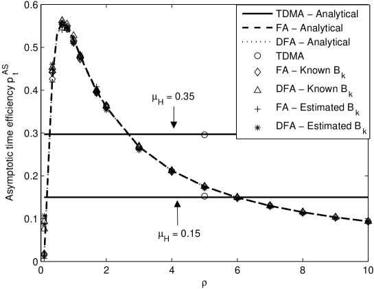
Figure 5: Asymptotic time efficiency (5) versus $\rho$, for different energy harvesting rates $\mu_{H}\in\{0.15,0.35\}$. Comparisons are between analytical derivations and simulated results with both known ($B_{k}$) and estimated backlog ($\hat{B}_{k}$, see (21)), ($M=400$, $\gamma_{th}=3dB$, $\alpha=0.3$, $F_{\varepsilon}=10$, $\varepsilon=1$, $\delta=1/50$).

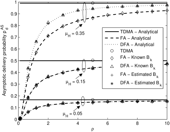
Figure 6: Asymptotic delivery probability (3) versus $\rho$, for different energy harvesting rate $\mu_{H}\in\{0.05,0.15,0.35\}$. Comparisons are between analytical derivations and simulated results with both known ($B_{k}$) and estimated backlog ($\hat{B}_{k}$, see (21)), ($M=400$, $\gamma_{th}=3dB$, $\alpha=0.3$, $F_{\varepsilon}=10$, $\varepsilon=1$, $\delta=1/50$).

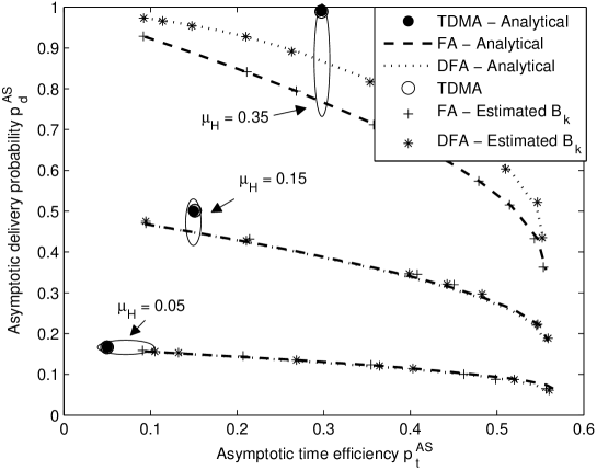
Figure 7: Trade-off between asymptotic delivery probability (3) and asymptotic time efficiency (5) for different energy harvesting rate $\mu_{H}\in\{0.05,0.15,0.35\}$. Comparisons are between analytical derivations and simulated results with estimated backlog ($\hat{B}_{k}$, see (21)), ($M=400$, $\gamma_{th}=3dB$, $\alpha=0.3$, $F_{\varepsilon}=10$, $\varepsilon=1$, $\delta=1/50$).

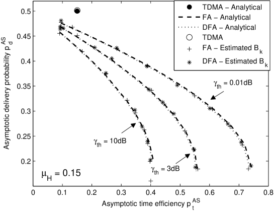
Figure 8: Trade-off between asymptotic delivery probability (3) and asymptotic time efficiency (5) for different SIR threshold $\gamma_{th}\in\{0.01,3,10\}dB$ values and fixed energy harvesting rate $\mu_{H}=0.15$. Comparisons are between analytical derivations and simulated results with estimated backlog ($\hat{B}_{k}$, see (21)), ($M=400$, $\alpha=0.3$, $F_{\varepsilon}=10$, $\varepsilon=1$, $\delta=1/50$).

VIII Conclusions

The design of medium access control (MAC) protocols for single-hop wireless sensor networks (WSNs) with energy-harvesting (EH) devices offers new challenges as compared to the standard scenario with battery-powered (BP) nodes. New performance criteria are called for, along with new design solutions. This paper addresses these issues by investigating the novel trade-off between the delivery probability, which measures the capability of a MAC protocol to deliver the measure of any sensor in the network to the intended destination (i.e., fusion center, FC) and the time efficiency, which measures the data collection rate at the FC. The analysis is focused on standard MAC protocols, such as TDMA, Framed-ALOHA (FA) and Dynamic-FA (DFA). Novel design issues are also discussed, such as backlog estimation and frame length selection. Extensive numerical results and discussions validate the proposed analytical framework and provide insight into the design of EH-WSNs.

Appendix A Average Number of Sensor Transmissions per Time-slot

The conditional averages $\beta_{D,k}$ and $\beta_{C,k}$ are calculated similarly to [8] by accounting for the capture effect and an arbitrary $\rho$. Let $Y$ be the number of simultaneous transmissions in the same slot, and let $\mathcal{U}_{k}$ and $\mathcal{C}_{k}$ respectively be the event of successful and collided slot in frame $k$, the average number of sensors per successful and collided slot are respectively

$$\beta_{D,k}=\sum_{j=1}^{\infty}j\Pr\left[Y=j|\mathcal{U}_{k}\right];\text{ }\beta_{C,k}=\sum_{j=2}^{\infty}j\Pr\left[Y=j|\mathcal{C}_{k}\right]$$ (22)

To calculate $\beta_{D,k}$ consider $\mathcal{A}.1$ and $\mathcal{A}.2$ and allow the number of possible interfering users up to infinity as in Sec. IV-A2. By exploiting the Bayes rule, we have $\Pr\left[Y=j|\mathcal{U}_{k}\right]=\Pr\left[\mathcal{U}_{k}|Y=j\right]\frac{\Pr\left[Y=j\right]}{\Pr\left[\mathcal{U}_{k}\right]}$, where $\Pr\left[\mathcal{U}_{k}|Y=j\right]=jp_{c,k}(j-1)$, $\Pr\left[Y=j\right]=e^{-\frac{1}{\rho}}/(\rho^{j}j!)$ and $\Pr\left[\mathcal{U}_{k}\right]=p_{t,k}^{DFA}$ (see 18). We can similarly obtain $\beta_{C,k}$ given that $\Pr\left[\mathcal{C}_{k}\right]=1-\Pr\left[\mathcal{U}_{k}\right]-\beta\left(0,B,L\right)$, where $\beta\left(0,B,L\right)\simeq e^{-\frac{1}{\rho}}$ is the probability of an empty slot, and $\Pr\left[\mathcal{C}_{k}|Y=j\right]=1-\Pr\left[\mathcal{U}_{k}|Y=j\right]$ for $j\geq 1$.

References

- [1] J.A. Paradiso, T. Starner, "Energy scavenging for mobile and wireless electronics," IEEE Perv. Computing Mag., vol. 4, no. 1, pp. 18-27, Jan.-Mar. 2005.
- [2] A. Kansal, J. Hsu, S. Zahedi, and M. B. Srivastava, "Power management in energy harvesting sensor networks," ACM Trans. on Embedded Computing Systems, vol. 6, no. 4, art. 32, Sep. 2007.
- [3] I.F. Akyildiz, S. Weilian, Y. Sankarasubramaniam, E. Cayirci, "A survey on sensor networks," IEEE Commun. Mag., vol. 40, no. 8, pp. 102-114, Aug. 2002.
- [4] V. Sharma, U. Mukherji, V. Joseph and S. Gupta, "Optimal energy management policies for energy harvesting sensor nodes," IEEE Trans. Wireless Commun., vol. 9, no. 4, pp. 1326-1336, Apr. 2010.
- [5] L. Ren-Shiou, P. Sinha., C.E. Koksal, "Joint energy management and resource allocation in rechargeable sensor networks," in Proc. IEEE INFOCOM, San Diego, CA, pp. 1-9, Mar. 2010.
- [6] V. Sharma, U. Mukherji, V. Joseph, "Efficient energy management policies for networks with energy harvesting sensor nodes," in Proc. Allerton Conf. Commun., Control and Computing, Monticello, IL, pp. 375-383, Sep. 2008.
- [7] D. Bertsekas, R. G. Gallager, Data networks. Prentice Hall, 1992.
- [8] F. C. Schoute, "Dynamic frame length ALOHA," IEEE Trans. Commun., vol. 31, no. 4, pp. 565-568, Apr. 1983.
- [9] C. Moser, J. Chen, L. Thiele, "An energy management framework for energy harvesting embedded systems," ACM J. on Emerging Tech. Computing Systems, vol. 6, no. 2, art. 7, Jun. 2008.
- [10] F. Iannello, O.Simeone and U. Spagnolini, "Dynamic framed-ALOHA for energy-constrained wireless sensor networks with energy harvesting," in Proc. IEEE GLOBECOM, Miami, FL, Dec. 2010.
- [11] EnOcean White Paper. [Online]. Available: http://www.enocean.com.
- [12] A. P. Sample, D. J. Yeager, P. S. Powledge, J. R. Smith, "Design of a passively-powered, programmable sensing platform for UHF RFID systems," in Proc. IEEE Int. Conf. RFID, Grapevine, TX, pp. 149-156, Mar. 2007.
- [13] EPC UHF Class 1 Gen 2. [Online]. Available: http://www.epcglobalinc.org
- [14] J. E. Wieselthier, A. Ephremides, and L. A. Michaels, "An exact analysis and performance evaluation of framed ALOHA with capture," IEEE Trans. Commun., vol. 37, no. 2, pp. 125-137, Feb. 1989.
- [15] M. Gatzianas, L. Georgiadis, L. Tassiulas, "Control of wireless networks with rechargeable batteries," IEEE Trans. Wireless Commun., vol.9, no.2, pp.581-593, Feb. 2010.
- [16] M. Kodialam and T. Nandagopal, "Fast and reliable estimation schemes in RFID systems," in Proc. MOBICOM, Los Angeles, CA, pp. 322-333, Sep. 2006.
- [17] S. Kandukuri, S. Boyd, "Optimal power control in interference-limited fading wireless channels with outage-probability specifications," IEEE Trans. Commun., vol. 1, no. 1, pp. 46-55, Jan 2002.
- [18] R. Gallager, Discrete stochastic processes. Kluwer, 1995.
- [19] B. Knerr, M. Holzer, C. Angerer, M. Rupp, "Slot-by-slot maximum likelihood estimation of tag populations in framed slotted aloha protocols," in Proc. SPECTS, Edinburgh, UK, pp. 303-308, Jun. 2008.