Information filtering via biased heat conduction

Abstract

Heat conduction process has recently found its application in personalized recommendation [T. Zhou et al., PNAS 107, 4511 (2010)], which is of high diversity but low accuracy. By decreasing the temperatures of small-degree objects, we present an improved algorithm, called biased heat conduction (BHC), which could simultaneously enhance the accuracy and diversity. Extensive experimental analyses demonstrate that the accuracy on MovieLens, Netflix and Delicious datasets could be improved by 43.5%, 55.4% and 19.2% compared with the standard heat conduction algorithm, and the diversity is also increased or approximately unchanged. Further statistical analyses suggest that the present algorithm could simultaneously identify users’ mainstream and special tastes, resulting in better performance than the standard heat conduction algorithm. This work provides a creditable way for highly efficient information filtering.

With the advent of the Internet Broder2000 and wide application of Web 2.0 techniques, there sprout many web sites that enable large communities to aggregate and interact. For example, Twitter allows its $1.7\times 10^{8}$ members to share interests and life experiences, Facebook has already exceeded 500 million members since July 16th, 2010, and their members are growing ever faster. This brings massive amount of accessible information, more than every individual’s ability to process. Searching, filtering and recommending thus become indispensable in the Internet era, in which the personalized recommender systems have become an effective tool to address the information overload problem by predicting users’ interests and habits based on their historical records. Personalized recommender systems have been used to recommend books and CDs at Amazon.com, movies at Netflix.com, and news at Versifi Technologies (formerly AdaptiveInfo.com) Adomavicius2005 . Motivated by the practical significance to e-commerce, recommender systems have caught increasing attention and become an essential issue Ecommerce2001 ; PNAS . A personalized recommender system includes three parts: data collection, model analysis and recommender algorithm, where the algorithm is the core part. Thus far, various kinds of algorithms have been proposed, including collaborative filtering (CF) approaches Herlocker2004 ; Konstan1997 ; Liu2009 ; Liu2008b ; Dun2009 ; Liu2009int , content-based analyses Balab97 ; Pazzani99 , tag-aware algorithms Zhang1 ; Zhang2 ; Zhang3 , link prediction approaches Lv1 ; Lv2 ; Lv3 , hybrid algorithms Pazzani1997 ; Good1999 , and so on. For a review of current progress, see Refs. Adomavicius2005 ; Liu2009b and the references therein.

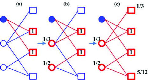
Figure 1: (Color online) Illustration of heat conduction algorithm on a bipartite user-object network: (a) The objects collected by the target user are activated, with temperature 1, while others are of temperature 0. (b) Each user’s temperature is the average over all her/his collected objects. (c) Same process happens from users to objects.

A recommender system could be described by a bipartite network ShangEPL ; LGZ2011 , in which there are two kinds of nodes: users $U$ and objects $O$. The users’ historical records are represented by the edges connecting users and objects. Supposing there are $m$ objects $O=\{o_{1},o_{2},\cdots,o_{m}\}$ and $n$ users $U$ = $\{u_{1},u_{2},$ $\cdots,$ $u_{n}\}$, the system can be fully described by an adjacency matrix ${\bf A}=\{a_{l\alpha}\}_{m,n}$, where $a_{l\alpha}=1$ if $o_{\alpha}$ is collected by $u_{l}$, and $a_{l\alpha}=0$ otherwise. A reasonable assumption is that objects collected by users are what these users like and a recommendation algorithm aims at predicting users’ personal opinions on the objects they have not yet collected Zhou2007 ; Zhang2007b ; Zhang2007a . In the standard heat conduction (HC) algorithm, we first construct a propagator matrix ${\bf W}^{h}$, where the element $w_{\alpha\beta}$ denotes the conduction rate from object $o_{\beta}$ to $o_{\alpha}$. Denote ${\bf H}$ as the temperature vector of $m$ components: the source components are of temperature 1, while the remaining components are of temperature 0. Then the temperatures associated with the remaining nodes could be calculated by solving the thermal equilibrium equation ${\bf W}^{h}{\bf H}={\bf f}$ Zhang2007a , where ${\bf f}$ is the flux vector. This is the discrete analog of $-\kappa\nabla^{2}T(\vec{r})=\vec{\nabla}\cdot\vec{J}(\vec{r})$, where $\kappa$ is the thermal conductivity, $\nabla^{2}T(\vec{r})$ is the temperature gradient and $\vec{\nabla}\cdot\vec{J}(\vec{r})$ is the local heat flux. In this paper, ${\bf H}(i)$ plays the role of $-\kappa T(\vec{r})$ and ${\bf f}(i)$ plays the role of $\vec{\nabla}\cdot\vec{J}(\vec{r})$ Zhang2007a . In the standard HC algorithm, the temperature of the collected objects is constant, and the heat will diffuse from objects to users, and then from users to objects. The temperatures of the uncollected objects are then considered as recommendation scores: the objects given higher temperatures would be recommended preferentially (see Fig.1 for an illustration). Since HC algorithm Zhang2007a is implemented based on matrix operations, it is very time-consuming and cannot be applied to large-scale systems. Zhou et al.PNAS proposed a local HC algorithm, which spreads the heat on the user-object bipartite network and can quickly generate highly diverse yet less accurate recommendations. As a benchmark for comparison, we call it standard HC algorithm (hereinafter, HC only stands for local heat conduction algorithm PNAS ).

In this Brief Report, we present the biased heat conduction (BHC) algorithm to see how objects’ degrees affect the algorithmic performance. Using data from three real systems (MovieLens, Netflix and Delicious), we show that giving higher temperatures to the large-degree objects than the standard HC algorithm could generate highly accurate and diverse recommendations.

To test the performance of a recommendation algorithm, we randomly divide a given data set into two parts: the training set and the probe set. The information contained in the probe set is not allowed to be used for recommendation, namely we provide a recommendation list for each user only based on the training set. In this Brief Report, we always keep 90% of links in the training set and 10% of links in the probe set, and employ three different metrics to measure accuracy, novelty and diversity of recommendations.

Accuracy Zhou2007 . A good recommender algorithm should rank preferable objects that match the user tastes in higher positions, i.e., the objects in the probe set (indeed being collected by users) should be put in high positions of the recommendation list. For a user $u_{i}$, if the entry $u_{i}$-$o_{j}$ is in the probe set, we measure the position of $o_{j}$ in the ordered list for $u_{i}$. For example, if there are $100$ uncollected objects for $u_{i}$ and $o_{j}$ is the 3rd one from the top, we say the position of $o_{j}$ is $3/100$, denoted by $r_{ij}=0.03$. A good algorithm is expected to give small $r_{ij}$. Therefore, the mean value of the position $\langle r\rangle$ over all entries in the probe set can be used to evaluate the algorithmic accuracy: the smaller the average ranking score Zhou2007 , the higher the algorithmic accuracy.

Novelty and diversity Zhou2007b . Since there are countless channels to obtain popular objects’ information, uncovering very specific preference, corresponding to unpopular ones, is much more significant than simply picking out what a user likes from the list of the best sellers PNAS . To measure this factor, we go simultaneously in two directions: novelty (measured by popularity) and diversity (measured by Hamming distance). The popularity is defined as average degree of all recommended objects, $\langle k\rangle$. Since it’s hard for the users to find the unpopular objects, a good algorithm should prefer to recommend small average objects. In addition, the personalized recommendation algorithm should present different recommendation lists to different users according to their tastes and habits. The diversity is quantified by the Hamming distance $S=\langle H_{ij}\rangle$, where $H_{ij}=1-Q_{ij}(L)/L$, with $L$ is the length of recommendation list and $Q_{ij}(L)$ is the number of overlapped objects in $u_{i}$’s and $u_{j}$’s recommendation lists. The larger $S$ corresponds to higher diversity.

Table 1: Basic statistics of the tested data sets.

Data Sets	Users	Objects	Links	Sparsity
MovieLens	1,574	943	82,520	$5.56\times 10^{-2}$
Netflix	10,000	6,000	701,947	$1.17\times 10^{-2}$
Delicious	10,000	232,657	1,233,997	$5.30\times 10^{-4}$

Three benchmark datasets, named MovieLens, Netflix and Delicious (See Table 1 for basic statistics), are used to test the present algorithm. The Netflix data set is a randomly sample of huge dataset provided for the Netflix Prize Netflix , and the Delicious data set is obtained by downloading publicly available data from the social bookmarking web site Delicious.com (taking care to anonymize user identity in the process). The Delicious data is inherently unary while both MovieLens and Netflix data sets contain explicit ratings from one to five. We apply a coarse-graining method to transform them into unary forms: an object is considered to be collected by a user only if the given rating is larger than 2. The sparsity of the data sets is defined as the number of links divided by the total number of user-object pairs.

Table 2: Algorithmic performance for MovieLens, Netflix and Delicious data sets on the standard HC algorithm PNAS . The popularity $\langle k\rangle$ and diversity $S$ are obtained at $L=10$.

Data Sets	$\langle r\rangle$	$\langle k\rangle$	$S$
MovieLens	0.15156	3.085	0.88196
Netflix	0.10629	1.344	0.86296
Delicious	0.26129	1.915	0.98066

Applying the standard HC algorithm on MovieLens, Netflix and Delicious data sets, $\langle r\rangle$, $\langle k\rangle$ and $S$ are shown in Table II. One can find that although the accuracy of the standard HC algorithm is poor, it provides highly diverse recommendations. We argue that the less accuracy of the standard HC algorithm lies in the fact that it assigns overwhelming priority to the small-degree objects, leading to strong bias. Therefore, the standard HC algorithm could be improved by reinforcing the influence of the large-degree objects. In the last step of the standard HC algorithm, all of the heat an object has received is divided by its degree. Although the large-degree objects could receive lots of heat, their temperatures are very low, while small-degree objects would obtain high temperatures and thus be put in the top positions of recommendation lists. A clear advantage of the standard HC algorithm is its ability to dig out the unmainstream tastes that almost can not be found by classical methods. However, users generally like popular objects and thus an algorithm should also give chance to them. We therefore propose the BHC algorithm taking into account the object degree effect in the last diffusion step. To an target object $o_{\alpha}$, instead of dividing by its degree $k(o_{\alpha})$, the final temperature is obtained dividing by $k^{\lambda}(o_{\alpha})$. The element $w_{\alpha\beta}$ of the matrix ${\bf W}^{h}$ would be $w_{\alpha\beta}=\frac{1}{k^{\lambda}(o_{\alpha})}\sum_{l=1}^{n}\frac{a_{l\alpha}a_{l\beta}}{k(u_{l})}$. Comparing with the standard HC algorithm (i.e., $\lambda=1$), the influences of large-degree objects would be strengthened if $\lambda<1$ or depressed if $\lambda>1$.

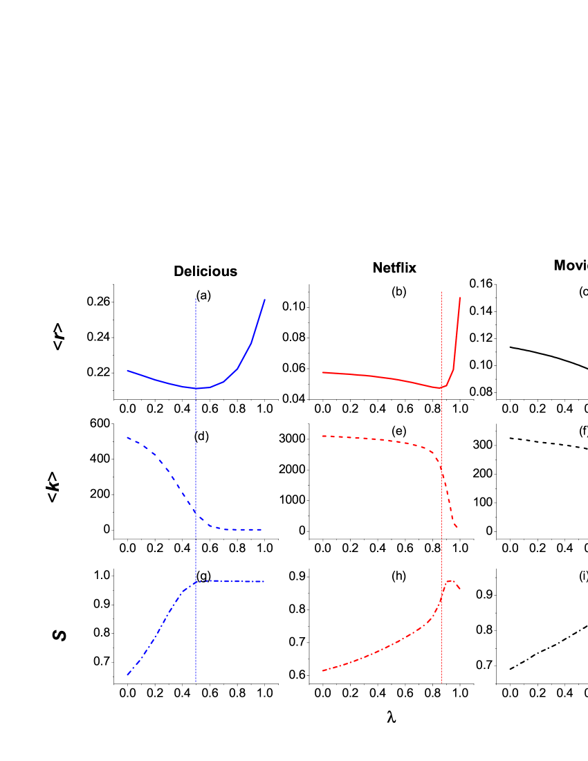
Figure 2: (Color online) Performance of the BHC algorithm on MovieLens, Netflix and Delicious data sets. The plots (a)-(c) show average ranking score $\langle r\rangle$ vs. $\lambda$. Subject to $\langle r\rangle$, the optimal $\lambda_{\rm opt}$ are 0.84, 0.85 and 0.50, and the corresponding $\langle r\rangle_{\rm opt}$ are 0.0852, 0.0474, 0.2112. The plots (d)-(f) display the results for $\langle k\rangle$ and (g)-(i) for $S$ with $L=10$. All the data points are averaged over ten independent runs with different divisions of training-probe sets.

Figure 3: The plot (a) shows the object degree distribution of Netflix data, and (b)-(d) show the correlations between the occurrence number $n(k)$ and the object degree $k$ of MD, standard HC and BHC algorithms when $L=10$. The results of MovieLens and Delicious are similar.

A summary of the primary results for BHC algorithm is given in Table III. Figure 2.(a-c) report the algorithmic accuracy $\langle r\rangle$ as a function of $\lambda$, from which one can find that the curves obtained by BHC have clear minimums. For example, the optimal parameter of MovieLens data is around $\lambda_{\rm opt}=0.84$, strongly supporting our argument that the effects of large-degree objects should be increased. Compared with the standard case (i.e. $\lambda=1$), the average ranking score $\langle r\rangle$ is reduced from 0.1516 to 0.0852 (improved by 43.5%). This results indicate that giving more opportunities to the large-degree objects will greatly increase the algorithmic accuracy. More interestingly, when $L=10$, the Hamming distance of MovieLens is also improved from 0.8820 to 0.9248 (see Fig. 2(i)), which is even better than 0.9173 obtained by the hybird algorithm PNAS . Actually, the standard HC algorithm prefers to give more opportunities to the small-degree objects and ranks them at the top positions of many users’ recommendation lists. Therefore, the Hamming distance may not be the highest although the popularity is the lowest. Figure 2(b,e,h) show the similar results on Netflix, where the optimal parameter is $\lambda_{\rm opt}=0.85$. Results of MovieLens and Netflix are very close to each other, with the fact that both data sets are movie-related and the sparsity is close. The optimal parameter $\lambda_{\rm opt}$ on Delicious (See Fig.2(a,d,g)) equals 0.5, with very small $\langle k\rangle$ and very high $S$ ($\approx 0.98$). Both the optimal ranking score $\langle r\rangle_{\rm opt}=0.2112$ and the Hamming distance $S=0.9795$ of Delicious are much larger than the ones of MovieLens and Netflix. The results are twofold: the higher sparsity of edges and the larger number of objects. The former leads to less accurate recommendation while the latter results in higher diversity.

Table 3: Algorithmic performance on BHC algorithm. The Hamming distance is corresponding to $L=10$.

Data Sets	$\lambda_{\rm opt}$	$\langle r_{\rm opt}\rangle$	Improvement	$S_{\rm opt}$
MovieLens	0.84	0.0852	43.5%	0.9248
Netflix	0.85	0.0474	55.4%	0.8200
Delicious	0.50	0.2112	19.2%	0.9795

Table IV reports the performances obtained by several algorithms on MovieLens dataset, from which one can find the accuracy $\langle r\rangle$ of BHC algorithm is close to the result of HO-CF algorithm which needs to compute the second-order similarity information, and the diversity of BHC algorithm is the highest one. In order to explain the reasons why both accuracy and diversity can be enhanced by BHC algorithm, the frequencies of appearances $n(k)$ of objects of degree $k$ in all users’ recommendation lists are investigated. We show the results of a typical example, Netflix, where the length of recommendation list is $L=10$. Different from the power-law degree distribution in Fig.3(a), $n(k)$ of BHC algorithm has butterfly shape, which means that the objects with large or small degrees are recommended more frequently. Figure 3(b) shows that mass diffusion algorithm prefers to recommend the large-degree objects, while Fig. 3(c) shows that the standard HC algorithm gives higher recommendation scores to the small-degree objects, thus the popular objects are largely depreciated. Comparing Fig. 3(c) with Fig. 3(d), at the optimal case $\lambda_{\rm opt}=0.85$, both small-degree and large-degree objects are recommended with high frequency by the BHC algorithm. In a word, the advantage of BHC is that it could not only dig out the users’ very special tastes, but also find out the common interesting objects.

Table 4: Algorithmic performance for MovieLens data. $\langle k\rangle$ and $S$ are corresponding to $L=10$. MD is abbreviations of the algorithms proposed in Ref. Zhou2007 , Heter-NBI, HO-CF, IMCF and WHC are abbreviations of algorithms with heterogeneous initial resource distribution proposed in Ref. Zhou2007b , high-order collaborative filtering (CF) algorithm proposed in Ref. NJP2009 , improved modified CF algorithm in Ref. PhysicaA2010 and the algorithm presented in Ref. LGZ2011 .

	Algorithms	$\langle r\rangle$	$S$	$\langle k\rangle$
	MD	0.1060	0.617	233
	HC	0.1516	0.750	3.09
	Heter-NBI	0.1010	0.682	220
	HO-CF	0.0826	0.9127	237
	IMCF	0.0877	0.826	175
	WHC	0.0914	0.941	179
	BHC	0.0852	0.925	197

In this Brief Report, we propose a biased heat conduction algorithm by considering the degree effects in the last step of the local heat conduction process PNAS , which could greatly improve the accuracy of the standard HC algorithm. In the standard HC algorithm, the small-degree objects are recommended overwhelmingly because in the last step, to calculate the temperature, the received heat is divided by the object degree. This division largely depresses the chance of a large-degree object to be recommended. In contrast, the power-law object degree distribution indicates that large-degree objects are preferred by many users, therefore a good algorithm should also pay attention to the them. In addition, a personalized recommender system should provide each user recommendations according to his/her own interests and habits. Therefore the diversity of recommendation lists plays a crucial role to quantify the personalization. The numerical results show that the recommendation lists generated by the BHC algorithm are of competitively higher diversity and remarkably higher accuracy than those generated by the standard HC algorithm. The statistical results on Facebook applications also show that the objects could be divided into two categories JPPNAS . One of them is collected by almost all of users, while others are only collected by small-size group users, which indicates that the users’ tastes could be expressed by two categories: popular one and special one. Therefore, the reason why BHC could produce higher accuracy is that users’ two kinds of interests could be simultaneously identified. However, how to timely track users’ current popular and special tastes is still an open problem.

We acknowledge GroupLens Research Group for providing us MovieLens data and the Netflix Inc. for Netflix data. This work is partially supported by the European Commission FP7 Future and Emerging Technologies Open Scheme Project ICTeCollective (Contract 238597), the National Natural Science Foundation of China (Grant Nos. 10905052, and 60973069), JGL is supported by Shanghai Leading Discipline Project (No. S30501) and Shanghai Rising-Star Program (11QA1404500).

References

- (1) G.-Q. Zhang, G.-Q. Zhang, Q.-F. Yang, S.-Q. Cheng, T. Zhou, New J. Phys. 10, 123027 (2008).
- (2) G. Adomavicius, and A. Tuzhilin, IEEE Trans. Know. & Data Eng. 17, 734(2005).
- (3) J. B. Schafer, J. A. Konstan, and J. Riedl, Data Mining & Knowledge Discovery, 5, 115 (2001).
- (4) T. Zhou, Z. Kuscsik, J.-G. Liu, M. Medo, J. R. Wakeling, and Y.-C. Zhang, Proc. Natl. Acad. Sci. U.S.A. 107, 4511 (2010).
- (5) J. L. Herlocker, J. A. Konstan, K. Terveen, and J. Riedl, ACM Trans. Inform. Syst. 22, 5 (2004).
- (6) J. A. Konstan, B. N. Miller, D. Maltz, J. L. Herlocker, L. R. Gordon, and J. Riedl, Commun. ACM 40, 77 (1997).
- (7) J.-G. Liu, B.-H. Wang, and Q. Guo, Int. J. Mod. Phys. C 20, 285 (2009).
- (8) J.-G. Liu, T. Zhou, H.-A. Che, B.-H. Wang, and Y.-C. Zhang, Physica A 389, 881 (2010).
- (9) D. Sun, T. Zhou, J.-G. Liu, R. -R. Liu, C. -X. Jia, and B. -H. Wang, Phys. Rev. E 80, 017101 (2009).
- (10) J.-G. Liu, T. Zhou, B.-H. Wang, Y.-C. Zhang, and Q. Guo, Int. J. Mod. Phys. C 21, 137 (2009).
- (11) M. Balabanović and Y. Shoham, Commun. ACM 40, 66 (1997).
- (12) M. J. Pazzani, Artif. Intell. Rev. 13, 393 (1999).
- (13) M.-S. Shang, and Z.-K. Zhang, Chin. Phys. Lett. 26, 118903 (2009).
- (14) Z. -K. Zhang, T. Zhou, and Y.-C. Zhang, Physica A 389, 179 (2010).
- (15) M. -S. Shang, Z.-K. Zhang, T. Zhou, and Y.-C. Zhang, Physica A 389, 1259 (2010).
- (16) T. Zhou, L. Lü, and Y.-C. Zhang, Eur. Phys. J. B 71, 623 (2009).
- (17) L. Lü and T. Zhou, Europhys. Lett. 89, 18001 (2010).
- (18) L. Lü and T. Zhou, Physica A 390, 1150 (2011).
- (19) M. Pazzani and D. Billsus, Machine Learning 27, 313 (1997).
- (20) N. Good, J. B. Schafer, J. A. Konstan, A. l. Borchers, B. Sarwar, J. Herlocker, and J. Riedl, in Proceedings of the sixteenth national conference on Artificial Intellgence, 1999, p. 439.
- (21) J. -G Liu, M. Z. -Q. Chen, J. Chen, F. Deng, H. -T. Zhang, Z. -K. Zhang, and T. Zhou. Int. J. Inf. Syst. Sci. 5, 230 (2009).
- (22) M.-S. Shang, L. Lü, Y.-C. Zhang, and T. Zhou, Europhys. Lett. 90, 48006 (2010).
- (23) J.-G. Liu, Q. Guo, and Y.-C. Zhang, Physica A 390, 2414 (2011).
- (24) Y.-C. Zhang, M. Medo, J. Ren, T. Zhou, T. Li, and F. Yang, Europhys. Lett. 80, 68003 (2008).
- (25) T. Zhou, J. Ren, M. Medo, and Y.-C. Zhang, Phys. Rev. E 76, 046115 (2007).
- (26) Y.-C. Zhang, M. Blattner, and Y.-K. Yu, Phys. Rev. Lett. 99, 154301 (2007).
- (27) T. Zhou, L.-L. Jiang, R.-Q. Su, and Y.-C. Zhang, Europhys. Lett. 81, 58004 (2008).
- (28) T. Zhou, R.-Q. Su, R.-R. Liu, L.-L. Jiang, B.-H. Wang, and Y.-C. Zhang, New J. Phys. 11, 123008 (2009).
- (29) J.-G. Liu, T. Zhou, H.-A. Che, B.-H. Wang, and Y.-C. Zhang, Physica A 389, 881 (2010).
- (30) J. Bennett and S. Lanning, in Proceedings of the KDD Cup Workshop, New York, 2010, p. 3.
- (31) J. P. Onnela and F. Reed-Tsochas, Proc. Natl. Acad. Sci. U.S.A. 107, 18375 (2010).