MASS SHELL SMEARING EFFECTS IN TOP PAIR PRODUCTION

Abstract

The top quark pair production and decay are considered in the framework of the smeared-mass unstable particles model. The results for total and differential cross sections in vicinity of $t\bar{t}$ threshold are in good agreement with the previous ones in the literature. The strategy of calculations of the higher order corrections in the framework of the model is discussed. Suggested approach significantly simplifies calculations compared to the standard perturbative one and can serve as a convenient tool for fast and precise preliminary analysis of processes involving intermediate time-like top quark exchanges in the near-threshold region.

PACS number: 11.10.St

1 Introduction

The top pair production and decay are the key processes for precision tests of the Standard Model (SM) (see e.g. Ref. [SM] and references therein). They were intensively studied in the framework of the Quantum Chromodynamics (QCD) and Electro-Weak (EW) perturbation theory during last two decades, and various methods and schemes were proposed. The major goal of these investigations is to define the basic physical parameters of the top quark, such as its mass, width and couplings with other SM particles. In the past, the top quark physics was one of the primary research objectives at Tevatron. Nowadays, the biggest attention is paid to the process of the top quark production at the LHC (see e.g. Refs. [1,2]). However, the highest precision measurements of the top quark properties can best be reached at the future Linear Collider (LC) which supposedly operates in a clean experimental environment. The top quark physics is one of the most interesting and challenging targets for future $e^{+}e^{-}$ or $\mu^{+}\mu^{-}$ LC experiments [3,4].

The top pair production is followed by a decay chain with intermediate gauge boson states, i.e. the full process under consideration is $e^{+}e^{-}\to t^{*}\bar{t^{*}}\to b\bar{b}W^{+}W^{-}\to b\bar{b}4f$. The widths of both the top quark and the $W$-boson are large, and one necessarily needs to take into account corresponding Finite-Width Effects (FWE). In the framework of the standard perturbative approach, these effects are typically described by means of dressed propagators which are regularized by the total decay width. In order to analyze the full process of the top pair production relevant for phenomenological studies, we also have to take into account the background contribution coming from many other topologically different diagrams leading to the same six-fermion final states, which is a rather non-trivial task.

The Born-level cross-sections of the processes $e^{+}e^{-}\to b\bar{b}u\bar{d}\mu^{-}\bar{\nu}_{\mu}$ and $e^{+}e^{-}\to b\bar{b}4q$ were calculated in Refs. [5,6] and [7], respectively. Other exclusive reactions with $b\bar{b}d\bar{u}\mu^{+}\nu_{\mu},\,b\bar{b}c\bar{s}d\bar{u}$ and $b\bar{b}\mu^{+}\nu_{\mu}\tau^{-}\bar{\nu}_{\tau}$ final states were considered in Ref. [4]. In particular, it was shown that the contribution of the top-pair signal $e^{+}e^{-}\to t^{*}\bar{t}^{*}\to b\bar{b}4f$ is dominant, but the background (caused by one-resonant or non-resonant diagrams) can be quite significant too. However, it can be drastically decreased by applying certain kinematical cuts on the appropriate invariant masses.

The QCD corrections for the reaction $e^{+}e^{-}\to t\bar{t}$ in the continuum above the threshold were previously obtained in Refs. [8,9]. As well as the one-loop EW corrections were calculated in many papers (for corresponding references, see e.g. Introduction in Ref. [10]). Concerning radiative corrections (RC) to reaction $e^{+}e^{-}\to b\bar{b}4f$ with six-fermion final states, the situation is more complicated and less clear [10]. At the tree level, any of the reactions receives contributions from several hundreds of diagrams. The calculations of the full $O(\alpha)$ radiative corrections are very complicated, and different approximation schemes are typically applied. The most detailed analysis of the exclusive reactions $e^{+}e^{-}\to b\bar{b}\mu^{+}\nu_{\mu}\mu^{-}\bar{\nu}_{\mu}$ and $e^{+}e^{-}\to b\bar{b}d\bar{u}\mu^{-}\bar{\nu}_{\mu}$ was performed in Ref. [10]. In this paper, the cross-sections were calculated taking into account the leading radiative corrections, such as the initial state radiation (ISR) and factorizable EW corrections to the on-shell top-pair production, to the decay of the top quark into $bW$ and to the subsequent decays of the $W$-bosons. Usually, such calculations are carried out automatically by Monte Carlo techniques (see Ref. [10] and references therein).

In this work, we consider reactions like $e^{+}e^{-}\to t^{*}\bar{t}^{*}\to b\bar{b}4f$ with any four-fermion final states $4f$. The analysis is performed in the framework of the smeared mass unstable particles model (below, SMUP model) [11,12]. Due to exact factorization at intermediate $t,\bar{t}$ and $W^{+},W^{-}$ states, the cross-section can be represented in a simple analytical form which is convenient for analytical and numerical analysis. So far, we have applied the SMUP approach only for unstable gauge boson production and decay (see e.g. Refs. [13,14,14a]). As a continuation of our earlier studies, in this work we test the SMUP approach for the case of unstable fermions, i.e., specifically, top quarks. In our calculations, we take into account NLO radiative EW and QCD factorizable corrections which dominate close to $t\bar{t}$ threshold. Also, we illustrate the influence of the mass smearing effects and various radiative corrections (RC’s) on the differential cross-sections. The results are compared with ones calculated by using the standard perturbative methods [10], where cross-sections were represented for case of full $2\to 6$ process and, separately, for the top signal contribution alone. It was shown that in the Born approximation the results coincide with a rather high precision, and deviations of the higher-order corrected results from the standard ones are at the percentage level. So, the suggested approach can be applied in a fast preliminary analysis of various complicated processes involving intermediate top quark exchanges in the Standard Model and beyond.

Note, here we do not consider the near-threshold effects caused by the generation of the coupled $t\bar{t}$ state, which were considered in detail in many previous studies (see, for instance, Ref. [15] and references therein). We postpone this issue for a forthcoming study.

2 The model cross-section of the top-pair production and decay at the tree level

The process of top-pair production with subsequent decay $e^{+}e^{-}\to t^{*}\bar{t^{*}}\to b\bar{b}W^{+}W^{-}\to b\bar{b}4f$ is schematically represented in Fig. 1. The full process contains two steps with unstable intermediate time-like states, namely, $t,\bar{t}$ and $W^{+},W^{-}$ states. In this case, as was shown in Ref. [12], the double factorization takes place and can be described in the framework of the SMUP model [11]. Due to this factorisation, the full process can be divided into three stages: $e^{+}e^{-}\to t^{*}\bar{t}^{*}$, $t^{*}\bar{t}^{*}\to b\bar{b}W^{+}W^{-}$ and $W^{+}W^{-}\to 4f$. Here, the top-quarks and $W$-bosons are treated as unstable particles, and finite-width effects should be taken into account.

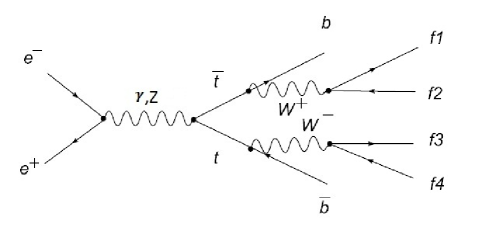
Figure 1: Feynman diagram of the top quark signal process $e^{+}e^{-}\to t^{*}\bar{t^{*}}\to b\bar{b}W^{+}W^{-}\to b\bar{b}4f$.

The SMUP model cross-section of the first reaction $e^{+}e^{-}\to t^{*}\bar{t}^{*}$ can be written as [11]

$$\sigma(e^{+}e^{-}\to t^{*}\bar{t}^{*})=\int_{m^{2}_{0}}^{s}\int_{m^{2}_{0}}^{(\sqrt{s}-m_{1})^{2}}\sigma(e^{+}e^{-}\to t(m_{1})\bar{t}(m_{2}))\rho_{t}(m_{1})\rho_{t}(m_{2})dm^{2}_{1}dm^{2}_{2},$$ (1)

where $m_{0}\approx 2M_{b}$ ($M_{b}$ is the bottom quark mass) is the threshold value of the top mass variable, $\sigma(e^{+}e^{-}\to t(m_{1})\bar{t}(m_{2}))$ is the cross-section of top pair production with random masses $m_{1}$ and $m_{2}$ and $\rho_{t}(m)$ is the probability density which describes the mass smearing of top quarks. In our calculations we take it in the Lorentzian form as [11]

$$\rho_{t}(m)=\frac{1}{\pi}\frac{m\Gamma_{t}(m)}{(m^{2}-M^{2}_{t})^{2}+m^{2}\Gamma^{2}_{t}(m)},$$ (2)

where $\Gamma_{t}(m)$ is the total decay width of the top quark with mass $m$. The decay mode $t\to bW$ has a very large branching ratio $\mathrm{Br}(t\to bW)\approx 0.999$, so formula (1) almost exactly describes the cascade process $e^{+}e^{-}\to t^{*}\bar{t}^{*}\to b\bar{b}W^{+}W^{-}$ in the stable $W$-boson approximation. In order to take into account the instability of $W$-bosons we have to express the top quark width $\Gamma_{t}(m)\approx\Gamma(t\to bW)$ in Eq. (2) as a function of smeared $W$-boson mass $\Gamma(t\to bW(M_{W}))$ with averaging over $M_{W}$. Thus, the model cross-section of the full inclusive process $e^{+}e^{-}\to t^{*}\bar{t}^{*}\to b\bar{b}W^{+}W^{-}\to b\bar{b}\sum_{f}4f$ depicted in Fig. 1 has the following convolution form:

$$\sigma(e^{+}e^{-}\to b\bar{b}\sum_{f}4f)= \int_{m^{2}_{0}}^{s}\int_{m^{2}_{0}}^{(\sqrt{s}-m_{1})^{2}}\sigma(e^{+}e^{-}\to t(m_{1})\bar{t}(m_{2}))\times$$

$$\int_{(m_{0}-M_{b})^{2}}^{(m_{1}-M_{b})^{2}}\rho_{t}(m_{1},m_{W^{+}})\rho_{W}(m_{W^{+}})dm^{2}_{W^{+}}\times$$ (3)

$$\int_{(m_{0}-M_{b})^{2}}^{(m_{2}-M_{b})^{2}}\rho_{t}(m_{2},m_{W^{-}})\rho_{W}(m_{W^{-}})dm^{2}_{W^{-}}dm^{2}_{1}dm^{2}_{2},$$

where $\rho_{W}(m)$ is defined by Eq. (2). In order to describe an exclusive reaction $e^{+}e^{-}\to t^{*}\bar{t}^{*}\to b\bar{b}f_{1}f_{2}f_{3}f_{4}$ we have to replace the total decay widths of $W$-bosons, which enter the numerator in Eq. (2), by corresponding exclusive ones (see Section 4). The same result can be obtained exactly if one calculates the cross-section of this process explicitly in the framework of the SMUP model by using dressed propagators of unstable particles (UP’s). In Ref. [12] it was shown that exact factorization of a decay chain process with UP’s in an intermediate state takes place when we exploit the model effective propagators for fermion and vector UP’s in the following form

$$\hat{D}(q)=i\frac{\hat{q}+q}{P_{F}(q)},\qquad D_{\mu\nu}(q)=-i\frac{g_{\mu\nu}-q_{\mu}q_{\nu}/q^{2}}{P_{V}(q)},$$ (4)

where $P_{F}(q)$ and $P_{V}(q)$ are the denominators of the fermion and vector boson dressed propagators, which contain corresponding total decay widths. The structure of numerators in Eq. (4) provides exact factorization and leads to a convolution-like expression (2) for the cross-section. So, there is a self-consistency between the model and UP effective theory description of the processes with UP in intermediate states. Thus, the process with a six-particles final state shown in Fig. 1 is described by a simple analytical expression (2) with four integrations over smeared unstable top and $W$-boson masses. Note, that the standard perturbative treatment of the six-particle final states in general case leads to $N=3\cdot 6-4=14$ independent parameters, from which 13 parameters have to be integrated over [16]. Such a complicated problem can be solved by using involved Monte Carlo numerical simulations only.

The results of the SMUP model calculations are presented in Fig. 2. Here, the dotted line represents the cross-section of the top-pair production in the stable particle approximation (SPA), i.e. without smearing of the top mass. The dashed line is the cross-section incorporating the top mass smearing or top finite-width effects (FWE) only, and the solid line gives the full mass smearing result, both top-quarks and $W$-bosons. Note, that the second case corresponds to the standard treatment of the process $e^{+}e^{-}\to t^{*}\bar{t}^{*}\to b\bar{b}W^{+}W^{-}$ in the stable $W$-boson approximation, and the third case – to the full process shown in Fig. 1.

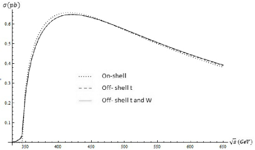
Figure 2: The cross-sections of the processes $e^{+}e^{-}\to t\bar{t}$, $e^{+}e^{-}\to b\bar{b}W^{+}W^{-}$ and $e^{+}e^{-}\to b\bar{b}\sum_{f}4f$.

From Fig. 2, one can see that the contribution of the top quarks’ FWE’s is significant (up to a few percents in the near-threshold region), while the contribution of $W$-bosons’ FWEs is small. The comparison of our results with ones in the standard perturbative treatment shows that deviations are typically very small. For instance, it was obtained in Ref. [17], that $\sigma(e^{+}e^{-}\to t^{*}\bar{t}^{*}\to b\bar{b}W^{+}W^{-})$ for $\sqrt{s}=500\,\mbox{GeV}$ is equal to 629 fb for $M_{t}=150\,\mbox{GeV}$ and 553 fb for $M_{t}=180\,\mbox{GeV}$. For the same input data, we have obtained 630 fb and 554 fb, respectively, which are in a good agreement with the result mentioned above. This comparison proves the applicability of the SMUP model fermion propagator given by the first expression in Eq. (4). In Section 4, we make such a comparison for exclusive processes as well where both SMUP model fermion and boson propagators Eq. (4) are used.

It should be noticed also that we consider the FWE’s, which are significant in the near-threshold region, but we do not include near-threshold effects caused by possible intermediate $t\bar{t}$ bound states. Since the top mean lifetime is considerably shorter than the hadronisation time, the bound state effect has no sharp resonant nature. However, it can be comparable with FWE’s or mass-smearing effects under consideration, and this problem will be considered in more detail elsewhere.

3 Factorizable corrections to the cross-section

As it was shown in previous papers [10], the EW and QCD corrections give large contributions to the cross-section of the top-pair production at energy scales close to its threshold. In this Section, we describe the strategy of our model calculations and give the total cross-section including the principal part of NLO EW and QCD corrections. Note, that the strategy of calculations and the choice of input parameters are mainly caused and defined by the effective character of the model treatment. In the framework of the SMUP model, the instability (or finite width) of unstable particles is accounted for by the smearing of their masses, i.e. by the probability density function $\rho(m)$. In turn, this function contains momentum dependent parameters $M(q)$ and $\Gamma(q)$ in analogy with the standard perturbative treatment which uses dressed propagators. So, in that sense the corrections of self-energy type are already included at the “effective” tree level, and it is reasonable to use an effective couplings, such as running coupling, absorbing the major part of vertex-type corrections.

In our calculations we have used the following input data [18]:

$$\alpha(M_{Z})=0.00781763,\,\,\,\alpha_{s}(M_{Z})=0.118,\,\,\,\sin^{2}\theta_{W}(M_{Z})=\hat{s}^{2}_{Z}=0.2313,$$

$$M_{Z}=91.1876\,\mbox{GeV},\,\,\,M_{W}=80.399\,\mbox{GeV},\,\,\,M_{t}=172.9\,\mbox{GeV}.$$ (5)

The running coupling constants $\alpha_{k}(Q^{2}),\,k=1,2,3$ were used in the one-loop approximation:

$$\alpha_{k}(Q^{2})=\frac{\alpha_{k}(M_{Z})}{1-(\beta_{k}/2\pi)\ln(Q^{2}/M^{2}_{Z})},\,\,\,\beta_{k}=(4.1,\,-19/6,\,-7).$$ (6)

The cross-sections are calculated including the following corrections:

• Vertex and self-energy type corrections for stable particles are mainly included into running couplings (6).
  

• Self-energy corrections for unstable particles are included into the probability density function $\rho(m)$, which describes the smearing of UP’s masses.
  

• Initial state radiation (ISR) is described by the photon radiation spectrum [19,20], and the bremsstrahlung from the final $t$-quark states – by vertex $Q$-dependent factor [21].
  

• QCD corrections to the top production and decay are described by the vertex multiplicative factor [21].
  

• Contribution of the box diagrams to the total cross section was evaluated at energy scales close to the threshold by using numerical FormCalc v7.3 [22] routines.

The higher order corrected cross-sections of the inclusive process $e^{+}e^{-}\to t^{*}\bar{t}^{*}\to b\bar{b}\sum_{f}4f$ are shown in Fig. 3. There, the dotted line represents the Born model cross-section, the dashed line – the cross-section with ISR and the solid line – the cross-section with total factorisable corrections (without box diagrams contribution). From the figure, one can see that the main contribution is given by ISR correction, which significantly reduces the cross-section in the near-threshold energy range and increases it at energy scales above $\sim$0.6 TeV. At large energies ($\sqrt{s}>0.5\,\mbox{TeV}$) the contribution of EW and QCD corrections becomes significant and has to be properly taken into account.

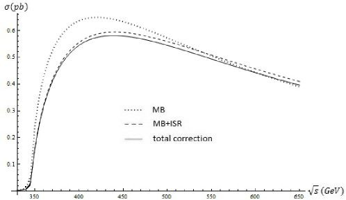
Figure 3: The higher order corrected cross-sections of the process $e^{+}e^{-}\to b\bar{b}\sum_{f}4f$.

In Fig. 4 we present the invariant mass distribution and illustrate the influence of various corrections on it. One can see that the corrections which we have taken into account according to the procedure above give noticeable contribution into this distribution in the peak area. We, also, illustrate such influence on the angular differential cross-section presented in Fig. 5. Again, we notice that this influence is quite significant and should be taken into account.

file=Massdistrib.eps,width=9cm

Figure 4: Invariant top mass distribution.

4 The cross-sections of exclusive processes

So far, we have considered the cross-section of inclusive process $e^{+}e^{-}\to t^{*}\bar{t}^{*}\to b\bar{b}\sum_{f}4f$ where the final state is summed up over all possible fermion flavors. As was noticed in the second Section, in order to get the cross-section of exclusive process $e^{+}e^{-}\to t^{*}\bar{t}^{*}\to b\bar{b}f_{1}f_{2}f_{3}f_{4}$ we can include the corresponding branching ratios $\mathrm{Br}(W\to f_{1}f_{2})$ and $\mathrm{Br}(W\to f_{3}f_{4})$. Acting this way we obtain

$$\sigma(e^{+}e^{-}\to b\bar{b}f_{1}f_{2}f_{3}f_{4})=\sigma(e^{+}e^{-}\to b\bar{b}\sum_{f}4f)\mathrm{Br}(W\to f_{1}f_{2})\mathrm{Br}(W\to f_{3}f_{4})\,.$$ (7)

where we omit intermediate virtual $t^{*}\bar{t}^{*}$ state for simplicity. This relation directly follows from the Eq. (2) when one substitutes a partial decay width of the $W$-boson into numerator of the probability distribution function $\rho_{W}(m)$ instead of the total width. It can be also derived by straightforward calculation of the $\sigma(e^{+}e^{-}\to b\bar{b}f_{1}f_{2}f_{3}f_{4})$ in the framework of the effective theory (see Ref. [12]).

file=SM_angel_diff.eps,width=8cm

Figure 5: The angular differential cross-sections for the process $e^{+}e^{-}\to b\bar{b}\sum_{f}4f$.

The expressions for the branchings ratios $\mathrm{Br}(W\to f_{1}f_{2})$ were considered in detail in Ref. [21]. Here, we use very simple but sufficiently precise formulae which incorporate QCD corrections:

$$\mathrm{Br}(W\to l\bar{\nu}_{l})=\frac{1}{9(1+2\alpha_{s}(M_{Z})/3\pi)},\,\,\,\mathrm{Br}(W\to u_{i}\bar{d}_{k})=\frac{|V_{ik}|^{2}(1+\alpha_{s}(M_{Z})/\pi)}{3(1+2\alpha_{s}(M_{Z})/3\pi)},$$ (8)

where $V_{ik}$ are elements of the Cabibbo-Kobayashi-Maskawa mixing matrix. We, also, employ the QCD corrected expression for the top quark width [21,23]:

$$\Gamma(t\to bW)=\frac{1}{16}\alpha_{2}(M_{t})|V_{tb}|^{2}\,\eta_{QCD}\,M_{t}\,f(M_{t},M_{W},M_{b}),$$ (9)

where

$$f(M_{t},M_{W},M_{b})=\lambda(M^{2}_{b},M^{2}_{W};M^{2}_{t})\left(\frac{(M^{2}_{t}-M^{2}_{b})^{2}}{M^{2}_{t}M^{2}_{W}}+\frac{M^{2}_{t}+M^{2}_{b}-2M^{2}_{W}}{M^{2}_{t}}\right);$$ (10)

$$\lambda(M^{2}_{b},M^{2}_{W};M^{2}_{t})=\left(1-2\frac{M^{2}_{b}+M^{2}_{W}}{M^{2}_{t}}+\frac{(M^{2}_{W}-M^{2}_{b})^{2}}{M^{4}_{t}}\right)^{1/2};$$

$$\eta_{QCD}=1-\frac{2\alpha_{s}(M_{t})}{3\pi}\left(\frac{2\pi^{2}}{3}-\frac{5}{2}\right).$$

Using Eqs. (7)–(9) we can calculate the exclusive cross-section for an arbitrary six-fermion final state $(b\bar{b}f_{1}f_{2}f_{3}f_{4})$. Such calculations taking into account the factorizable EW corrections were performed within the standard perturbative approach for the case of $(b\bar{b}\mu^{+}\nu_{\mu}\mu^{-}\bar{\nu}_{\mu})$ and $(b\bar{b}\mu^{+}\nu_{\mu}d\bar{u})$ final states in Ref. [10]. In this work, the full set of topologically different Born diagrams leading to the same six-fermion final state was considered. It was shown, that certain cuts on invariant masses of the $Wb$ and $f_{i}f_{k}$ pairs, which correspond to intermediate $t,\bar{t}$ and $W^{+},W^{-}$ states for signal diagrams, significantly reduce the relative contribution of the background (see Table 4).

In Tables 4 and 4 the cross-sections are given for two distinct reactions

$$(1):\quad e^{+}e^{-}\to b\bar{b}\mu^{+}\nu_{\mu}\mu^{-}\bar{\nu}_{\mu},\qquad(2):\quad e^{+}e^{-}\to b\bar{b}\mu^{+}\nu_{\mu}d\bar{u}.$$ (11)

for the energies $\sqrt{s}=430,\,500,\,1000,\,\mbox{GeV}$. In Table 4 the cross-sections are presented in the Born approximation for total set of diagrams ($\sigma_{Born}^{(k)}$(total)) and for the signal diagrams ($\sigma_{Born}^{(k)}(t^{*}\bar{t}^{*})$), where $k=1,2$ denotes the first and second reactions in Eq. (11), respectively. These values (in fb) are taken from Table 1 in Ref. [10] and are calculated with the kinematical cuts $\delta_{i}<0.1$, where $\delta_{i}$ is the deviation of the ratio $m_{i}^{inv}/M_{i}$ from unity and index $i$ is related to different $t,\bar{t},W^{+},W^{-}$ states (for more details, see Ref. [10]).

Born-level cross-sections of the processes $(1)$ and $(2)$ in Eq. (11). $\sqrt{s}$, GeV $\sigma_{Born}^{(1)}$(total) $\sigma_{Born}^{(1)}(t^{*}\bar{t}^{*})$ $\sigma_{Born}^{(2)}$(total) $\sigma_{Born}^{(2)}(t^{*}\bar{t}^{*})$ 430 5.9117 5.8642 17.727 17.592 500 5.3094 5.2849 15.950 15.855 1000 1.6387 1.6369 4.9134 4.9106

In Table 4 the results for the total cross sections (in fb) of processes $(1)$ and $(2)$ from Eq. (11) in the Born approximation are shown in the second column. The cross-sections with separate ISR and factorizable EW (FEWC) corrections are presented in the third and forth columns, respectively, and the cross-section with both the FEWC and ISR corrections included – in the fifth column. All values are calculated with the kinematical cuts mentioned above.

Comparison of the exclusive cross-sections of Ref. [11] and ones obtained in the present work. $\quad\sqrt{s},\,\rm{GeV}\quad$ $\quad\sigma^{t^{*}\bar{t}^{*}}_{\rm Born}\quad$ $\quad\sigma_{\rm Born+ISR}\quad$ $\quad\sigma_{\rm Born+FEWC}\quad$ $\quad\sigma_{\rm Born+ISR+FEWC}\quad$ $e^{+}e^{-}\to b\nu_{\mu}\mu^{+}\bar{b}\mu^{-}\bar{\nu}_{\mu}$, Ref. [10] 430 $5.8642(45)$ $5.2919(91)$ $5.6884(55)$ $5.0978(53)$ 500 $5.2849(43)$ $5.0997(51)$ $4.9909(49)$ $4.8085(48)$ 1000 $1.6369(15)$ $1.8320(18)$ $1.4243(14)$ $1.6110(16)$ $e^{+}e^{-}\to b\nu_{\mu}\mu^{+}\bar{b}\mu^{-}\bar{\nu}_{\mu}$, this work 430 $5.86476$ $5.27613$ $5.77727$ $5.19941$ 500 $5.27352$ $5.08651$ $5.18407$ $5.00291$ 1000 $1.63061$ $1.83508$ $1.58925$ $1.79079$ $e^{+}e^{-}\to b\nu_{\mu}\mu^{+}\bar{b}d\bar{u}$, Ref. [10] 430 $17.592(13)$ $15.857(20)$ $17.052(16)$ $15.283(16)$ 500 $15.855(13)$ $15.311(15)$ $14.977(16)$ $14.438(14)$ 1000 $4.9106(46)$ $5.4949(55)$ $4.2697(40)$ $4.8287(47)$ $e^{+}e^{-}\to b\nu_{\mu}\mu^{+}\bar{b}d\bar{u}$, this work 430 $17.8163$ $16.0351$ $17.5540$ $15.8019$ 500 $16.0203$ $15.4517$ $15.7516$ $15.1979$ 1000 $4.95397$ $5.57465$ $4.82889$ $5.44011$

From Table 4, it follows that the differences of the model and standard Born cross-sections are of an order of 0.1 percent and ISR correction increases it only slightly. In principle, these deviations can be further reduced. The situation becomes worse, when we take into account all major corrections. The deviations increase and become up to a few percents. This discrepancy is caused by the fact that in Ref. [10] an additional contribution from the non-signal (background) diagrams was included while we consider the signal contribution only. Moreover, we do not include the contribution of the box diagrams which becomes very important at large energies far from the threshold. According to estimations in the framework of the standard perturbative treatment, the box diagrams contribution is of an order of a few percents in the near-threshold energy range. Rough estimations in the framework of the SMUP model give the box contribution equal to $1.5-2$ percents in the energy region under consideration, and these estimations decrease the deviations. However, in the framework of the SMUP model, as well as in the effective theory of UP, the higher order corrections have an effective character, and a consistent formulation of the perturbative treatment with this model is required. This problem leads to using the model propagators inside loop diagrams, but the validity of such a procedure has still to be justified theoretically. In particular, one should first analyze the asymptotic properties of the propagators. The analysis is not carried out yet, but it is in progress now. Note, that a good agreement of the SMUP model and standard Born-level results, illustrated in Table 4, provides a good basis for such an analysis.

5 Conclusion

The production of the $t\bar{t}$ pair and its subsequent decay into six fermion final states in $e^{+}e^{-}$ annihilation has been previously analyzed within the standard perturbative treatment in a vast literature. In this work, we performed the corresponding analysis in the framework of SMUP model. So far, this approach was applied mainly to the gauge boson production, where the structure of the model boson propagators was successfully tested [13,14,14a]. In the present work, we have tested the structure of the model fermion propagator, and the top quark production mechanism has been chosen as an important example. It was shown that the results of Born-level calculations are in a good agreement with the standard perturbative ones, providing the applicability of the SMUP approach to the top-quark production and decay processes.

The SMUP model provides simple analytical expressions for the total cross-sections of inclusive and exclusive processes with top quark pair production and its subsequent decay. It is a convenient and simple instrument for description of complicated multi-step processes with unstable particles participation. The precision of this approach at the tree level is of an order of 0.1 percent or better. The method gives a possibility to include, in principle, all factorizable corrections. Our approach can be useful in a preliminary analysis of complicated processes with intermediate time-like top quark exchanges within the Standard Model and beyond.

References

- [1] D. Chakraborty, J. Konigsberg and D. L. Rainwater, Ann. Rev. Nucl. Part. Sci. 53, 301 (2003).
- [2] T. Han, Int. J. Mod. Phys. A, 23, 4107 (2008).
- [3] W. Bernreuther, J. Phys. G 35, 083001 (2008).
- [4] T. Abe et al., American Linear Collider Working Group Collaboration, SLAC-R-570, Resource book for Cnowmass 2001; arXiv:hep-ex/0106056.
- [5] K. Kolodziej, Eur. Phys. J. C 23, 471 (2002).
- [6] F. Yuasa et al.,Phys. Lett. B 414, 178 (1997).
- [7] E. Accomando et al., Nucl. Phys. B 512, 19 (1998).
- [8] F. Gangemi et al., Nucl. Phys. B 559, 3 (1999).
- [9] K. G. Chetyrkin et al., Nucl. Phys. B 482, 213 ((1996).
- [10] R. Harlander, M. Steinhauser, Eur. Phys. J. C 2, 151 (1998).
- [11] K. Kolodziej et al., Eur. Phys. J. C 46, 357 (2006).
- [12] V. I. Kuksa, Int. J. Mod. Phys. A 24, 1185 (2009).
- [13] V. I. Kuksa and N. I. Volchanskiy, Int. J. Mod. Phys. A 25, 2049 (2010).
- [14] V. I. Kuksa, R. S. Pasechnik, Int. J. Mod. Phys. A 23, 4125 (2008).
- [15] V. I. Kuksa, R. S. Pasechnik, Int. J. Mod. Phys. A 24, 5765 (2009).
- [16] R. S. Pasechnik and V. I. Kuksa, Mod. Phys. Lett. A 26, 1075 (2011).
- [17] A. H . Hoang et al., Eur. Phys. J. C 3, 1 (2000).
- [18] R. Kumar, Phys. Rev. 185, 1865 (1969).
- [19] A. Ballestrero et al., Phys. Lett. B 333, 434 (1994).
- [20] K. Nakamura et al. (Particle Data Group), J. Phys. G 37, 075021 (2010).
- [21] J. Fleisher et al., Phys. Rev. D 47, 830 (1993).
- [22] W. Beenakker et al., in Physics at LEP2, eds. G. Altarelli, T. Sjöstrand and F. Zwirner (CERN 96-01, Geneva, 1996), Vol. 1, p. 79; arXiv:hep-ph/9602351.
- [23] A. Denner, Fortschr. Phys. 41, 307 (1993).
- [24] T. Hahn and M. Perez-Victoria, Comput. Phys. Commun. 118, 153 (1999).
- [25] Guo Lei et al., Phys. Lett. B 662, 150 (2008).