Formulation and optimization of the energy-based blended quasicontinuum method

Abstract.

We formulate an energy-based atomistic-to-continuum coupling method based on blending the quasicontinuum method for the simulation of crystal defects. We utilize theoretical results from [32, 24] to derive optimal choices of approximation parameters (blending function and finite element grid) for microcrack and di-vacancy test problems and confirm our analytical predictions in numerical tests.

1. Introduction

A major goal of materials science is to predict the macroscopic properties of materials from their microscopic structure. For this purpose, it is necessary to understand the behavior of defects in these materials. We propose a computational tool, the energy-based blended quasicontinuum method (BQCE), for simulating defects such as cracks, dislocations, vacancies, and interstitials in crystalline materials.

Accurate modeling of the region near a defect requires the use of computationally expensive atomistic models. Such models are practical only for small problems. However, a defect may interact with a large region of the material through long-range elastic fields. Thus, accurate simulation of defects requires the use of a large computational domain; typically, the size required rules out the use of atomistic models for the entire region of interest.

Fortunately, the long-range elastic fields generated by a defect are well described by continuum models which can be efficiently computed using the finite-element method. Thus, defects can be accurately and efficiently simulated by coupled models which use an atomistic model near the defect and a continuum model elsewhere. We call any such model an atomistic-to-continuum coupling.

Many atomistic-to-continuum couplings have been proposed in recent years [4, 5, 21, 28, 6, 13, 16, 30]; see [19, 31] for a survey of atomistic-to-continuum couplings and computational benchmark tests. These couplings fall into two major classes: energy-based and force-based. Energy-based couplings provide an approximation to the atomistic energy of a configuration of atoms. Force-based couplings provide a non-conservative force-field which approximates the forces on each atom under the atomistic model. Our BQCE method is an energy-based coupling. Both types of couplings have intrinsic advantages; the development of energy-based couplings is especially important for finite-temperature applications since equilibrium statistical properties and transition rates can be directly approximated [10, 18].

Here, and throughout, we only consider concurrent coupling methods. An alternative approach are upscaling methods such as  [26], which achieve increased resolution near defects by adding finer scales to a coarse scale description rather than by decomposing space into fine (atomistic) and coarse (continuum) scale models.

The primary source of error for most (concurrent) energy-based couplings is the ghost force. We say that a coupling suffers from ghost forces if it predicts non-zero forces on the atoms in a perfect lattice. Although many attempts have been made to develop an energy-based coupling free from ghost forces such couplings are currently known only for a limited range of problems [30, 11, 28, 25].

Shapeev’s method [28] applies to one and two-dimensional simple crystals with an atomistic energy based on a pair interaction model, and can be extended to 3D if a modified “continuum model” is used [29]. GR-AC was proposed in [30, 11], and has recently been implemented for a two dimensional crystal with nearest neighbor many-body interactions in [25]. No ghost force free methods are currently known for three-dimensional crystals, for multi-lattice crystals (except in 1D [22]), or for atomistic models with general many-body interactions. The field-based coupling of Iyer and Gavini [16] is another interesting approach; however, it is unclear at present whether it is competitive in terms of computational complexity and generality.

In our BQCE method, the ghost forces cannot be eliminated but can be controlled in terms of an additional approximation parameter (the blending width) [24, 32]. BQCE applies to a wide range of problems for which no ghost force free methods are known; these problems include three-dimensional crystals with general many-body interactions as well as multi-lattices. This makes it an attractive method for such challenging and physically important problems.

The key feature of BQCE is a blending region where the atomistic and continuum contributions to the total energy are smoothly mixed. The ghost forces of the BQCE method can be made arbitrarily small by increasing the size of this blending region [24, 32]. BQCE shares the idea of a blending region with the bridging domain method [6], the AtC coupling [4], and the Arlequin method [5]. By contrast, the energy-based quasicontinuum method (QCE) [21], Shapeev’s method [28], and GR-AC [30, 11, 25] exhibit an abrupt transition between the atomistic and continuum models. We call any method with a blending region a blended method, and we call the weights which mix the atomistic and continuum contributions to the energy a blending function.

Both the bridging domain method and AtC coupling are very general formulations, each of them incorporating BQCE and QCE as special cases. Our BQCE formulation provides a set of specific instructions for the successful implementation of a blended method. We identify two important practical differences between BQCE and the bridging domain and AtC coupling methods. First, the BQCE method specifies a strong coupling between the atomistic and continuum regions, whereas weak couplings based on Lagrange multipliers or the penalty method have been used in most work involving the bridging domain and AtC coupling methods. Second, in BQCE, we blend the atomistic site-energy with a continuum site-energy based on the continuum site-energy defined in some formulations of the QCE method (see Section 3). This guarantees that BQCE correctly predicts the total energy of a perfect lattice subjected to uniform strain.

Our approach to blending is supported by rigorous analysis. In [32], we showed that the ghost force error of BQCE in 1D does indeed decrease with the size of the blending region, and we found that the error is minimized when the blending function is a Hermite cubic-spline. We also found that the error of the BQCE method in predicting lattice instabilities can be reduced by increasing the size of the blending region.

In this paper, we have extended the atom-based formulation (4.2) given for 1D problems in [32] to a volume-based multiD formulation (4.3) that allows finite element coarse-graining in the continuum region.

The implementation of BQCE requires the choice of two approximation parameters: a blending function $\beta$ and a finite-element mesh $\mathcal{T}$ which is used to compute the continuum contribution to the energy. In Section 4.4, we give optimal choices of $\beta$ and $\mathcal{T}$ to minimize global error norms for the problem of a point defect in a 2D crystal, based on theoretical results in [24].

We demonstrate the validity of these results in computational test problems in which we simulate a microcrack (see Figure 1) and a di-vacancy.

Outline

In Sections 2 and 3, we introduce an atomistic model for simple lattices with general many-body interactions and its corresponding continuum Cauchy–Born approximation. In Section 4, we give a precise formulation of BQCE in this setting. In Section 4.4, we offer guiding principles on choosing the blending function $\beta$ and the mesh $\mathcal{T}$ based on our analysis in [24]. The results of this analysis are summarized in Table 1. In Section 5, we describe the details of our numerical experiment. We use an atomistic energy based on the Embedded Atom Method. We did not choose our atomistic energy to model any specific physical material; instead, the atomistic energy is a toy model chosen for its simplicity. The observed rates of convergence are in agreement with the rates predicted in Section 4.4. In particular, the error of BQCE in the $W^{1,2}$ semi-norm decreases as ${\rm DoF}^{-\frac{1}{2}}$ where ${\rm DoF}$ is the number of degrees of freedom. We summarize our results and discuss open questions concerning local quantities of interest in the concluding Section 6.

2. The Atomistic Energy

Let $\Lambda$ be a $d$-dimensional Bravais lattice. We call $\Lambda$ the reference lattice. In the present work, we consider only monatomic crystals. That is, we assume that each site of the lattice $\Lambda$ is the reference position of a single atom, and that all atoms are identical. Let

$$\mathscr{Y}:=\{y:\Lambda\rightarrow\mathbb{R}^{d};y(\xi)\neq y(\eta)\mbox{ for all }\xi\neq\eta\}$$

be the set of deformations of $\Lambda$. Let $\Omega^{\rm a}\subset\Lambda$ be a finite subset of $\Lambda$. We call $\Omega^{\rm a}$ the atomistic computational domain.

In the Embedded Atom Method (EAM) [8], the energy of $\Omega^{\rm a}$ subjected to deformation $y$ takes the form

(2.1) $$\mathcal{E}^{\rm a}(y):=\sum_{\xi\in\Omega^{\rm a}}\bigg{\{}\sum_{\begin{subarray}{c}\eta\in\Lambda\\ \eta\neq\xi\end{subarray}}\frac{1}{2}\phi\big{(}|y(\eta)-y(\xi)|\big{)}+G\bigg{(}\sum_{\begin{subarray}{c}\eta\in\Lambda\\ \eta\neq\xi\end{subarray}}\rho\big{(}|y(\eta)-y(\xi)|\big{)}\bigg{)}\bigg{\}},$$

where $\phi$ is a pair potential, $\rho$ is an electron density function, and $G$ is an embedding function. We call the inner sum

(2.2) $$\mathcal{E}^{\rm a}_{\xi}(y):=\sum_{\begin{subarray}{c}\eta\in\Lambda\\ \eta\neq\xi\end{subarray}}\frac{1}{2}\phi\big{(}|y(\eta)-y(\xi)|\big{)}+G\bigg{(}\sum_{\begin{subarray}{c}\eta\in\Lambda\\ \eta\neq\xi\end{subarray}}\rho\big{(}|y(\eta)-y(\xi)|\big{)}\bigg{)}$$

the atomistic site-energy of atom $\xi$. We observe that the sum defining the energy of an atom is finite in practice even though summation ranges over the infinite lattice $\Lambda$. This is because the pair potential $\phi$ and electron density function $\rho$ are taken to have a cut-off radius $r_{c}$ such that

$$\phi(r)=\rho(r)=0\mbox{ for all }r\geq r_{c}.$$

For defining the atomistic model and the BQCE method, we can in fact consider a more general class of potentials than EAM. We only require that the total energy can be decomposed into a sum of localized site-energies associated with each atom. By localized, we mean that the energy associated with an atom $\xi$ does not depend on the positions of atoms beyond a certain cut-off distance. Such an assumption may be violated for certain energies arising from quantum mechanics, but does hold for most empirical potentials including EAM, the bond-angle potentials, and so forth. In addition, we require that the site-energies are homogeneous; that is, the energies of atoms which have the same local environment are the same.

To make these assumptions precise, we let $\mathcal{E}^{\rm a}_{\xi}(y)$ denote the site-energy associated with atom $\xi$ under deformation $y$ and require that it is of the form

(2.3) $$\mathcal{E}^{\rm a}_{\xi}(y):=V\big{(}\big{\{}y(\eta)-y(\xi):\eta\in\Lambda\setminus\{\xi\},|y(\eta)-y(\xi)|<r_{c}\big{\}}\big{)},$$

where $V$ is the site-energy potential. We assume that the resulting site-energies are twice continuously differentiable, that is, $\mathcal{E}^{\rm a}_{\xi}\in C^{2}(\mathscr{Y})$. The restricted dependence of $\mathcal{E}^{\rm a}_{\xi}$ on atoms within the cut-off radius may also be expressed in the form

$$\frac{\partial\mathcal{E}^{\rm a}_{\xi}}{\partial y(\eta)}(y)=0\mbox{ for all }\eta\mbox{ with }|y(\eta)-y(\xi)|\geq r_{c}.$$

This quantifies the requirement that the site-energy is localized.

Given $\mathcal{E}^{\rm a}_{\xi}$ we define the energy of $\Omega^{\rm a}$ subjected to a deformation $y$ by

(2.4) $$\mathcal{E}^{\rm a}(y):=\sum_{\xi\in\Omega^{\rm a}}\mathcal{E}^{\rm a}_{\xi}(y).$$

We call an energy of the form (2.4) where $\mathcal{E}^{\rm a}_{\xi}$ satisfies (2.3) homogeneous. When we define the Cauchy–Born strain energy density corresponding to (2.4) in Section 3, we use that $\mathcal{E}^{\rm a}$ is homogeneous: if $\mathcal{E}^{\rm a}$ is not homogeneous, the energy per unit volume in a perfect lattice subjected to uniform strain may be more difficult to obtain (see [1] and references therein for examples).

Remark 2.1.

The locality assumption can, in principle, be replaced by an assumption that the interaction strength decays sufficiently rapidly with increasing distance between atoms.

Remark 2.2.

Homogeneity of the site-energy is our main assumption that is violated for multi-lattices. We show in [24] how to generalize our formulation for that scenario.

3. The Cauchy–Born Site Energy

BQCE is a coupling of an atomistic energy based on (2.4) with a coarse-grained continuum elastic energy based on the Cauchy–Born strain energy density (3.1). Let $\mbox{vor}(\xi)$ denote the Voronoi cell of a site $\xi\in\Lambda$. Then the Cauchy–Born strain energy density $W:\mathbb{R}^{d\times d}\rightarrow\mathbb{R}\cup\{\pm\infty\}$ corresponding to $V$ is defined by

(3.1) $$W(F):=\frac{1}{|\mbox{vor}(0)|}\mathcal{E}^{\rm a}_{0}(y^{F}),$$

where $y^{F}\in\mathscr{Y}$ is the homogeneous deformation $y^{F}(\xi)=F\xi$. $W(F)$ may be interpreted as the energy per unit volume in $\Lambda$ subjected to strain $F$. Note that the assumption of homogeneity (2.3) ensures that $\mathcal{E}^{\rm a}_{\xi}(y^{F})=\mathcal{E}^{\rm a}_{0}(y^{F})$ for all $\xi\in\Lambda$.

We will use the Cauchy–Born strain energy density (3.1) to derive a coarse-grained continuum energy suitable for coupling with the atomistic energy (2.4). First, we define a space of coarse-grained deformations. Let $\Lambda^{\rm rep}\subset\Lambda$ denote a set of representative atoms (repatoms), let $\mathcal{T}$ be a triangulation with vertices $\Lambda^{\rm rep}$, and let $P^{1}(\mathcal{T})$ denote the set of all functions $y:\mathbb{R}^{d}\rightarrow\mathbb{R}^{d}$ that are continous and piecewise affine with respect to $\mathcal{T}$. We call $P^{1}(\mathcal{T})$ the set of coarse-grained deformations. The Cauchy–Born energy of a deformation $y\in P^{1}(\mathcal{T})$ in a domain $\Omega$ is then given by

$$\mathcal{E}^{\rm c}(y):=\int_{\Omega}W(\nabla y(x))\,dx.$$

The Cauchy–Born approximation is analyzed, for example, in [7, 12, 15].

The definition of the QCE method [21] and our construction of the BQCE method in the next section use a Cauchy–Born site-energy $\mathcal{E}^{\rm c}_{\xi}$, which is analogous to the atomistic site-energy $\mathcal{E}^{\rm a}_{\xi}$. For $y\in P^{1}(\mathcal{T})$ and $\xi\in\Lambda$, we define $\mathcal{E}^{\rm c}_{\xi}$ by

$$\mathcal{E}^{\rm c}_{\xi}(y): =\int_{\mbox{vor}(\xi)}W(\nabla y(x))\,dx$$

(3.2) $$=\sum_{T\in\mathcal{T}}|\mbox{vor}(\xi)\cap T|W(\nabla y|_{T}).$$

In formula (3.2), $|\mbox{vor}(\xi)\cap T|$ denotes the volume of the intersection of $\mbox{vor}(\xi)$ with the element $T$. We observe that the sum on the right hand side of equation (3.2) is finite because only finitely many elements $T\in\mathcal{T}$ can intersect $\mbox{vor}(\xi)$.

4. The Blended Quasicontinuum Energy

4.1. Formulation of the BQCE method

The BQCE method is an atomistic-to-continuum coupling based on the QCE method of Tadmor et al. [21]. In QCE, the reference domain $\Omega^{\rm a}$ is partitioned into an atomistic region $\mathcal{A}$ and a continuum region $\mathcal{C}$, and the QC energy $\mathcal{E}^{\rm qc}:P^{1}(\mathcal{T})\rightarrow\mathbb{R}$ is defined by

(4.1) $$\mathcal{E}^{\rm qc}(y):=\sum_{\xi\in\mathcal{A}}\mathcal{E}^{\rm a}_{\xi}(y)+\sum_{\xi\in\mathcal{C}}\mathcal{E}^{\rm c}_{\xi}(y).$$

In BQCE, the atomistic and continuum energies per atom are weighted averages. Given a blending function $\beta:\Omega^{\rm a}\rightarrow[0,1]$ the BQCE energy $\mathcal{E}^{\beta}:P^{1}(\mathcal{T})\rightarrow\mathbb{R}$ is defined by

(4.2) $$\mathcal{E}^{\beta}(y):=\sum_{\xi\in\Omega^{\rm a}}\beta(\xi)\mathcal{E}^{\rm c}_{\xi}(y)+(1-\beta(\xi))\mathcal{E}^{\rm a}_{\xi}(y).$$

We observe that the QCE energy with continuum region $\mathcal{C}$ is the same as the BQCE energy with $\beta$ chosen as the characteristic function of $\mathcal{C}$. Our formulation of BQCE is similar in spirit to the bridging domain method [6], the AtC coupling [4], and the Arlequin method [5]; it differs from [6, 4, 5] in that we specify a strong coupling between the atomistic and continuum models, and accordingly our method is based on the minimization of an energy. Moreover, our formulation in terms of atomistic and continuum energies per atom guarantees that the BQCE energy is exact under homogenous deformations.

The BQCE energy can be rewritten in the form

$$\mathcal{E}^{\beta}(y) =\sum_{\xi\in\Omega^{\rm a}}\beta(\xi)\int_{\mbox{vor}(\xi)}W(\nabla y)\,dx+(1-\beta(\xi))\mathcal{E}^{\rm a}_{\xi}(y)$$

$$=\sum_{\xi\in\Omega^{\rm a}}\sum_{T\in\mathcal{T}}\beta(\xi)|\mbox{vor}(\xi)\cap T|W(\nabla y|_{T})+\sum_{\xi\in\Omega^{\rm a}}(1-\beta(\xi))\mathcal{E}^{\rm a}_{\xi}(y)$$

(4.3) $$=\sum_{T\in\mathcal{T}}v^{\beta}_{T}W(\nabla y|_{T})+\sum_{\xi\in\Omega^{\rm a}}(1-\beta(\xi))\mathcal{E}^{\rm a}_{\xi}(y),$$

where the BQCE-effective volume of the element $T$ is defined by

(4.4) $$v^{\beta}_{T}:=\sum_{\xi\in\Omega^{\rm a}}\beta(\xi)|\mbox{vor}(\xi)\cap T|.$$

Remark 4.1.

The triangulation $\mathcal{T}$ need not cover the entire domain $\Omega^{\rm a}$. For $\mathcal{T}$ a triangulation which covers only part of $\mathbb{R}^{d}$, define

$$\Omega(\mathcal{T}): =\cup_{T\in\mathcal{T}}T,\text{ and }$$

$$P^{1}(\mathcal{T}): =\{y:\Omega(\mathcal{T})\cup\Lambda\rightarrow\mathbb{R}^{d}:\text{ y piecewise affine w.r.t. $\mathcal{T}$ on $\Omega(\mathcal{T})$}\}.$$

We observe that $\mathcal{E}^{\beta}(y)$ is defined for $y\in P^{1}(\mathcal{T})$ if for every $\xi\in\Omega^{\rm a}$ such that $\beta(\xi)>0$ we have $\emph{\mbox{vor}}(\xi)\subset\Omega(\mathcal{T})$. In particular, it is not necessary to assume that the triangulation $\mathcal{T}$ is refined to atomistic scale anywhere in the domain $\Omega^{\rm a}$. It is possible that the use of a mesh which is not refined to atomistic scale may make the implementation of BQCE easier and more efficient in some cases.

Remark 4.2 (Multi-lattices).

If one interprets a multi-lattice as a simple lattice with a basis (see, e.g., [9, 33, 24]), then the formulation of the atomistic energy (2.4) and of the BQCE energy (4.2) require no changes. The only difference is that in the general multi-lattice case, the site energy $\mathcal{E}^{\rm a}_{\xi}(y)$ has fewer symmetries (however, see[33] for examples with high symmetry).

4.2. Far-field boundary conditions

A typical application of the BQCE method is the simulation of a defect or defect region in an infinite crystal. To that end, we require far-field boundary conditions at the domain boundary. We propose two choices.

4.2.1. Dirichlet boundary conditions

Let $\mathcal{S}\subset\mathcal{T}$ be a finite subset of $\mathcal{T}$, and let $\Omega(\mathcal{S}):=\cup_{S\in\mathcal{S}}S$ be a polygonal domain. When Dirichlet boundary conditions are imposed, the deformation of the boundary $\partial\Omega(\mathcal{S})$ of $\Omega(\mathcal{S})$ is fixed to agree with some $y_{0}\in P^{1}(\mathcal{T})$. Precisely, we let

(4.5) $${\rm Adm}:=\big{\{}y\in P^{1}(\mathcal{T}):y(x)=y_{0}(x)\mbox{ for all }x\in\partial\Omega(\mathcal{S})\big{\}}$$

denote the space of admissible deformations. We then solve the problem

(4.6) $$\mbox{Find }y\in\operatorname*{argmin}_{z\in{\rm Adm}}\mathcal{E}^{\beta}(z),$$

where we interpret $\operatorname*{argmin}_{z\in{\rm Adm}}\mathcal{E}^{\beta}(z)$ as the set of local minimizers of $\mathcal{E}^{\beta}$.

4.2.2. Periodic boundary conditions

A popular method to construct artificial far-field boundary conditions is to formulate the problem in a periodic cell. To that end, suppose that $\Omega(\mathcal{T})=\mathbb{R}^{d}$, $\mathcal{T}$ is periodic, and let $\mathcal{S}\subset\mathcal{T}$ be the finite element mesh on one periodic cell. That is, suppose that for some nonsingular matrix $A\in\mathbb{R}^{d\times d}$ whose columns are elements of $\Lambda$, we have

$$\mathcal{T}=\bigcup_{n\in\mathbb{Z}^{d}}\big{\{}An+\mathcal{S}\big{\}},$$

and that the union is disjoint.

Let $F\in\mathbb{R}^{d\times d}$ be nonsingular, and call $F$ a macroscopic strain. Given $F$, we define the admissible set as

(4.7) $${\rm Adm}:=\big{\{}y\in P^{1}(\mathcal{T}):y(x+An)=y(x)+FAn\mbox{ for all }x\in\mathbb{R}^{d}\big{\}}.$$

The associated variational problem can again be stated as (4.6).

The columns of the matrix $A$ should be understood as the directions in which the displacement $u(x)=y(x)-Fx$ is periodic. Equivalently, the set $\big{\{}Ax:x\in[0,1]^{d}\big{\}}$ is a periodic cell. The macroscopic strain $F$ should be understood as the average strain imposed on the crystal. If the size of the periodic cell is large, periodic boundary conditions with macroscopic strain $F$ approximate far-field boundary conditions with uniform strain $F$ imposed at infinity.

Note that, while we only discuss a static formulation, we see no obstacle that prevents both our formulation and analysis to apply also to quasi-static problems, in which the energy is minimized at each loading step. However, we stress that further careful analysis is required to understand the accuracy, in particular stability, of the BQCE method as the deformation approaches bifurcation points (e.g., as in the formation or motion of crystal defects or the propagation of a crack).

4.3. Degrees of freedom (DoF)

In Section 4.4, we present error estimates for the BQCE method in terms of the computational complexity, by which we mean the computational cost to compute the BQCE energy and its gradient. This is proportional to the number of degrees of freedom of the space of admissible functions ${\rm Adm}$. Similarly, in Section 5, we plot errors against the number of degrees of freedom in the computed solution.

The number of degrees of freedom (DoF) is simply the size of the nonlinear system that we solve to minimize the BQCE energy. In terms of the notation introduced in the previous section, this is the number of finite element nodes in the triangulation $\mathcal{S}$ plus the number of lattice sites in $\Lambda\setminus\Omega(\mathcal{S})$ for which $\beta(\xi)<1$.

In the reduced atomistic computation, which we describe in Section 4.5.2, DoF denotes the number of unconstrained lattice sites.

4.4. Computational complexity and optimal parameters

In [24], we conjecture an error estimate for BQCE in 2D and 3D. The conjecture is based on our error analysis of BQCE in 1D [32] and on the consistency estimates for BQCE in 2D and 3D in [24]. Following [23, Sec. 7.1], we use our conjectured error estimate to derive complexity estimates, which are bounds on the error of the BQCE method in terms of the number of degrees of freedom. We use our complexity estimates to guide the choice of optimal approximation parameters $\mathcal{T}$ and $\beta$.

Let $y_{\rm a}$ be a local minimizer of the atomistic energy, and let $y_{\beta}$ be a local minimizer of BQCE with the same boundary conditions as $y_{\rm a}$. Let $h$ be the mesh size function of the triangulation $\mathcal{T}$ ($h(x)={\rm diam}(T)$ for a.e. $x\in T$), and let $\beta$ be the blending function. Then we conjecture an estimate of the form:

(4.8) $$\begin{split}{\rm Err}:=\|\nabla y_{\rm a}-\nabla y_{\beta}\|_{L^{p}}&\lesssim\|h\nabla^{2}y_{\rm a}\|_{L^{p}(C)}+\|\nabla^{2}\beta\|_{L^{p}}\\ &=:{\rm CG}+{\rm GF},\end{split}$$

for given $p\in[1,\infty]$. For $p=2$, we have proven this result in [24]; for $p\neq 2$, it would be difficult to establish this result rigorously; and for $p\in\{1,\infty\}$, it is unclear in what generality the result holds. In (4.8), $\nabla^{2}y_{\rm a}$ and $\nabla^{2}\beta$ should be interpreted as the second derivatives of smooth interpolants of $y_{\rm a}$ and $\beta$, and $C:={\rm supp}(\beta)$. The first term, ${\rm CG}=\|h\nabla^{2}y_{\rm a}\|_{L^{p}(C)}$, is the finite element coarsening error, while the second term, ${\rm GF}=\|\nabla^{2}\beta\|_{L^{p}}$, measures the effect of the ghost forces.

We now describe the problem of a point defect in a 2D crystal. To quantify the notion of a point defect, we assume that for some $\alpha>0$,

(4.9) $$|\nabla^{2}y_{\rm a}(x)|\simeq r^{-\alpha},\qquad\text{where }r=|x|.$$

It has been observed in numerical experiments that $\alpha=2$ for a dislocation, and that $\alpha=3$ for a vacancy [14, 23].

We assume that the reference domain $\Omega$ is a roughly circular region of radius $N$ atomic spacings centered at the origin. We let $K_{0}>0$ be the radius of the atomistic region surrounding the defect, and we let $K_{1}>0$ be the width of the blending region. We then choose a radial blending function $\beta$ of the form

(4.10) $$\beta(x):=\begin{cases}0&\mbox{if }r<K_{0},\\ \beta_{0}\left(\frac{|x|-K_{0}}{K_{1}}\right)&\mbox{if }K_{0}\leq r<K_{0}+K_{1},\\ 1&\mbox{if }K_{0}+K_{1}\leq r,\end{cases}$$

where $\beta_{0}:[0,1]\rightarrow[0,1]$ is a twice continuously differentiable function with $\beta_{0}(0)=\beta_{0}^{\prime}(0)=\beta_{0}^{\prime}(1)=0$ and $\beta_{0}(1)=1$.

We summarize our complexity estimates for BQCE in Table 1. These estimates are proved in [24]. We distinguish three cases based on the value of $\gamma:=\frac{\alpha p}{p+2}$. In the second column, we give the optimal rates of convergence for BQCE. The optimal rates are attained when $K_{1}$ is given in terms of $K_{0}$ by the formula appearing in the third column and when the mesh size function $h$ is given by

(4.11) $$h(x)=\left(\frac{|x|}{K_{0}}\right)^{\gamma}.$$

Remark 4.3.

When $\gamma>1$ and $\alpha>2$, another choice of parameters results in convergence at the optimal rate but with a better constant: we use

$$K_{1}=K_{0}^{\mu}\mbox{\quad for \quad}\mu=\frac{\alpha-\frac{2}{p}}{2-\frac{2}{p}}$$

in our numerical experiments below. This choice guarantees that the finite element error decreases at the same rate as the ghost force error. See [24] for additional suggestions related to choosing parameters.

Remark 4.4.

To make the explicit calculation of optimal parameters possible, we have made simplifying assumptions on the forms of $\beta$ and $h$. In (4.10), we assume that $\beta$ is radial. We explain how to construct $\beta$ given general atomistic, continuum, and blending regions in Section 5.2 below. Similarly, we assume that $h$ is continuous even though a nonconstant continuous function cannot be the mesh size function of a triangulation. In practice, we implement BQCE using a triangulation whose mesh size function approximates the continuous $h$ defined in (4.11); we explain how to do this in Section 5.2. We expect that the complexity estimates in Table 1 will hold for practical choices of $\beta$ and $h$, not only for the simplified $\beta$ and $h$ used in the derivation of the estimates.

Table 1. Complexity estimates and optimal approximation parameters for BQCE [24]. The estimates above are for the problem of a point defect in a two-dimensional crystal. The variables $K_{0}$, $K_{1}$, $N$, and $\alpha$ are defined in Section 4.4, and $\gamma:=\frac{\alpha p}{p+2}$. In all cases, the optimal rate of convergence is attained when $h=\left(\frac{|x|}{K_{0}}\right)^{\gamma}$ and when $K_{1}$ is given in terms of $K_{0}$ by the formula in the third column above.

Case	Complexity Estimate	Optimal Parameters
$\gamma>1$	$\|\nabla y_{\rm a}-\nabla y_{\beta}\|_{L^{p}}\lesssim{\rm DoF}^{\max\{\frac{1}{p}-1,\frac{1}{p}-\frac{\alpha}{2}\}}$	$K_{1}=K_{0}$
$\gamma=1$	$\|\nabla y_{\rm a}-\nabla y_{\beta}\|_{L^{p}}\lesssim{\rm DoF}^{\max\{\frac{1}{p}-1,-\frac{1}{2}\}}$	$K_{1}=K_{0}\ln\left(\frac{N}{K_{0}}\right)^{\frac{1}{2}}$
$\gamma<1$	$\|\nabla y_{\rm a}-\nabla y_{\beta}\|_{L^{p}}\lesssim{\rm DoF}^{\max\{\frac{1}{p}-1,-\frac{1}{2}\}}$	$K_{1}=K_{0}^{\gamma}N^{1-\gamma}$

Remark 4.5.

The rates of convergence depend on the geometry of the problem and on the norm in which the error is measured. We observe that the error of BQCE does not decrease with ${\rm DoF}$ when measured in the $W^{1,1}$-seminorm; see the case $p=1$ in Table 1. This is because the $W^{-1,1}$-norm of the ghost force does not decrease as the size of the blending region increases. We refer the reader to [24] for further discussion of the convergence of BQCE for other geometries and in other norms.

Remark 4.6.

We have proved that linear blending functions have a reduced rate of convergence compared to smooth blending functions of the form (4.10) (see [32] for 1D and [24] for 2D). In Table 2, we give comparative convergence rates for the problem of a point defect in a two-dimensional crystal with decay $\alpha=3.$ We emphasize, however, that this is only an asymptotic estimate. Indeed in our micro-crack experiment in Section 5.3, we observe a significant preasymptotic regime where the two blending functions yield comparable errors.

	linear BQCE	smooth BQCE
	$\|\nabla y_{\rm a}-\nabla y_{\beta}\|_{L^{p}}$	$\|\nabla y_{\rm a}-\nabla y_{\beta}\|_{L^{p}}$
$p=2$	$\lesssim{\rm DoF}^{-\frac{1}{4}}$	$\lesssim{\rm DoF}^{-\frac{1}{2}}$
$p=\infty$	$\lesssim{\rm DoF}^{-\frac{1}{2}}$	$\lesssim{\rm DoF}^{-1}$

Table 2. Complexity estimates comparing the optimized linear and smooth BQCE method for the problem of a point defect in a two-dimensional crystal with decay $\alpha=3.$

Remark 4.7.

Although our subsequent numerical experiments are restricted to defects with zero Burgers vector and consequently $\gamma>1,$ we consider more general situations in the above analysis, in order to emphasize the generality of our approach. The implementation of a/c couplings for defects with non-zero Burgers vector poses additional challenges (what should one use for the reference domain in the neighborhood of a single dislocation?) that we will address in future work. As a matter of fact, we are not aware of numerical results from a/c coupling methods, simulating a single dislocation core in an otherwise defect-free lattice (as opposed to the simulation of a dislocation pair with total zero Burgers vector).

4.5. Comparison of BQCE with other methods

We use the estimates above to compare the complexity of BQCE with direct atomistic simulation and with patch test consistent couplings, such as Shapeev’s method.

4.5.1. Shapeev’s method and other patch test consistent methods

When $\alpha$ is small (slow decay of the elastic field), BQCE converges at the same rate as patch test consistent methods such as Shapeev’s method. In fact, if $\alpha\leq 2$ (e.g., a dislocation), then the $W^{1,2}$-error of Shapeev’s method decreases as ${\rm DoF}^{-\frac{1}{2}}$ with the number of degrees of freedom [23]. We predict the same rate of convergence for BQCE when $\alpha\leq 2$. On the other hand, when $\alpha$ is larger, patch test consistent couplings may converge faster than BQCE. When $\alpha>2$ (e.g., a vacancy, microcrack, or dislocation dipole), the $W^{1,2}$-error of Shapeev’s method decreases as ${\rm DoF}^{\frac{1}{2}-\frac{\alpha}{2}}$, whereas the $W^{1,2}$-error of BQCE decreases as ${\rm DoF}^{-\frac{1}{2}}$. Roughly speaking, this is due to the fact that, for small $\alpha$, the coarse-graining error dominates, whereas for large $\alpha$, the ghost force error dominates.

According to the estimates above, Shapeev’s method always converges at least as fast as BQCE. However, we remind the reader that patch test consistent methods are currently known only for a limited range of problems [30, 11, 28, 25]. As far as we are aware, BQCE is the only convergent energy-based method for 2D or 3D crystals with general many-body interactions. Moreover, even when patch test consistent methods are known, BQCE may be an attractive method for slowly decaying defects, since it converges at the same rate as patch test consistent methods for these problems. See [24] for a more detailed analytic comparison of BQCE with Shapeev’s method.

4.5.2. Reduced atomistic computations (ATM)

In our numerical experiments below, we compare the performance of BQCE with the reduced atomistic computation (ATM), in which far-field boundary conditions are simulated by imposing Dirichlet boundary conditions directly on the atomistic model. Precisely, let $\Omega\subset\Lambda$ be an atomistic computational domain, and let $F$ be a macroscopic strain as in Section 4.2. We then define the admissible space

$${\rm Adm}:=\big{\{}y:\Lambda\rightarrow\mathbb{R}^{d}:y(\xi)=F\xi\mbox{ for all }\xi\in\Lambda\setminus\Omega\},$$

and we solve the variational problem

(4.12) $$\mbox{Find }y\in\operatorname*{argmin}_{z\in{\rm Adm}}\mathcal{E}^{\rm a}(z).$$

We regard ATM as the simplest means of simulating far-field boundary conditions, and we feel that an atomistic-to-continuum coupling is successful only when it is more accurate than ATM. In [24], we show that

$$\big{\|}\nabla y^{\Omega}_{\rm a}-\nabla y_{\rm a}\big{\|}_{L^{p}}\lesssim N^{\frac{2}{p}+1-\alpha}\simeq{\rm DoF}^{\frac{1}{p}+\frac{1}{2}-\frac{\alpha}{2}},$$

where $N$ is the diameter of $\Omega$, $y^{\Omega}_{\rm a}$ solves (4.12), ${p\in[1,\infty]}$, and $\alpha>2$. Comparing the estimate above with Table 1, we observe that BQCE converges more quickly than ATM when $\alpha<3$, at the same rate when $\alpha=3$, and more slowly when $\alpha>3,$ which we summarize in Table 3. Our numerical experiments concern the case $\alpha=3$, and we do observe that BQCE and ATM converge at the same rate. However, for optimally chosen parameters, BQCE is still much more accurate than ATM by a significant constant factor.

	BQCE	ATM	$2<\alpha$	ATM rate vs.
	$\|\nabla y_{\rm a}-\nabla y_{\beta}\|_{L^{p}}$	$\|\nabla y_{\rm a}-\nabla y_{\rm a}^{\Omega}\|_{L^{p}}$		BQCE rate
			$\alpha>3$	higher
$p=2$	$\lesssim{\rm DoF}^{-\frac{1}{2}}$	$\lesssim{\rm DoF}^{-\frac{1}{2}+\frac{1}{2}(3-\alpha)}$	$\alpha=3$	same
			$\alpha<3$	lower
			$\alpha>3$	higher
$p=\infty$	$\lesssim{\rm DoF}^{-1}$	$\lesssim{\rm DoF}^{-1+\frac{1}{2}(3-\alpha)}$	$\alpha=3$	same
			$\alpha<3$	lower

Table 3. Complexity estimates for the optimized BQCE and ATM for the problem of a point defect in a two-dimensional crystal with decay $\alpha>2$ [24]. The variable $\alpha$ is defined in Section 4.4.

5. Numerical Example

5.1. Setup of the atomistic model

In the 2D triangular lattice defined by

$$\Lambda:=\left(\begin{array}[]{cc}1&1/2\\ 0&\sqrt{3}/2\end{array}\right)\cdot\mathbb{Z}^{2}$$

we choose a hexagonal domain $\Omega^{\rm a}$ with embedded microcrack as described in Figure 1. The sidelength of the domain is $N=500$ atomic spacings, and a defect is introduced by removing a segment of atoms at the center of $\Omega^{\rm a}$, $\Lambda^{\rm def}_{11}:=\{-5e_{1},\dots,5e_{1}\}$ in the microcrack example in Section 5.3, and $\Lambda^{\rm def}_{2}:=\{0,e_{1}\}$ in the di-vacancy example in Section 5.4, where the subscripts refer to the number of atoms removed in the simulation.

We supply the domain with Dirichlet boundary conditions by setting $y_{\rm a}(\xi)=F\xi$ for $\xi\in\Lambda\setminus\Omega^{\rm a}$, where $F$ is a macroscopic strain that we will specify below.

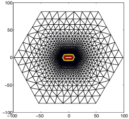
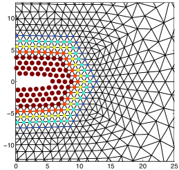
Figure 1. Deformed configuration in atomic units of a BQCE solution for a microcrack in a computational domain with approximately $3N^{2}$ atoms ($N=100$ in this figure, but $N=500$ in the benchmarks described in Sections 5.3 and 5.4). The color and size of the atom positions indicate the value of the blending function.

The site energy is given by the EAM toy-model (2.2), with

$$\phi(r)=~{} \big{[}e^{-2a(r-1)}-2e^{-a(r-1)}\big{]},\quad\rho(r)=e^{-br},\quad\text{and}$$

$$G(\bar{\rho})=~{} c\big{[}(\bar{\rho}-\bar{\rho}_{0})^{2}+(\bar{\rho}-\bar{\rho}_{0})^{4}\big{]},$$

where $a,b,c,\bar{\rho}_{0}\in\mathbb{R}$ are parameters of the model. In all our computational experiment we choose

$$a=4.4,\quad b=3,\quad c=5,\quad\bar{\rho}_{0}=6e^{-b},\quad r^{\rm cut}_{1}=1.8,\quad r^{\rm cut}_{2}=2.5.$$

The model mimics qualitative properties of practical EAM models such as those described in [17, 34].

To simplify the implementation of the model, we have introduced a cut-off in the reference configuration instead of the deformed configuration. In (2.2), we compute only sums over first, second and third neighbors. Since there are no rearrangements of atom connectivity in our experiments, we do not expect that this affects the outcome of the results.

5.2. Setup of the BQCE method

Our implementation of the BQCE method is based on (4.3), using standard finite element assembly techniques. The construction of the blending function is governed by two approximation parameters:

• $K_{0}\in\mathbb{N}$ denotes the number of atomic layers surrounding the microcrack where $\beta=1$;

• $K_{1}\in\mathbb{N}$ denotes the number of atomic layers in the blending region.

For the microcrack problem we expect $\alpha=3$ in the context of Section 4.4. Hence, according to Table 1, the choice $K_{1}:=K_{0}$ (so that the number of atoms in the atomistic region and blending region are comparable) results in the optimal rate of convergence for both $p=2$ and $p=\infty$.

Let $d_{\rm hop}(\xi,\eta)$ denote the hopping distance in the triangular lattice (with natural extension to sets), then we define

$$\Lambda^{\rm a}:=~{} \big{\{}\xi\in\Omega^{\rm a}:d_{\rm hop}(\xi,\Lambda^{\rm crack})\leq K_{0}\big{\}},\quad\text{and}$$

$$\Lambda^{\rm b}:=~{} \big{\{}\xi\in\Omega^{\rm a}:K_{0}<d_{\rm hop}(\xi,\Lambda^{\rm crack})\leq K_{0}+K_{1}\big{\}}.$$

We consider three choices of the blending function, which are all easily defined for general interface geometries:

• QCE: choosing $\beta$ to be the characteristic function of the atomistic region $\Lambda^{\rm a}$, and $K_{1}=0$, yields the QCE method defined in (4.1).

• Linear Blending: Let $d(\xi)$ denote the hopping distance from the atomistic region, then we choose

  $$\beta_{\rm lin}(\xi):=\max(1,d(\xi)/K_{1}).$$

• Smooth Blending: The three nearest-neighbour lattice vectors are given by

  $$a_{1}:=\left(\begin{array}[]{c}1\\ 0\end{array}\right),\quad a_{2}:=\left(\begin{array}[]{c}1/2\\ \sqrt{3}/2\end{array}\right),\mbox{ and }a_{3}:=\left(\begin{array}[]{c}-1/2\\ \sqrt{3}/2\end{array}\right).$$

  Define $\Delta_{i}^{2}\beta(\xi):=\beta(\xi+a_{i})-2\beta(\xi)+\beta(\xi-a_{i})$, and

  $$\Phi(\beta):=\sum_{\xi\in\Omega^{\rm a}}\sum_{i=1}^{3}|\Delta_{i}^{2}\beta(\xi)|^{2}.$$

  Then we define

  $$\qquad\quad\beta_{\rm smooth}:={\rm argmin}\big{\{}\Phi(\beta):\beta(\xi)=0\text{ in $\Lambda^{\rm a}$ and }\beta(\xi)=1\text{ in $\Omega^{\rm a}\setminus\Lambda^{\rm a}\cup\Lambda^{\rm b}$}\big{\}}.$$

  Roughly speaking, this choice generalizes the cubic spline blending suggested in [32]. It provides a practical variant for interface geometries that are not circular.

The third approximation parameter is the finite element mesh in the continuum region. We coarsen the finite element mesh away from the boundary of the blending region according to the rule suggested by the complexity estimates in Table 1. As a matter of fact it turns out that the mesh size growth is too rapid to create shape-regular meshes, hence we also impose the restriction that neighboring element can at most grow by a prescribed factor; this introduces an additional logarithmic factor in the complexity estimates [23, Sec. 7.1].

The resulting energy functional is minimized using a preconditioned Polák–Ribière conjugate gradient algorithm described in [31]. We removed the termination criterion in this algorithm and allowed it to converge to its maximal precision, that is, until the numerically computed descent direction ceases to be an actual descent direction for the energy; this occurs at an accuracy of around $10^{-5}$ in atomic units. We then perform three Newton steps, after which the residual is in the range of machine precision, to ensure that the results are not affected by the accuracy of the nonlinear solver.

5.3. Microcrack

In the microcrack experiment, we remove a long segment of atoms, $\Lambda^{\rm def}_{11}=\{-5e_{1},\dots,5e_{1}\}$ from the computational domain. The body is then loaded in mixed mode I & I​I, by setting

$$F:=\left(\begin{array}[]{cc}1&\gamma_{\rm I\!I}\\ 0&1+\gamma_{\rm I}\end{array}\right)\cdot F_{0},$$

where $F_{0}\propto I$ minimizes the Cauchy–Born stored energy function $W$, $\gamma_{\rm I}=\gamma_{\rm I\!I}=0.03$ ($3\%$ shear and $3\%$ tensile stretch).

We solve the BQCE problem (to be precise, the reduced atomistic problem (ATM) for increasing domain sizes, QCE and BQCE problems for linear and smooth blending functions) for increasing parameters $K_{0}$, and compute the error relative to the exact atomistic solution.

The relative errors in the $W^{1,2}$-seminorm are displayed in Figure 2; the relative errors in the $W^{1,\infty}$-seminorm are displayed in Figure 3; the errors in the energy are displayed in Figure 4. We observe a significant pre-asymptotic regime where the rate of convergence is faster than predicted in our theory. For larger computations, the rate of convergence approaches closely the predicted rate.

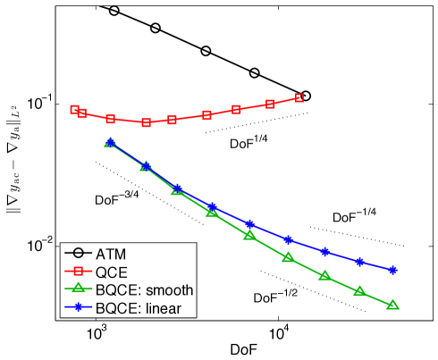
Figure 2. Convergence rates in the energy-norm (the $H^{1}$-seminorm) for the microcrack benchmark problem described in Section 5.3. This corresponds to the case $p=2$ and $\alpha=3$ in Table 1. In the above, $y_{\rm a}$ denotes the minimizer of the atomistic energy, and $y_{\rm ac}$ denotes the corresponding minimizer of the ATM, QCE or BQCE problems.

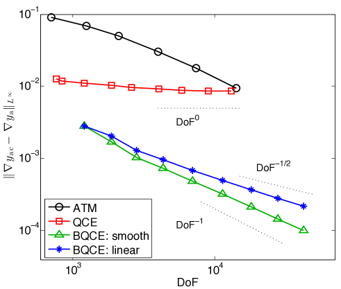
Figure 3. Convergence rates in the $W^{1,\infty}$-seminorm for the microcrack benchmark problem described in Section 5.3. This corresponds to the case $p=\infty$ and $\alpha=3$ in Table 1. In the above, $y_{\rm a}$ denotes the minimizer of the atomistic energy, and $y_{\rm ac}$ denotes the corresponding minimizer of the ATM, QCE or BQCE problems.

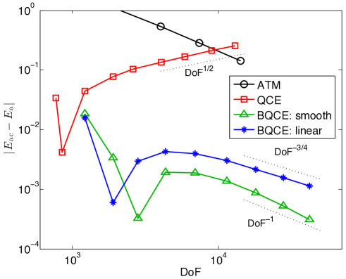
Figure 4. Convergence rates in the energy, for the microcrack benchmark problem described in Section 5.3. In the above, $E_{\rm a}$ denotes the minimum of the atomistic energy, and $E_{\rm ac}$ denotes the minimum of either the ATM, QCE or BQCE energies.

In particular, it is worth noting that the advantage of a smooth blending function only becomes significant in the asymptotic regime and is less pronounced than our theory might suggest. Since the precomputation of $\beta_{\rm smooth}$ is computationally cheap and straightforward, we nevertheless propose the choice $\beta_{\rm smooth}$ for most simulations.

Finally, we remark that the initial dip in the energy error in Figure 4 is most likely due to a change of sign in the energy error.

5.4. Di-vacancy

We perform a second numerical experiment, in order to demonstrate that the effects we observed in the microcrack example, which are not covered by our theory, are indeed caused by a pre-asymptotic regime. To this end we consider a di-vacancy defect, where only two neighboring sites $\Lambda^{\rm def}_{2}:=\{0,e_{1}\}$ are removed from the lattice. We apply 3% isotropic stretch and 3% shear loading, by setting

$$F:=\left(\begin{array}[]{cc}1+s&\gamma_{\rm I\!I}\\ 0&1+s\end{array}\right)\cdot F_{0},$$

where $F_{0}$ minimizes $W$, $s=\gamma_{\rm I\!I}=0.03$.

The relative errors in the $W^{1,2}$-seminorm are displayed in Figure 5; the relative errors in the $W^{1,\infty}$-seminorm are displayed in Figure 6; the errors in the energy are displayed in Figure 7. For the $W^{1,2}$ and $W^{1,\infty}$-seminorms we now observe precisely the rates of convergence ${\rm DoF}^{-1/2}$ and ${\rm DoF}^{-1}$ predicted by our theory. However, we observe a convergence rate ${\rm DoF}^{-3/2}$ for the energy, rather than the square of the rate for the $W^{1,2}$-seminorm which is ${\rm DoF}^{-1}$. We can, at present offer no rigorous explanation for this improved convergence rate, but speculate that it is caused by a cancellation effect that is not captured by our theory.

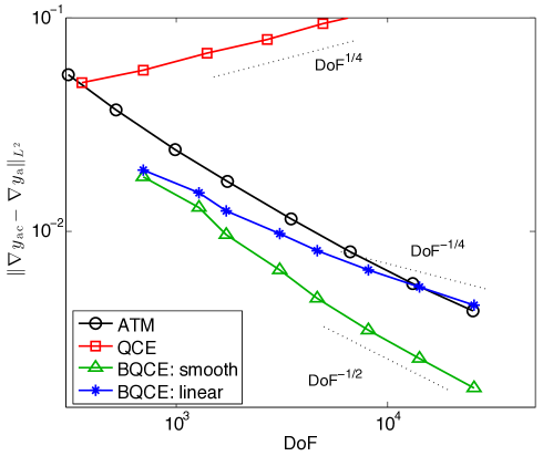
Figure 5. Convergence rates in the energy-norm (the $H^{1}$-seminorm) for the di-vacancy benchmark problem described in Section 5.4. This corresponds to the case $p=2$ and $\alpha=3$ in Table 1. In the above, $y_{\rm a}$ denotes the minimizer of the atomistic energy, and $y_{\rm ac}$ denotes the corresponding minimizer of either the ATM, BQCE or QCE problems.

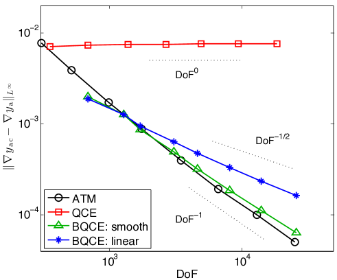
Figure 6. Convergence rates in the $W^{1,\infty}$-seminorm for the di-vacancy benchmark problem described in Section 5.4. This corresponds to the case $p=\infty$ and $\alpha=3$ in Table 1. In the above, $y_{\rm a}$ denotes the minimizer of the atomistic energy, and $y_{\rm ac}$ denotes the corresponding minimizer of the ATM, BQCE or QCE problems.

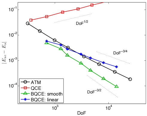
Figure 7. Convergence rates in the energy, for the di-vacancy benchmark problem described in Section 5.4. In the above, $E_{\rm a}$ denotes the minimum of the atomistic energy, and $E_{\rm ac}$ denotes the corresponding minimum of either the ATM, QCE or BQCE energies.

It is important to point out that, in this second numerical experiment, BQCE is not substantially more efficient than ATM. In fact, in the $W^{1,\infty}$-seminorm the errors are almost identical. This example clearly demonstrates that an atomistic coarse-graining scheme need not always lead to improved computational results, but that the improvement over a judiciously performed atomistic simulation is highly problem dependent. We also remark that for similar examples (e.g., a single vacancy with $F=F_{0}$), we observed that ATM has a higher accuracy than BQCE in both the $W^{1,2}$ and $W^{1,\infty}$-seminorms.

6. Conclusion

We have formulated an atomistic-to-continuum coupling, which we call the blended energy-based quasicontinuum method (BQCE). Our formulation requires only two approximation parameters for the implementation of BQCE: the blending function $\beta$ and the finite element mesh $\mathcal{T}$. For the problems of a microcrack and a di-vacancy in a two-dimensional crystal, we utilized theoretical results from [24] to obtain optimal choices of approximation parameters (blending function and finite element grid) to minimize a global error norm and confirmed our analytical predictions in numerical tests.

An interesting open question is how well different atomistic-to-continuum couplings (in particular, QCE, BQCE and the patch test consistent methods) perform if the quantity of interest is localized in the atomistic region. In [27], this question was investigated through a series of numerical experiments in which the Arlequin method was used to simulate a one-dimensional chain with a defect. The authors concluded that the local error of the Arlequin method could be controlled by moving the blending region away from the defect and increasing its size. For the quasicontinuum method, local quantities of interest were investigated in [2, 3, 20]. We hope to develop rigorous error estimates and optimal approximation parameters for localized quantities of interest in a future work.

At present BQCE is a competitive choice for numerical simulations of atomistic multi-scale problems as it applies to a much broader class than any known patch test consistent method. For example, Shapeev’s method applies only to two-dimensional, simple lattice crystals with pair interactions. Our BQCE method can be applied to challenging and physically important problems featuring three-dimensional, multi-lattice crystals and arbitrary many-body interaction potentials.

References

- [1] A. Abdulle, P. Lin, and A. V. Shapeev. Numerical methods for multilattices. arXiv:1107.3462.
- [2] Marcel Arndt and Mitchell Luskin. Error estimation and atomistic-continuum adaptivity for the quasicontinuum approximation of a Frenkel-Kontorova model. SIAM J. Multiscale Modeling & Simulation, 7:147–170, 2008.
- [3] Marcel Arndt and Mitchell Luskin. Goal-oriented adaptive mesh refinement for the quasicontinuum approximation of a Frenkel-Kontorova model. Computer Methods in Applied Mechanics and Engineering, 197:4298–4306, 2008.
- [4] S. Badia, M. Parks, P. Bochev, M. Gunzburger, and R. Lehoucq. On atomistic-to-continuum coupling by blending. Multiscale Model. Simul., 7(1):381–406, 2008.
- [5] P. T. Bauman, H. B. Dhia, N. Elkhodja, J. T. Oden, and S. Prudhomme. On the application of the Arlequin method to the coupling of particle and continuum models. Comput. Mech., 42(4):511–530, 2008.
- [6] T. Belytschko and S. P. Xiao. Coupling methods for continuum model with molecular model. International Journal for Multiscale Computational Engineering, 1:115–126, 2003.
- [7] X. Blanc, C. Le Bris, and P.-L. Lions. From molecular models to continuum mechanics. Arch. Ration. Mech. Anal., 164(4):341–381, 2002.
- [8] M. S. Daw and M. S. Baskes. Embedded-Atom Method: Derivation and Application to Impurities, Surfaces, and other Defects in Metals. Phys. Rev. B 20, 1984.
- [9] M. Dobson, R. Elliot, M. Luskin, and E. Tadmor. A multilattice quasicontinuum for phase transforming materials: Cascading cauchy born kinematics. Journal of Computer-Aided Materials Design, 14:219–237, 2007.
- [10] L. M. Dupuy, E. B. Tadmor, F. Legoll, R. E. Miller, and W. K. Kim. Finite-temperature quasicontinuum. manuscript, 2011.
- [11] W. E, J. Lu, and J. Yang. Uniform accuracy of the quasicontinuum method. Phys. Rev. B, 74(21):214115, 2006.
- [12] W. E and P. Ming. Cauchy-Born rule and the stability of crystalline solids: static problems. Arch. Ration. Mech. Anal., 183(2):241–297, 2007.
- [13] H. Fischmeister, H. Exner, M.-H. Poech, S. Kohlhoff, P. Gumbsch, S. Schmauder, L. S. Sigi, and R. Spiegler. Modelling fracture processes in metals and composite materials. Z. Metallkde., 80:839–846, 1989.
- [14] F. C. Frank and J. H. van der Merwe. One-dimensional dislocations. I. static theory. Proc. R. Soc. London, A198:205–216, 1949.
- [15] T. Hudson and C. Ortner. On the stability of bravais lattices and their cauchy–born approximations. M2AN Math. Model. Numer. Anal., 46, 2012.
- [16] M. Iyer and V. Gavini. A field theoretical approach to the quasi-continuum method. Journal of the Mechanics and Physics of Solids, 59(8):1506 – 1535, 2011.
- [17] R. A. Johnson and D. J. Oh. Analytic embedded atom method model for bcc metals. Journal of Materials Research 4, 1195–1201, 1989.
- [18] W. K. Kim, E. B. Tadmor, M. Luskin, D. Perez, and A. Voter. Hyper-qc: An accelerated finite-temperature quasicontinuum method using hyperdynamics. manuscript, 2011.
- [19] R. Miller and E. Tadmor. A unified framework and performance benchmark of fourteen multiscale atomistic/continuum coupling methods. Modelling Simul. Mater. Sci. Eng., 17, 2009.
- [20] J. T. Oden, S. Prudhomme, and P. Bauman, Error control for molecular statics problems, Int. J. Multiscale Comput. Eng., 4 (2006), pp. 647–662.
- [21] M. Ortiz, R. Phillips, and E. B. Tadmor. Quasicontinuum analysis of defects in solids. Philosophical Magazine A, 73(6):1529–1563, 1996.
- [22] C. Ortner and A. Shapeev. work in progress.
- [23] C. Ortner and A. V. Shapeev. Analysis of an Energy-based Atomistic/Continuum Coupling Approximation of a Vacancy in the 2D Triangular Lattice. ArXiv e-prints, 1104.0311, Apr. 2010.
- [24] C. Ortner and B. Van Koten. manuscript.
- [25] C. Ortner and L. Zhang. Construction and sharp consistency estimates for atomistic/continuum coupling methods with general interfaces: a 2d model problem. arXiv:1110.0168.
- [26] H. Park, E. Karpov, P. Klein, and W.K.Liu. Three-dimensional bridging scale analysis of dynamic fracture. Journal of Computational Physics, 207:588–609, 2005.
- [27] S. Prudhomme, H. Ben Dhia, P. T. Bauman, N. Elkhodja, and J. T. Oden. Computational analysis of modeling error for the coupling of particle and continuum models by the Arlequin method. Comput. Methods Appl. Mech. Engrg., 197(41-42):3399–3409, 2008.
- [28] A. Shapeev. Consistent energy-based atomistic/continuum coupling for two-body potentials in one and two dimensions. Multiscale Model. Simul., 9(3):905–932, 2011.
- [29] A. V. Shapeev. Consistent energy-based atomistic/continuum coupling for two-body potentials in three dimensions. arXiv:1108.2991.
- [30] T. Shimokawa, J. Mortensen, J. Schiotz, and K. Jacobsen. Matching conditions in the quasicontinuum method: Removal of the error introduced at the interface between the coarse-grained and fully atomistic region. Phys. Rev. B, 69(21):214104, 2004.
- [31] B. Van Koten, X. H. Li, M. Luskin, and C. Ortner. A computational and theoretical investigation of the accuracy of quasicontinuum methods. In I. Graham, T. Hou, O. Lakkis, and R. Scheichl, editors, Numerical Analysis of Multiscale Problems, volume 83 of Lect. Notes Comput. Sci. Eng. Springer, 2012. arXiv:1012.6031.
- [32] B. Van Koten and M. Luskin. Analysis of energy-based blended quasi-continuum approximations. SIAM Journal on Numerical Analysis, 49(5):2182–2209, 2011.
- [33] B. Van Koten and C. Ortner. Symmetries of 2-lattices and second order accuracy of the Cauchy–Born model. arXiv:1203.5854.
- [34] R.R. Zope and Y. Mishin. Interatomic potentials for atomistic simulations of the Ti-Al system. Phys. Rev. B 68, 024102, 2003.