Performance Analysis of Bidirectional Relay Selection with Imperfect Channel State Information

Abstract

In this paper, we investigate the performance of bidirectional relay selection using amplify-and-forward protocol with imperfect channel state information, i.e., delay effect and channel estimation error. The asymptotic expression of end-to-end SER in high SNR regime is derived in a closed form, which indicates that the delay effect causes the loss of both coding gain and diversity order, while the channel estimation error merely affects the coding gain. Finally, analytical results are verified by Monte-Carlo simulations.

I Introduction

Bidirectional relay communications, in which two sources exchange information through intermediate relays, have gained a lot of interest by now, and different transmission schemes have been proposed [1]. In [2, 3], an amplify-and-forward (AF) based network coding scheme, named as analog network coding (ANC), was introduced. With ANC, the data transmission process can be divided into two phases, and the spectral efficiency, which is restricted by half-duplex antennas, can get improved. Recently, relay selection (RS) for bidirectional relay networks has been intensively researched to achieve full spatial diversity and better system performance, which requires fewer orthogonal resources in comparison of all-participate relay approaches[4, 5]. Performing RS, the “best” relay is firstly selected before data transmission by the predefined criterion [6, 7, 8, 9, 10, 11]. In [6, 7], the authors proposed the max-min sum rate selection criterion for AF bidirectional relay. In [8, 9, 10, 11], selection criterions in minimizing the symbol error rate (SER) were introduced and analyzed.

To the authors’ best knowledge, most works about RS in bidirectional relay only consider perfect channel state information (CSI). However, imperfect CSI, i.e., delay effect and channel estimation error (CEE), has great impact on the performance of bidirectional relay selection. Specifically, the time delay between relay selection and data transmission causes that the selected relay may not be optimal for data transmission[12, 13, 14]. And similarly, channel estimation errors can not be ignored either [15, 16, 17, 18]. In [18], the authors analyzed the performance loss of bidirectional relay selection using decode-and-forward protocol with CEE, but the impact of imperfect CSI on a general bidirectional AF relay selection was not provided.

In light of the aforementioned researches, we analyze the impact of imperfect CSI, including delay effect and CEE, for bidirectional AF relay selection in this paper, which has not been studied previously. The asymptotic expression of end-to-end SER is derived in a closed form, and verified by computer simulations. Analytical and simulated results reveal that delay effect reduces both the diversity order and the coding gain, while channel estimation error merely causes the coding gain loss. The main contribution of this paper can be summarized as follows:

1. The asymptotic SER expression for bidirectional relay selection is provided in a closed form, which matches the simulated results in high SNR regime;

2. Imperfect CSI, i.e., delay and channel estimation errors, is taken into account to derive the analytical results, and its therein impact is investigated.

The remainder of this paper is organized as follows: In Section II, the system model of bidirectional AF relay selection, and the imperfect CSI model are described in detail. Section III provides the analytical expression of bidirectional relay selection with imperfect CSI. Simulation results and performance analysis are presented in Section IV. Finally, section V concludes this paper.

Notation:$\left(\cdot\right)^{*}$ and $\left|\cdot\right|$ represent the conjugate and the absolute value, respectively. $\mathbb{E}$ is used for the expectation and $Pr$ represents the probability. The probability density function and the cumulative probability function of variable $x$ are denoted by $f_{x}\left(\cdot\right)$ and $F_{x}\left(\cdot\right)$, respectively.

II System Model

The system investigated in this paper is a general bidirectional AF relay network with two sources $S_{j}$, $j=1,2$ exchanging information through the intermediate $N$ relays $R_{i}$, $i=1,\ldots,N$. The direct link between $S_{1}$ and $S_{2}$ does not exist, and each node is equipped with a single half-duplex antenna. The transmit power of the sources is assumed to be the same, denoted by $p_{s}$, and all the relays have the individual power constraint, denoted by $p_{r}$. The channel coefficients between sources and relays are reciprocal, and these coefficients are constant over the duration of one data block.

The whole procedure of bidirectional AF relay selection is divided into two parts periodically: relay selection process and data transmission process, which will be described concretely in the next section. Let $h_{s,ji}$ and $\hat{h}_{s,ji}$ represent the actual and the estimated channel coefficients between $S_{j}$ and $R_{i}$ during the relay selection process, respectively; let $h_{t,ji}$ and $\hat{h}_{t,ji}$ represent the actual and the estimated channel coefficients between $S_{j}$ and $R_{i}$ during the data transmission process, respectively. All the actual channel coefficients are independent identically distributed (i.i.d.) Rayleigh flat-fading with zero mean and unit variance, i.e., $\mathbb{E}\left(\left|{h_{t,ji}}\right|^{2}\right)=\mathbb{E}\left(\left|{h_{s,ji}}\right|^{2}\right)=1$, and thus, $\left|{h_{s,ji}}\right|^{2}$ and $\left|{h_{t,ji}}\right|^{2}$ are both exponentially distributed with unit mean. Both the sources can know the global channel coefficients by estimating the training symbols, while each relay only has its local channel information.

II-A Model of Delay Effect

Due to the time delay between relay selection process and data transmission process, $h_{s,ji}$ is not the same as $h_{t,ji}$, which means the CSI is outdated. Their relationship can be modeled by the first-order autoregressive model[14]:

$$h_{t,ji}=\rho_{f_{j}}h_{s,ji}+\sqrt{1-\rho_{f_{j}}^{2}}\varepsilon_{j}~{},$$ (1)

where $h_{t,ji}$ is a zero mean complex-Gaussian RV with variance of $\sigma_{h_{t,ji}}^{2}$; $h_{s,ji}$ and $\varepsilon_{j}$ are i.i.d. random variable (RVs) with zero mean and variance of $\sigma_{h_{s,ji}}^{2}$ and $\sigma_{\varepsilon_{j}}^{2}$, respectively. In this paper, we assume $\sigma_{h_{t,ji}}^{2}=\sigma_{h_{s,ji}}^{2}=\sigma_{\varepsilon_{j}}^{2}=1$.

The correlation coefficient $\rho_{f_{j}}$ ( $0\leq\rho_{f_{j}}\leq 1$, where $\rho_{f_{j}}=1$ represents no delay effect, in other words, the CSI is not outdated) between $S_{j}$ and relays is defined by Jakes’ autocorrelation model [14]:

$$\rho_{f_{j}}=J_{0}\left(2\pi f_{d_{j}}T\right)~{},$$ (2)

where $J_{0}\left(\cdot\right)$ stands for the zeroth order Bessel function[23], $f_{d_{j}}$ is the Doppler frequency, and $T$ is the time delay between the relay selection process and the data transmission process. In this paper, two variables $\rho_{f_{j}}$, $j=1,2$ are used to represent the correlation coefficients between $S_{j}$ and the relays, respectively, for $f_{d_{1}}$ and $f_{d_{2}}$ may be different.

II-B Model of Channel Estimation Error

Let $h$ denote the actual channel coefficient and $\hat{h}$ represent the estimated channel coefficient, and then their relationship can be modeled as follows[15]:

$$\hat{h}=h+e~{},$$ (3)

and

$$h=\rho_{e}\hat{h}+d~{}~{},$$ (4)

where $h$ and CEE $e$ are independent complex-Gaussian RVs with zero mean and variances of $\sigma_{h}^{2}$, $\sigma_{e}^{2}$, respectively. $\hat{h}$ and CEE $d$ are also independent complex-Gaussian RVs with zero mean and variances of $\sigma_{\hat{h}}^{2}$, $\sigma_{D}^{2}$, respectively. The correlation coefficient $\rho_{e}={\sigma_{h}^{2}}/{\sigma_{\hat{h}}^{2}}$  ($0\leq\rho_{e}\leq 1$, where $\rho_{e}=1$ means no CEE) is determined by the concrete channel estimation method. In addition, $\rho_{e}$ can be modeled as an increasing function of the training symbols’ power $P$, i.e., $\rho_{e}\to 1$ when $P$ approaches infinity[19, 20]. In this paper, we assume $\rho_{e}={P}/\left({P+N_{0}}\right)$[21].

According to the above relationship, the variances of CEE are given by :

$$\sigma_{e}^{2}=\sigma_{\hat{h}}^{2}-\sigma_{h}^{2}=\left(1-\rho_{e}\right)\sigma_{\hat{h}}^{2}=\frac{1-\rho_{e}}{\rho_{e}}\sigma_{h}^{2}~{},$$ (5)

and

$$\sigma_{D}^{2}=\sigma_{h}^{2}-\rho_{e}^{2}\sigma_{\hat{h}}^{2}=\left({1-\rho_{e}}\right)\sigma_{h}^{2}=\left({\rho_{e}-\rho_{e}^{2}}\right)\sigma_{\hat{h}}^{2}~{}.$$ (6)

Assuming $\sigma_{h}^{2}=1$ in this paper, we have $\sigma_{\hat{h}}^{2}=\rho_{e}^{-1}$ and $\sigma_{D}^{2}=1-\rho_{e}$ according to (5) and (6).

II-C Relationship between $\hat{h}_{s,ji}$ and $\hat{h}_{t,ji}$ 

For the bidirectional relay selection communications, $\hat{h}_{s,ji}$ is used for relay selection, and $\hat{h}_{t,ji}$ is used for data detection. According to the model of imperfect CSI, we have :

Lemma 1: $\hat{h}_{t,ji}$ and $\hat{h}_{s,ji}$ can be related as :

$$\hat{h}_{t,ji}=\rho_{j}\hat{h}_{s,ji}+\sqrt{1-\rho_{j}^{2}}v_{j}~{},$$ (7)

where $v_{j}$ and $\hat{h}_{s,ji}$ are i.i.d. RVs, and

$$\rho_{j}=\begin{cases}1,~{}\text{if }\rho_{f_{j}}=1;\\ \rho_{e}\rho_{f_{j}},~{}\text{if }\rho_{f_{j}}<1.\end{cases}$$ (8)

When the CSI is not outdated, i.e., $\rho_{f_{j}}=1$, $\hat{\gamma}_{t,ji}=\left|{\hat{h}_{t,ji}}\right|^{2}$ and $\hat{\gamma}_{s,ji}=\left|{\hat{h}_{s,ji}}\right|^{2}$ have the same distribution.

When the CSI is outdated, i.e., $\rho_{f_{j}}<1$, the probability density function (PDF) of $\hat{\gamma}_{t,ji}$ conditioned by $\hat{\gamma}_{s,ji}$ can be expressed as :

$$f_{\hat{\gamma}_{t,ji}|\hat{\gamma}_{s,ji}}\left({y|x}\right)=\frac{1}{{\left({1-\rho_{j}^{2}}\right)\sigma_{\hat{h}}^{2}}}\exp\left({-\frac{{x+\rho_{j}^{2}y}}{{\left({1-\rho_{j}^{2}}\right)\sigma_{\hat{h}}^{2}}}}\right)I_{0}\left({\frac{{2\sqrt{\rho_{j}^{2}xy}}}{{\left({1-\rho_{j}^{2}}\right)\sigma_{\hat{h}}^{2}}}}\right)~{},$$ (9)

where $I_{0}\left(\cdot\right)$ stands for the zeroth order modified Bessel function of the first kind[23], and $\sigma_{\hat{h}}^{2}=\sigma_{\hat{h}_{s,ji}}^{2}=\sigma_{\hat{h}_{t,ji}}^{2}=\rho_{e}^{-1}$.

Proof: The proof of Lemma 1 can be found in Appendix A.$\hfill\blacksquare$

III Performance Analysis of Bidirectional Relay Selection with Imperfect CSI

III-A Instantaneous Received SNR at the Sources

As mentioned above, the whole procedure of bidirectional relay selection is divided into relay selection process and data transmission process.

In the relay selection process, the central unit (CU), i.e., $S_{1}$ or $S_{2}$, estimates all the channel coefficients $\hat{h}_{s,ji}$. Then, based on the predefined selection criterion, CU selects the “best” relay from all the available relays for the subsequent data transmission and other relays keep idle until the next relay selection instant comes. There are several selection criterions for bidirectional relay [6, 7, 8, 9, 10, 11]. In this paper, we adopt the Best-Worse-Channel method for relay selection which has the best performance in minimizing the average SER and is tractable for analysis[10, 11]. According to this criterion, the index $k$ of the selected relay satisfies :

$$k=\arg\mathop{\max}\limits_{i}\min\left\{\left|{\hat{h}_{s,1i}}\right|^{2},\left|{\hat{h}_{s,2i}}\right|^{2}\right\}~{},$$ (10)

and thus,

$$\min\left\{\left|{\hat{h}_{s,1k}}\right|^{2},\left|{\hat{h}_{s,2k}}\right|^{2}\right\}=\mathop{\max}\limits_{i}\min\left\{\left|{\hat{h}_{s,1i}}\right|^{2},\left|{\hat{h}_{s,2i}}\right|^{2}\right\}~{}.$$ (11)

The subsequent data transmission process can be divided into two phases. During the first phase, the sources simultaneously send their respective information to the intermediate relays where only the selected relay $R_{k}$ is active. The superimposed signal at $R_{k}$ is $y_{k}=\sqrt{p_{s}}h_{t,1k}s_{1}+\sqrt{p_{s}}h_{t,2k}s_{2}+n_{k}$, where $s_{j}$ denotes the modulated symbols transmitted by $S_{j}$ with the average power normalized, $j=1,2$, and $n_{k}$ is additive white Gaussian noise (AWGN) at $R_{k}$, which is a zero mean complex-Gaussian RV with two-sided power spectral density of $N_{0}/2$ per dimension. During the second phase, $R_{k}$ amplifies the received signal and forwards it back to the sources. Let $x_{k}$ be the signal generated by $R_{k}$, then we have $x_{k}=\sqrt{p_{r}}\beta_{k}y_{k}$, where $\beta_{k}$ is the amplification factor. In this paper, we analyze the variable-gain AF relay[16], then $\beta_{k}=\left(p_{s}\left|{\hat{h}_{t,1k}}\right|^{2}+p_{s}\left|{\hat{h}_{t,2k}}\right|^{2}+N_{0}\right)^{-1/2}$ is decided by the estimated instantaneous channel coefficients.

The received signals by $S_{1}$ and $S_{2}$ are similar due to the symmetry of the network topology, and thus, we take $S_{1}$ as an example for analysis. The signal $y_{1,r}$ received by $S_{1}$ can be written as $y_{1,r}=h_{t,1k}x_{k}+n_{1}$, where $n_{1}$ is AWGN at $S_{1}$; $n_{1}$ and $n_{k}$ are i.i.d. RVs. According to (4), $h_{t,1k}$ and $h_{t,2k}$ can be rewritten as $h_{t,1k}=\rho_{e}\hat{h}_{t,1k}+d_{1k}$ and $h_{t,2k}=\rho_{e}\hat{h}_{t,2k}+d_{2k}$, where $d_{1k}$ and $d_{2k}$ are independent RVs due to the independence of $h_{t,1k}$ and $h_{t,2k}$. Therefore, $y_{1,r}$ can be expanded as :

$$y_{1,r} =\sqrt{p_{r}p_{s}}\beta_{k}\rho_{e}^{2}\hat{h}_{t,1k}\hat{h}_{t,2k}s_{2}$$ (12)

$$+\sqrt{p_{r}p_{s}}\beta_{k}\left(\rho_{e}\hat{h}_{t,1k}d_{2k}+\rho_{e}\hat{h}_{t,2k}d_{1k}+d_{1k}d_{2k}\right)s_{2}$$ (13)

$$+\sqrt{p_{r}p_{s}}\beta_{k}\rho_{e}^{2}\hat{h}_{t,1k}\hat{h}_{t,1k}s_{1}$$ (14)

$$+\sqrt{p_{r}p_{s}}\beta_{k}\left(2\rho_{e}\hat{h}_{t,1k}d_{1k}+d_{1k}^{2}\right)s_{1}$$ (15)

$$+\sqrt{p_{r}}\beta_{k}\rho_{e}\hat{h}_{t,1k}n_{k}+\sqrt{p_{r}}\beta_{k}d_{1k}n_{k}+n_{1}~{},~{}$$ (16)

where (12) represents the useful information from $S_{2}$; (13) represents the inter-interference from $S_{2}$ caused by CEE; (14) and (15) represent the self-interference from $S_{1}$ itself which can be subtracted totally by self-canceling if CEE does not exist[9]. However, with CEE, $S_{1}$ can only reconstruct $\sqrt{p_{r}p_{s}}\beta_{k}\rho_{e}^{2}\hat{h}_{t,1k}\hat{h}_{t,1k}s_{1}$ at the receiver. Thus, only (14) can be subtracted totally, whereas the self-interference of (15) is residual; (16) includes the amplified noise from $R_{k}$ and the noise at $S_{1}$.

After self-canceling $\sqrt{p_{r}p_{s}}\beta_{k}\rho_{e}^{2}\hat{h}_{t,1k}\hat{h}_{t,1k}s_{1}$ from $y_{1,r}$, and then multiplied by $\hat{h}_{t,1k}^{*}\hat{h}_{t,2k}^{*}$ to compensate the phase rotation, the processed signal $y_{1}$ at $S_{1}$ is :

$$y_{1} =\hat{h}_{t,1k}^{*}\hat{h}_{t,2k}^{*}\left(y_{1,r}-\sqrt{p_{r}p_{s}}\beta_{k}\rho_{e}^{2}\hat{h}_{t,1k}\hat{h}_{t,1k}s_{1}\right)~{}.$$ (17)

The transmitted information $s_{2}$ can be recovered by maximum likelihood detection:

$$\tilde{s}_{2}=\arg\mathop{\min}\limits_{{s^{\prime}_{2}\in\mathcal{A}}}\left\|{y_{1}-\sqrt{p_{r}p_{s}}\beta\rho_{e}^{2}\left|{\hat{h}_{t,1k}}\right|^{2}\left|{\hat{h}_{t,2k}}\right|^{2}s^{\prime}_{2}}\right\|^{2}~{},$$ (18)

where $\left\|{\cdot}\right\|^{2}$ represents the Euclid-distance, ${\mathcal{A}}$ is the alphabet of modulation symbols, and $\tilde{s}_{2}$ is the recovered signal.

According to (17), the instantaneous received SNR $\gamma_{1}$ at $S_{1}$ can be written as :

$$\gamma_{1}=\frac{{\psi_{r}\psi_{s}\rho_{e}^{4}\left|{\hat{h}_{t,1k}}\right|^{2}\left|{\hat{h}_{t,2k}}\right|^{2}}}{{\left(5\psi_{r}\psi_{s}\rho_{e}^{2}\sigma_{D}^{2}+\psi_{r}\rho_{e}^{2}+\psi_{s}\right)\left|{\hat{h}_{t,1k}}\right|^{2}+\left(\psi_{r}\psi_{s}\rho_{e}^{2}\sigma_{D}^{2}+\psi_{s}\right)\left|{\hat{h}_{t,2k}}\right|^{2}+3\psi_{r}\psi_{s}\sigma_{D}^{4}+\psi_{r}\sigma_{D}^{2}+1}}~{},$$ (19)

where $\psi_{s}=p_{s}/N_{0}$, $\psi_{r}=p_{r}/N_{0}$, $\rho_{e}$ is the CEE coefficient, and the CEE variance $\sigma_{D}^{2}=1-\rho_{e}$.

In high SNR regime, $\rho_{e}\to 1$ and $\sigma_{D}^{2}=\left(1-\rho_{e}\right)\to 0$, then the item $3\psi_{r}\psi_{s}\sigma_{D}^{4}+\psi_{r}\sigma_{D}^{2}+1$ in the denominator of (19) approaches 1, which can also be ignored when SNR approaches infinity[9].

Therefore, $\gamma_{1}$ in high SNR regime can be simplified into :

$$\gamma_{1}=\frac{{\tilde{a}\left|{\hat{h}_{t,1k}}\right|^{2}\tilde{b}\left|{\hat{h}_{t,2k}}\right|^{2}}}{{\tilde{a}\left|{\hat{h}_{t,1k}}\right|^{2}+\tilde{b}\left|{\hat{h}_{t,2k}}\right|^{2}}}~{},$$ (20)

where

$$\tilde{a}=\frac{{\psi_{r}\rho_{e}^{4}}}{{1+\psi_{r}\rho_{e}^{2}\sigma_{D}^{2}}}~{},~{}\tilde{b}=\frac{{\psi_{r}\psi_{s}\rho_{e}^{4}}}{{5\psi_{r}\psi_{s}\rho_{e}^{2}\sigma_{D}^{2}+\psi_{r}\rho_{e}^{2}+\psi_{s}}}~{}.$$ (21)

$\gamma_{1}$ in (20) is greater than that in (19), whereas they match tightly in high SNR regime. Therefore, we use $\gamma_{1}$ in (20) for asymptotic analysis in the followings.

III-B Distribution Function of the Received SNR

The distribution of $\gamma_{1}$ in (20) is decided by $\hat{\gamma}_{t,1k}=\left|{\hat{h}_{t,1k}}\right|^{2}$ and $\hat{\gamma}_{t,2k}=\left|{\hat{h}_{t,2k}}\right|^{2}$, which are determined by $\hat{\gamma}_{s,1k}=\left|{\hat{h}_{s,1k}}\right|^{2}$ and $\hat{\gamma}_{s,2k}=\left|{\hat{h}_{s,2k}}\right|^{2}$ according to Lemma 1. Furthermore, the distribution of $\hat{\gamma}_{s,1k}$ and $\hat{\gamma}_{s,2k}$ can be obtained by the above selection criterion. After some manipulations, we have

Theorem 1: With the definition that :

$$a\buildrel\Delta\over{=}\frac{{\rho_{e}}}{{\tilde{a}}}=\frac{{1+\psi_{r}\rho_{e}^{2}\sigma_{D}^{2}}}{{\psi_{r}\rho_{e}^{3}}}~{},~{}b\buildrel\Delta\over{=}\frac{{\rho_{e}}}{{\tilde{b}}}=\frac{{5\psi_{r}\psi_{s}\rho_{e}^{2}\sigma_{D}^{2}+\psi_{r}\rho_{e}^{2}+\psi_{s}}}{{\psi_{r}\psi_{s}\rho_{e}^{3}}}~{},$$ (22)

the cumulative distribution function (CDF) of $\gamma_{1}$ is :

$$F_{\gamma_{1}}\left(z\right)=1-N^{2}\sum\limits_{m=0}^{N-1}{\sum\limits_{n=0}^{N-1}\binom{N-1}{m}}\binom{N-1}{n}\frac{\left(-1\right)^{m}}{{2m+1}}\frac{\left(-1\right)^{n}}{{2n+1}}\left(f_{1}+f_{2}+f_{3}+f_{4}\right)~{}$$ (23)

where

$$f_{1}=2\sqrt{ab}z\exp\left(-\left(a+b\right)z\right)K_{1}\left(2z\sqrt{ab}\right)~{},$$ (24)

$$f_{2} =\sqrt{\frac{{16n^{2}ab}}{{2\left(n+1\right)\left[\left(2n+1\right)\left(1-\rho_{1}\right)+1\right]}}}z\exp\left(-\left(\frac{{2\left(n+1\right)a}}{{\left(2n+1\right)\left(1-\rho_{1}\right)+1}}+b\right)z\right)$$ (25)

$$\times K_{1}\left(2z\sqrt{\frac{{2\left(n+1\right)ab}}{{\left(2n+1\right)\left(1-\rho_{1}\right)+1}}}\right)~{},$$

$$f_{3} =\sqrt{\frac{{8m^{2}ab}}{{\left(m+1\right)\left[\left(2m+1\right)\left(1-\rho_{2}\right)+1\right]}}}z\exp\left(-\left(a+\frac{{2\left(m+1\right)b}}{{\left(2m+1\right)\left(1-\rho_{2}\right)+1}}\right)z\right)$$ (26)

$$\times K_{1}\left(2z\sqrt{\frac{{2ab\left(m+1\right)}}{{\left(2m+1\right)\left(1-\rho_{2}\right)+1}}}\right)~{},$$

$$f_{4} =\sqrt{\frac{{16m^{2}n^{2}ab}}{{\left(m+1\right)\left(n+1\right)\left[\left(2n+1\right)\left(1-\rho_{1}\right)+1\right]\left[\left(2m+1\right)\left(1-\rho_{2}\right)+1\right]}}}z$$ (27)

$$\times\exp\left(-\left(\frac{{2\left(n+1\right)a}}{{\left(2n+1\right)\left(1-\rho_{1}\right)+1}}+\frac{{2\left(m+1\right)b}}{{\left(2m+1\right)\left(1-\rho_{2}\right)+1}}\right)z\right)$$

$$\times K_{1}\left(4z\sqrt{\frac{{ab\left(m+1\right)\left(n+1\right)}}{{\left[\left(2m+1\right)\left(1-\rho_{2}\right)+1\right]\left[\left(2n+1\right)\left(1-\rho_{1}\right)+1\right]}}}\right)~{}.$$ (28)

And $K_{1}\left(\cdot\right)$ is the first order modified Bessel of the second kind[23], $\binom{N}{k}$ is the binomial coefficient, and $\rho_{j}$, $j=1,2$ satifies (8) in Lemma 1: $\rho_{j}=1$ if $\rho_{f_{j}}=1$, and $\rho_{j}=\rho_{e}\rho_{f_{j}}$ if $\rho_{f_{j}}<1$.

Proof: The proof of Theorem 1 can be found in Appendix B. $\hfill\blacksquare$

Due to the symmetry, it can be proved similarly that the CDF of the received SNR $\gamma_{2}$ at $S_{2}$ have the same form as $\gamma_{1}$, and their PDFs can be obtained by differentiating the CDFs.

III-C Asymptotic Performance of Average Symbol Error Rate

For many common modulation formats, the average SER can be obtained by[13]:

$$\overline{SER}=\alpha\mathbb{E}\left[Q\left(\sqrt{\beta\gamma}\right)\right]=\frac{\alpha}{{\sqrt{2\pi}}}\int\limits_{0}^{\infty}{F_{\gamma}\left(\frac{{t^{2}}}{\beta}\right)e^{-\frac{{t^{2}}}{2}}}dt~{},$$ (29)

where $\gamma$ is the instantaneous received SNR, $Q\left(\cdot\right)$ is Gaussian Q-Function[23], and $\alpha=1$, $\beta=2$ for BPSK, $\alpha=1$, $\beta=1$ for QPSK, $\alpha=1/\log_{2}M$, $\beta=\log_{2}M\sin^{2}(\pi/M)$ for MPSK ($M>4$).

Applying Theorem 1 and (29), the exact average SER of $S_{1}$ can be obtained by [24, (6.621.3)]:

$$\int_{0}^{\infty}{x^{\mu-1}}e^{-\alpha x}K_{\nu}\left(\beta x\right)dx=\frac{{\sqrt{\pi}\left(2\beta\right)^{\nu}}}{{\left(\alpha+\beta\right)^{\mu+\nu}}}\frac{{\Gamma\left(\mu+\nu\right)\Gamma\left(\mu+\nu\right)}}{{\Gamma\left(\mu+1/2\right)}}F\left(\mu+\nu,\nu+\frac{1}{2};\mu+\frac{1}{2};\frac{{\alpha-\beta}}{{\alpha+\beta}}\right)~{},$$ (30)

where $\Gamma\left(\cdot\right)$ is Gamma function, and $F\left(\cdot\right)$ is Confluent Hypergeometric function[23]. However, the exact form is too complicated to analyze the performance, thus we resort to the high SNR analysis[22].

Theorem 2: The asymptotic performance of SER in high SNR regime can be obtained in two different cases according to whether the CSI is outdated or not.

• When the CSI is not outdated, i.e., the delay coefficients satisfy $\rho_{f_{1}}=\rho_{f_{2}}=1$ , and the CEE coefficient $\rho_{e}$ is arbitrary, the average SER of $S_{1}$ in high SNR regime is:

  $$\overline{SER}_{1}^{\infty}=\frac{\alpha}{{4\beta^{N}}}\frac{{\left(2N\right)!}}{{N!}}\left(\left(\frac{{1+\psi_{r}\rho_{e}^{2}\sigma_{D}^{2}}}{{\psi_{r}\rho_{e}^{3}}}\right)^{N}+\left(\frac{{5\psi_{r}\psi_{s}\rho_{e}^{2}\sigma_{D}^{2}+\psi_{r}\rho_{e}^{2}+\psi_{s}}}{{\psi_{r}\psi_{s}\rho_{e}^{3}}}\right)^{N}\right)~{},$$ (31)

  where $\alpha$ and $\beta$ are decided by the modulation format in (29); $\psi_{s}=p_{s}/N_{0}$ and $\psi_{r}=p_{r}/N_{0}$; $N!$ is the factorial of $N$; $\sigma_{D}^{2}=1-\rho_{e}$.

• When the CSI is outdated, i.e., $\rho_{f_{1}}<1$ or $\rho_{f_{2}}<1$, and $\rho_{e}$ is arbitrary, the average SER of $S_{1}$ in high SNR regime is:

  $$\overline{SER}_{1}^{\infty}= \frac{\alpha}{{2\beta}}\left(\frac{{1+\psi_{r}\rho_{e}^{2}\sigma_{D}^{2}}}{{\psi_{r}\rho_{e}^{3}}}\right)N\sum\limits_{n=0}^{N-1}{\left(-1\right)^{n}}\binom{N-1}{n}\frac{{2-\rho_{1}}}{{\left(2n+1\right)\left(1-\rho_{1}\right)+1}}$$ (32)

  $$+ \frac{\alpha}{{2\beta}}\left(\frac{{5\psi_{r}\psi_{s}\rho_{e}^{2}\sigma_{D}^{2}+\psi_{r}\rho_{e}^{2}+\psi_{s}}}{{\psi_{r}\psi_{s}\rho_{e}^{3}}}\right)N\sum\limits_{m=0}^{N-1}{\left(-1\right)^{m}}\binom{N-1}{m}\frac{{2-\rho_{2}}}{{\left(2m+1\right)\left(1-\rho_{2}\right)+1}}~{},$$

  where $\rho_{j}$, $j=1,2$ satifies (8) in Lemma 1: $\rho_{j}=1$ if $\rho_{f_{j}}=1$, and $\rho_{j}=\rho_{e}\rho_{f_{j}}$ if $\rho_{f_{j}}<1$.

Proof: The proof of Theorem 2 can be found in Appendix C.$\hfill\blacksquare$

Similarly, the average SER in high SNR regime of $S_{2}$ can be obtained from (31) and (32) by permuting $a$ with $b$.

III-D Performance Analysis of Diversity Order and Coding Gain

Diversity order $d=-\mathop{\lim}\limits_{\psi_{t}\to\infty}\big{(}{\log\overline{SER}_{1}^{\infty}/\log\psi_{t}}\big{)}$ [22], where $\psi_{t}=\left(2p_{s}+p_{r}\right)/N_{0}=2\psi_{s}+\psi_{r}$, is an useful metric to describe the asymptotic performance of SER, i.e., greater diversity order means the curve of SER attenuates more quickly.

Theorem 3: According to the definition of diversity order, the diversity order is :

$$d=\begin{cases}N,~{}\text{if the CSI is not outdated, i.e.,~{}}\rho_{f_{1}}=\rho_{f_{2}}=1;\\ 1,~{}\text{if the CSI is outdated, i.e.,~{}}\rho_{f_{1}}<1\text{~{}or~{}}\rho_{f_{2}}<1.\end{cases}$$ (33)

Proof: Assuming $\psi_{t}=\left(2p_{s}+p_{r}\right)/N_{0}=2\psi_{s}+\psi_{r}$, $\psi_{s}=p_{s}/N_{0}=\lambda\psi_{t}$, and $\psi_{r}=p_{r}/N_{0}=\left(1-2\lambda\right)\psi_{t}$, the diversity order can be obtained by Theorem 2, and the fact that $\rho_{e}\to 1$ and $\sigma_{D}^{2}=1-\rho_{e}\to 0$ when SNR approaches infinity.$\hfill\blacksquare$

Theorem 3 reveals that the diversity order is $N$ if and only if the CSI is not outdated. Once the CSI is outdated, i.e., the delay exists, the diversity order reduces to $1$, whereas CEE has no impact on the performance loss of diversity order.

However, both delay effect and CEE can reduce the coding gain, which is the shift of SER curve, e.g., different delay coefficients $\rho_{f_{j}}$ and CEE coefficients $\rho_{e}$ will result in different $\rho_{j}$ is Theorem 2, and thus the coding gain is different.

IV Simulation Results and Discussion

In this section, the average SER of bidirectional relay selection with imperfect CSI is studied by Monte-Carlo simulations, and the analytical performance provided by Theorem 2 is verified by these simulation results. Due to the symmetry of the network, the following results only concern about the average SER of $S_{1}$. All the simulations are performed with BPSK modulation over the normalized Rayleigh fading channels. For simplicity, we assume that sources and relays have the same power, i.e., $p_{s}=p_{r}=P_{0}$, and the x-axis of the following figures is $\mbox{SNR}=P_{0}/N_{0}$ in decibel. To better understand the impact of imperfect CSI, we discuss four different situation, i.e., perfect CSI, only delay effect, only CEE, and both delay effect and CEE.

In Fig. 1, we compare the simulated and the analytical SER of bidirectional relay selection with perfect CSI for $N$ relays, i.e., $\rho_{f_{1}}=\rho_{f_{2}}=1$ and $\rho_{e}=1$. This figure shows that increasing the number of available relays can reduce the average SER, because the diversity order is $N$ when the CSI is perfect. This figure also shows that the asymptotic analytical SER given by Theorem 2 is the lower bound of the simulated results due to the fact that $\gamma_{1}$ in (20) is greater than that in (19), whereas both the analytical and the simulated results match tightly in high SNR regime.

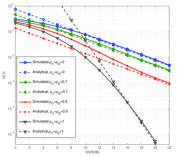
Figure 2: Analytical and simulated SER of $S_{1}$ with delay effect, with different $\rho_{f_{j}}$ and $\rho_{e}=1$, $N=4$.

In Fig. 2, we analyze the impact of delay on the SER performance without CEE , i.e., $\rho_{e}=1$. For simplicity, we assume $\rho_{f_{1}}=\rho_{f_{2}}=\rho_{f}$ and $N=4$. The figure reveals that the diversity order degrades to 1 once $\rho_{f}<1$ regardless of $N$. Although the diversity order is 1 once $\rho_{f}<1$, yet the coding gain is different for different $\rho_{f}$. Comparing the curves of $\rho_{f}=0.9$ and $\rho_{f}=0$, the coding gain gap between them is approximately 6dB in high SNR regime. Besides, the performance at moderate SNR is different for different $\rho_{f}$, i.e., greater $\rho_{f}$ has better performance at moderate SNR. For example, at moderate SNR, i.e., range from 8dB to 16dB, the slope of the SER curve of $\rho_{f}=0.9$ is greater than $1$, while the slope of $\rho_{f}=0$ at the same range is $1$. The performance at moderate SNR can be analyzed by the exact expression of SER and Maclaurian Series[22].

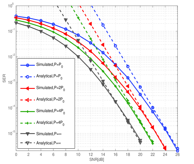
Figure 3: Analytical and simulated SER of $S_{1}$ with estimation error, with different $\rho_{e}$ and $\rho_{f_{1}}=\rho_{f_{2}}=1$, $N=4$.

In Fig. 3, we study the impact of CEE on the SER performance without delay, i.e., $\rho_{f}=1$ and $\rho_{e}={P}/\left({P+N_{0}}\right)$, where $P$ is the power of the training symbols[21]. $P$ can be greater than the power of the data symbols $P_{0}$ to obtain better performance of channel estimation, thus we simulate the situation of $P=P_{0},2P_{0},4P_{0}$ and $\infty$ ($P=\infty$ means no CEE), respectively. With CEE, the diversity order is invariant, which is the same as the number of relays. However, compared with the curve of $P=\infty$, there exists coding gain loss caused by CEE, and the loss could be reduced by increasing the power of training symbols $P_{0}$. As Fig. 3 illustrated, the coding gain loss in high SNR regime is about 5dB when $P=P_{0}$, but it reduces to 2dB when $P=4P_{0}$.

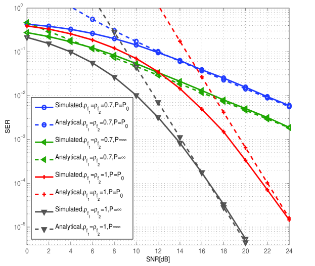
Figure 4: Analytical and simulated SER of $S_{1}$ with delay effect and estimation error, with different $\rho_{e}$ and $\rho_{f_{i}}$, $N=4$.

In Fig. 4, the joint effect of delay and channel estimation error is considered and compared with the cases of only delay effect, only CEE, and perfect CSI. The results also indicate that delay will result in the diversity order loss and the coding gain loss, and CEE will merely result in the coding gain loss. With both delay and CEE existing, the SER performance is the worst, which matches tightly with the analytical result in high SNR regime.

V Conclusions

In this paper, we analyzed the performance of bidirectional AF relay selection with imperfect CSI, i.e., delay effect and channel estimation error, and the asymptotic analytical expression of end-to-end SER was derived and verified by the computer simulation. Both analytical and simulated results indicate that delay effect results in the coding gain loss and the diversity order loss, and channel estimation error will merely cause the coding gain loss.

Appendix A
Proof of Lemma 1

At the case of $\rho_{f_{j}}=1$, we have $h_{t,ji}=h_{s,ji}$ by (1), and thus $\hat{h}_{t,ji}=\hat{h}_{s,ji}$, which is a special case of (7) when $\rho_{j}=1$ in Lemma 1.

At the case of $\rho_{f_{j}}<1$, by (1), (3) and (4), we have :

$$\hat{h}_{t,ji}=h_{t,ji}+e=\rho_{f_{j}}h_{s,ji}+\sqrt{1-\rho_{f_{j}}^{2}}\varepsilon_{j}+e=\rho_{f_{j}}\rho_{e}\hat{h}_{s,ji}+\rho_{f_{j}}d+\sqrt{1-\rho_{f_{j}}^{2}}\varepsilon_{j}+e~{},$$ (34)

where $d$, $\varepsilon_{j}$, and $e$ are independent zero mean complex-Gaussian RVs with variance of $\sigma_{D}^{2}$, $\sigma_{\varepsilon_{j}}^{2}$, and $\sigma_{e}^{2}$, respectively. Thus, $\rho_{f_{j}}d+\sqrt{1-\rho_{f_{j}}^{2}}\varepsilon_{j}+e$ is a zero mean complex-Gaussian RV with variance of $\rho_{f_{j}}^{2}\sigma_{D}^{2}+\left(1-\rho_{f_{j}}^{2}\right)\sigma_{\varepsilon_{j}}^{2}+\sigma_{e}^{2}$ , which can be simplified into $\left(1-\rho_{f_{j}}^{2}\rho_{e}^{2}\right)\sigma_{\hat{h}_{t,ji}}^{2}$ by the relationship of variances (5),(6). Then, $\rho_{f_{j}}d+\sqrt{1-\rho_{f_{j}}^{2}}\varepsilon_{j}+e$ can be written as $\sqrt{1-\rho_{f_{j}}^{2}\rho_{e}^{2}}v_{j}$ , where $v_{j}$ is an independent RV with zero mean and variance of $\sigma_{\hat{h}_{t,ji}}^{2}$. Defining $\rho_{j}=\rho_{e}\rho_{f_{j}}$ , formula (7) in Lemma 1 is proved. Thus, $\hat{h}_{t,ji}$ and $\hat{h}_{s,ji}$ are jointly complex-Gaussian, and $\hat{\gamma}_{t,ji}=\left|\hat{h}_{t,ji}\right|^{2}$ and $\hat{\gamma}_{s,ji}=\left|\hat{h}_{s,ji}\right|^{2}$ are correlated exponential distributions, then the joint PDF $f_{\hat{\gamma}_{t,ji},\hat{\gamma}_{s,ji}}\left({y,x}\right)$ is given by[25]:

$$f_{\hat{\gamma}_{t,ji},\hat{\gamma}_{s,ji}}\left({y,x}\right)=\frac{1}{{\left({1-\rho_{j}^{2}}\right)\sigma_{\hat{h}}^{4}}}\exp\left({-\frac{{x+y}}{{\left({1-\rho_{j}^{2}}\right)\sigma_{\hat{h}}^{2}}}}\right)I_{0}\left({\frac{{2\sqrt{\rho_{j}^{2}xy}}}{{\left({1-\rho_{j}^{2}}\right)\sigma_{\hat{h}}^{2}}}}\right)~{}.$$ (35)

And now, the conditional probability of (9) in Lemma 1 can be proved by[26]:

$$f_{\hat{\gamma}_{t,ji}|\hat{\gamma}_{s,ji}}\left({y|x}\right)=\frac{f_{\hat{\gamma}_{t,ji},\hat{\gamma}_{s,ji}}\left({y,x}\right)}{f_{\hat{\gamma}_{s,ji}}\left(x\right)}~{},$$ (36)

where $f_{\hat{\gamma}_{s,ji}}\left(x\right)=\exp\left({-x/\sigma_{\hat{h}}^{2}}\right)/\sigma_{\hat{h}}^{2}$ .

Appendix B
Proof of Theorem 1

V-A distribution of $\hat{\gamma}_{s,1k}$ and $\hat{\gamma}_{s,2k}$

Following the similar steps of [14] , the CDF of $\hat{\gamma}_{s,1k}$ can be expressed as :

$$F_{\hat{\gamma}_{s,1k}}\left(x\right) \buildrel\left(a\right)\over{=}N\Pr\left\{{\hat{\gamma}_{s,1i}<x,k=i}\right\}$$ (37)

$$\buildrel\left(b\right)\over{=}N\int\limits_{0}^{x}{f_{\hat{\gamma}_{s,1i}}\left(y\right)}\Pr\left\{{\hat{\gamma}_{s,1i}\leq\hat{\gamma}_{s,2i}|\hat{\gamma}_{s,1i}=y}\right\}\Pr\left\{{k=i|\hat{\gamma}_{s,1i}\leq\hat{\gamma}_{s,2i},\hat{\gamma}_{s,1i}=y}\right\}dy$$

$$+N\int\limits_{0}^{x}{f_{\hat{\gamma}_{s,1i}}(y)}\Pr\left\{{\hat{\gamma}_{s,1i}>\hat{\gamma}_{s,2i}|\hat{\gamma}_{s,1i}=y}\right\}\Pr\left\{{k=i|\hat{\gamma}_{s,1i}>\hat{\gamma}_{s,2i},\hat{\gamma}_{s,1i}=y}\right\}dy~{}$$

where (a) in (37) is satisfied due to the symmetry among the $N$ end-to-end paths, and (b) is satisfied by dividing the union event into two disjoint events, i.e., $\hat{\gamma}_{s,1i}>\hat{\gamma}_{s,2i}$ and $\hat{\gamma}_{s,1i}\leq\hat{\gamma}_{s,2i}$. According to the selection criterion (11) and order statistics of independent RVs[27]: $\Pr\big{\{}{\min\big{(}{x1,x2}\big{)}\leq z}\big{\}}=1-\left(1-F_{x_{1}}\left(z\right)\right)\left(1-F_{x_{2}}\left(z\right)\right)$, and the fact that $F_{\hat{\gamma}_{s,1i}}\left(z\right)=F_{\hat{\gamma}_{s,2i}}\left(z\right)=1-\exp\left({-z/\sigma_{\hat{h}}^{2}}\right)$, we have

$$\Pr\left\{{k=i|\hat{\gamma}_{s,1i}\leq\hat{\gamma}_{s,2i},\hat{\gamma}_{s,1i}=y}\right\}=\prod\limits_{p\neq i}{\Pr}\left\{{\min\left({\hat{\gamma}_{s,1i},\hat{\gamma}_{s,2i}}\right)\leq y}\right\}=\left({1-\exp\left({-\frac{2y}{\sigma_{\hat{h}}^{2}}}\right)}\right)^{N-1}~{}.$$ (38)

Similarly, the conditional probability $\Pr\left\{{k=i|\hat{\gamma}_{s,1i}>\hat{\gamma}_{s,2i},\hat{\gamma}_{s,1i}=y}\right\}$ can be achieved. Therefore, substituting (38) into (37), $F_{\hat{\gamma}_{s,1k}}\left(x\right)$ can be written as :

$$F_{\hat{\gamma}_{s,1k}}\left(x\right) =~{}N\int_{0}^{x}{\frac{1}{{\sigma_{\hat{h}}^{2}}}\exp\left({-\frac{y}{{\sigma_{\hat{h}}^{2}}}}\right)}\left({\int_{0}^{y}{\frac{1}{{\sigma_{\hat{h}}^{2}}}\exp\left({-\frac{z}{{\sigma_{\hat{h}}^{2}}}}\right)}\left({1-\exp\left({-\frac{{2z}}{{\sigma_{\hat{h}}^{2}}}}\right)}\right)^{N-1}dz}\right)dy$$ (39)

$$+~{}N\int_{0}^{x}{\frac{1}{{\sigma_{\hat{h}}^{2}}}\exp\left({-\frac{y}{{\sigma_{\hat{h}}^{2}}}}\right)}\left({\int_{y}^{\infty}{\frac{1}{{\sigma_{\hat{h}}^{2}}}\exp\left({-\frac{z}{{\sigma_{\hat{h}}^{2}}}}\right)}dz}\right)\left({1-\exp\left({-\frac{{2y}}{{\sigma_{\hat{h}}^{2}}}}\right)}\right)^{N-1}dy~{}.$$

Applying binomial expansion $\left({1-x}\right)^{N}=\sum\nolimits_{k=0}^{N}{\binom{N}{k}}\left({-1}\right)^{k}x^{k}$ and $N\sum\nolimits_{n=0}^{N-1}\binom{N-1}{n}{{\left({-1}\right)^{n}}}/\left({{n+1}}\right)=1$ in [24, (0.155.1)], $F_{\hat{\gamma}_{s,1k}}\left(x\right)$ can be rewritten as :

$$F_{\hat{\gamma}_{s,1k}}\left(x\right)=1- N\sum\limits_{n=0}^{N-1}\binom{N-1}{n}\frac{{\left({-1}\right)^{n}}}{{2n+1}}\left[\exp\left({-\frac{x}{{\sigma_{\hat{h}}^{2}}}}\right)+\frac{n}{{n+1}}\exp\left({-\frac{{2\left({n+1}\right)x}}{{\sigma_{\hat{h}}^{2}}}}\right)\right]~{},$$ (40)

where $\sigma_{\hat{h}}^{2}=\rho_{e}^{-1}$, and it can be proved similarly that the CDF of $\hat{\gamma}_{s,1k}$ have the same form, and their PDFs can be obtained by differentiating the CDFs.

V-B distribution of $\gamma_{1}$

At the case of $\rho_{f_{1}}<1$ and $\rho_{f_{2}}<1$, and by Lemma 1 and $\int\limits_{0}^{\infty}{\exp\left(-\alpha x\right)I_{0}\left(\beta\sqrt{x}\right)}dx=\left({1}/{\alpha}\right)\exp\left({{\beta^{2}}}/\left({{4\alpha}}\right)\right)$ in [24, (6.614.3)], we have :

$$f_{\hat{\gamma}_{t,1k}}\left(x\right) =N\sum\limits_{n=0}^{N-1}{\left({-1}\right)^{n}\binom{N-1}{n}}\frac{1}{{2n+1}}\left[\frac{{\exp\left({-x/\sigma_{\hat{h}}^{2}}\right)}}{{\sigma_{\hat{h}}^{2}}}\right.$$ (41)

$$\left.+\frac{{2n/\sigma_{\hat{h}}^{2}}}{{\left({2n+1}\right)\left({1-\rho_{1}^{2}}\right)+1}}\exp\left({-\frac{{2\left({n+1}\right)x/\sigma_{\hat{h}}^{2}}}{{\left({2n+1}\right)\left({1-\rho_{1}^{2}}\right)+1}}}\right)\right]~{}.$$

The CDF of $\hat{\gamma}_{t,1k}$ can be obtained by integrating the PDF, and the distribution of $\hat{\gamma}_{t,2k}$ can be obtained by substituting $\rho_{1}$ with $\rho_{2}$. Let $\Omega_{1}$ and $\Omega_{2}$ represent $\tilde{a}\hat{\gamma}_{t,1k}$, and $\tilde{b}\hat{\gamma}_{t,2k}$ respectively, and the distribution of $\Omega_{1}$ and $\Omega_{2}$ can be obtained by $f_{Y}\left(y\right)=\left({1}/{m}\right)f_{X}\left({x}/{m}\right)$, and $F_{Y}\left(y\right)=F_{X}\left({x}/{m}\right)$ when $Y=mX\left(m>0\right)$[26]. Thus, the CDF of $\gamma_{1}$ can be written as :

$$F_{\gamma_{1}}\left(z\right) =\Pr\left\{{\frac{{\Omega_{1}\Omega_{2}}}{{\Omega_{1}+\Omega_{2}}}<z}\right\}$$ (42)

$$=\Pr\left\{{\left({\Omega_{2}-z}\right)\Omega_{1}<z\Omega_{2},\Omega_{2}>z}\right\}+\Pr\left\{{\left({\Omega_{2}-z}\right)\Omega_{1}<z\Omega_{2},\Omega_{2}\leq z}\right\}$$

$$=\int_{z}^{\infty}{F_{\Omega_{1}}\left({\frac{{zx}}{{x-z}}}\right)}f_{\Omega_{2}}\left(x\right)dx+\int_{0}^{z}{\left[{1-F_{\Omega_{1}}\left({\frac{{zx}}{{x-z}}}\right)}\right]}f_{\Omega_{2}}\left(x\right)dx$$

$$=1-\int\limits_{0}^{\infty}{f_{\Omega_{2}}\left({x+z}\right)\left[{1-F_{\Omega_{1}}\left({z+\frac{{z^{2}}}{x}}\right)}\right]}dx$$

Substituting $\int\limits_{0}^{\infty}{\exp\left(-mx-nx^{-1}\right)}dx=2\sqrt{{n}/{m}}K_{1}\left(2\sqrt{mn}\right)$ in [24, (3.324)] into (42), Theorem 2 can be proved when using $N\sum\nolimits_{n=0}^{N-1}{\binom{N-1}{n}{{\left({-1}\right)^{n}}}/\left({{n+1}}\right)}=1$ in [24, (0.155.1)].

At the case of $\rho_{f_{1}}=1$ or $\rho_{f_{2}}=1$, it can be proved in a similar way that the CDF of $\gamma_{1}$ can also be expressed as the formula (23) in Theorem 1.

Appendix C
Proof of Theorem 2

In high SNR regime ($\psi_{r}$,$\psi_{s}$ $\to$ $\infty$), $\rho_{e}\to 1$ and $a,b\to 0$. By applying the Bessel function approximation for small $x\to 0$, $K_{1}\left(x\right)\approx{1}/{x}$[23] in Theorem 1, we have :

$$F_{\gamma_{1}}\left(z\right) \approx 1-N^{2}\sum\limits_{m=0}^{N-1}{\sum\limits_{n=0}^{N-1}{\left({-1}\right)^{m+n}\binom{N-1}{m}}}\binom{N-1}{n}\frac{1}{{2m+1}}\frac{1}{{2n+1}}$$ (43)

$$\times\bigg{[}\exp\left({-\left({a+b}\right)z}\right)+\frac{n}{{n+1}}\exp\left({-\left({\frac{{2\left({n+1}\right)a}}{{\left({2n+1}\right)\left({1-\rho_{1}}\right)+1}}+b}\right)z}\right)$$

$$+\frac{m}{{m+1}}\exp\left({-\left({a+\frac{{2\left({m+1}\right)b}}{{\left({2m+1}\right)\left({1-\rho_{2}}\right)+1}}}\right)z}\right)$$

$$+\frac{m}{{m+1}}\frac{n}{{n+1}}\exp\left({-\left({\frac{{2\left({n+1}\right)a}}{{\left({2n+1}\right)\left({1-\rho_{1}}\right)+1}}+\frac{{2\left({m+1}\right)b}}{{\left({2m+1}\right)\left({1-\rho_{2}}\right)+1}}}\right)z}\right)\bigg{]}~{}.$$

At the case of $\rho_{f_{1}}=\rho_{f_{2}}=1$, $F_{\gamma_{1}}\left(z\right)$ can be rewritten as :

$$F_{\gamma_{1}}\left(z\right) =1-N\sum\limits_{n=0}^{N-1}{\left({-1}\right)^{n}}\binom{N-1}{n}\frac{1}{{2n+1}}\left[{\exp\left({-az}\right)+\frac{n}{{n+1}}\exp\left({-2\left({n+1}\right)az}\right)}\right]$$ (44)

$$\times N\sum\limits_{m=0}^{N-1}{\left({-1}\right)^{m}}\binom{N-1}{m}\frac{1}{{2m+1}}\left[{\exp\left({-bz}\right)+\frac{m}{{m+1}}\exp\left({-2\left({m+1}\right)bz}\right)}\right]~{}.$$

Furthermore, we have :

$$N\sum\limits_{n=0}^{N-1}{\left({-1}\right)^{n}}\binom{N-1}{n}\frac{1}{{2n+1}}\left[{\exp\left({-az}\right)+\frac{n}{{n+1}}\exp\left({-2\left({n+1}\right)az}\right)}\right]$$ (45)

$$=~{} N\sum\limits_{n=0}^{N-1}{\left({-1}\right)^{n}}\binom{N-1}{n}\frac{1}{{n+1}}{\exp\left({-2\left({n+1}\right)az}\right)}$$

$$+~{} N\sum\limits_{n=0}^{N-1}{\left({-1}\right)^{n}}\binom{N-1}{n}\frac{1}{{2n+1}}\left[\exp\left({-az}\right)-\exp\left({-2\left({n+1}\right)az}\right)\right]$$

$$\buildrel\left(a\right)\over{=}~{} 1-\left[{1-\exp\left({-2az}\right)}\right]^{N}-\exp\left({-az}\right)\left[{N\sum\limits_{n=0}^{N-1}{\left({-1}\right)^{n}}\binom{N-1}{n}\frac{1}{{2n+1}}\left({1-\exp\left({-\left({2n+1}\right)az}\right)}\right)}\right]$$

$$\buildrel\left(b\right)\over{=}~{} 1-\left[{-\sum\limits_{p=1}^{\infty}{\frac{{\left({-2az}\right)^{p}}}{{p!}}}}\right]^{N}-\sum\limits_{p=0}^{\infty}{\frac{{\left({-az}\right)^{p}}}{{p!}}}\left[N\sum\limits_{n=0}^{N-1}{\left({-1}\right)^{n}}\binom{N-1}{n}\sum\limits_{p=1}^{\infty}{\left(2n+1\right)^{p-1}\frac{{\left({-az}\right)^{p}}}{{p!}}}\right]$$

$$\buildrel\left(c\right)\over{=}~{} 1-\frac{1}{2}\left(2az\right)^{N}+o((az)^{N})~{},$$

where (a) in (45) is achieved by the fact that $\binom{N-1}{n}\frac{N}{n+1}=\binom{N}{n+1}$ and $\left({1-x}\right)^{N}=\sum\nolimits_{k=0}^{N}{\binom{N}{k}}\left({-1}\right)^{k}x^{k}$; (b) is achieved by Maclaurian Series of $\exp\left(x\right)=\sum\nolimits_{p=0}^{\infty}\left(x^{p}\right)/\left(p!\right)$; (c) is achieved by $\sum\nolimits_{k=0}^{N}{\left({-1}\right)^{k}\binom{N}{n}k^{n-1}}=0,\left({1\leq n\leq N}\right)$ in [24, (0.154.3)]. Therefore,

$$F_{\gamma_{1}}\left(z\right)\approx[\frac{1}{2}\left(2a\right)^{N}+\frac{1}{2}\left(2b\right)^{N}]z^{N}~{}.$$ (46)

Finally, (31) in Theorem 2 is proved by (22),  (29), (46), and $\int\limits_{0}^{\infty}{t^{2N}}\exp\left(-{t^{2}}/{2}\right)dt={2^{\left(N-{1}/{2}\right)}}\Gamma\left({1}/{2}+N\right)=\sqrt{{\pi}/{2}}{{\left(2N\right)!}}/{{\left(2^{N}N!\right)}}$ in [24, (3.326.2)], where $\Gamma\left(\cdot\right)$ is Gamma function[23].

At the case of $\rho_{f_{1}}<1$ or $\rho_{f_{2}}<1$, by $\exp\left(x\right)\approx 1+x$, we similarly have :

$$F_{\gamma_{1}}\left(z\right)\approx azN\sum\limits_{n=0}^{N-1}{\left({-1}\right)^{n}}\binom{N-1}{n}\frac{{2-\rho_{1}}}{{\left({2n+1}\right)\left({1-\rho_{1}}\right)+1}}$$ (47)

$$+ bzN\sum\limits_{m=0}^{N-1}{\left({-1}\right)^{m}}\binom{N-1}{m}\frac{{2-\rho_{2}}}{{\left({2m+1}\right)\left({1-\rho_{2}}\right)+1}}~{}.$$

Then, (32) in Theorem 2 is proved by (22) and (29).

Figure 1: Analytical and simulated SER with perfect CSI, with different $N$, $\rho_{f_{1}}=\rho_{f_{2}}=1$ and $\rho_{e}=1$.

References

• [1] S. Katti, H. Rahul, W. Hu, D. Katabi, M. Medard, and J. Crowcroft, “Xors in the air: Practical wireless network coding,” IEEE/ACM Transactions on Networking, vol. 16, no. 3, pp. 497–510, Jun. 2008.
• [2] P. Popovski and H. Yomo, “Wireless network coding by amplify-and-forward for bi-directional traffic flows,” IEEE Communication Letters, vol. 11, no. 1, pp. 16–18, Jan. 2007.
• [3] R. H. Y. Louie, Y. Li,  and B. Vucetic, “Practical physical layer network coding for two-way relay channels: Performance analysis and comparison,” IEEE Transactions on Wireless Communications, vol. 9, no. 2, pp. 764–777, Feb. 2010.
• [4] A. Bletsas, A. Khisti, D. P. Reed, and A. Lippman, “A simple Cooperative diversity method based on network path selection,” IEEE Journal on Selected Areas in Communications, vol. 24, no. 3, pp. 659–672, Mar. 2006.
• [5] A. S. Ibrahim, A. K. Sadek, W. Su, and K. J. R. Liu, “Cooperative communications with relay-selection: When to cooperate and whom to cooperate with?,” IEEE Transactions on Wireless Communications, vol. 7, no. 7, pp. 2814–2827, Jul. 2008.
• [6] X. Zhang and Y. Gong, “Adaptive power allocation in two-way amplify-and-forward relay networks,” in Proceedings of IEEE International Conference on Communication, Jun. 2009.
• [7] K. Hwang, Y. Ko, and M.-S. Alouini, “Performance bounds for two-Way amplify-and-forward relaying based on relay path selection,” in Proceedings of Vehicular Technology Conference, Apr. 2009.
• [8] L. Song, G. Hong, B. Jiao, and M. Debbah, “Joint relay selection and analog network coding using differential modulation in two-way relay channels,” IEEE Transactions on Vehicular Technology, vol. 59, no. 6, pp. 2932–2939, Jul. 2010.
• [9] L. Song, “Relay selection for two-way relaying with amplify-and-forward protocols,” IEEE Transactions on Vehicular Technology, vol. 60, no. 4, pp. 1954–1959, May 2011.
• [10] Y. Jing, “A relay selection scheme for two-way amplify-and-forward relay networks,” in Proceedings of International Conference of Wireless Communication and Signal Process, Nov. 2009.
• [11] H. X. Nguyen, H. H. Nguyen, and T. Le-Ngoc, “Diversity analysis of relay selection schemes for two-way wireless relay networks,” in Wireless Personal Communication, Jan. 2010.
• [12] M. Torabi and D. Haccoun, “Capacity analysis of opportunistic relaying in cooperative systems with outdated channel information,” IEEE Communications Letters, vol. PP, no. 99, pp. 1–3, Nov. 2010.
• [13] H. A. Suraweera, M. Soysa, C. Tellambura, and H. K. Garg, “Performance analysis of partial relay selection with feedback delay,” IEEE Signal Processing Letters , vol. 17, no. 6, pp. 531–534, Jun. 2010.
• [14] D. S. Michalopoulos, H. A. Suraweera, G. K. Karagiannidis , and R. Schober, “Amplify-and-forward relay selection with outdated channel state information,” in Proceedings of IEEE Global Telecommunications Conference, Dec. 2010.
• [15] M. Seyfi, S. Muhaidat, and J. Liang, “Amplify-and-forward selection cooperation with channel estimation error,” in Proceedings of IEEE Global Telecommunications Conference, Dec. 2010.
• [16] S. Han, S. Ahn, E. Oh, and D. Hong, “Effect of channel estimation error on BER performance in cooperative transmission,” IEEE Transactions on Vehicular Technology, vol. 58, no. 4, pp. 2083–2088, May 2009.
• [17] B. Gedik and M. Uysal, “Impact of imperfect channel estimation on the performance of amplify-and-forward relaying,” IEEE Transactions on Wireless Communications, vol. 8, no. 3, pp. 1468–1479, Mar. 2009.
• [18] Z. Ding and K. K. Leung, “Impact of imperfect channel state information on bi-directional communications with relay selection,” IEEE Transactions on Signal Processing, vol. 59, no. 11, pp. 5657–5662, Nov. 2011.
• [19] T. Yoo and A. Goldsmith, “Capacity and power allocation for fading MIMO channels with channel estimation error,” IEEE Transactions on Information Theory, vol. 52, no. 5, pp. 2203–2214, May 2006.
• [20] F. Gao, R. Zhang, and Y. Liang, “Optimal channel estimation and training design for two-way relay networks,” IEEE Transactions on Communications, vol. 57, no. 10, pp. 3024–3033, Oct. 2009.
• [21] T. R. Ramya and S. Bhashyam, “Using delayed feedback for antenna selection in MIMO systems,” IEEE Transactions on Wireless Communications, vol. 8, no. 12, pp. 6059–6067, Dec. 2009.
• [22] Z. Wang and G. B. Giannakis, “A simple and general parameterization quantifying performance in fading channels,” IEEE Transactions on Communications, vol. 51, no. 8, pp. 1389–1398, Aug. 2003.
• [23] M. Abramowitz and I. A. Stegun, Handbook of mathematical functions with formulas, graphs, and mathematical tables, 9th ed. NewYork: Dover, 1970.
• [24] I. S. Gradshteyn and I. M. Ryzhik, Table of integals, series, and products, 5th Edition, Academic Press, 1994.
• [25] M. K. Simon and M.-S. Alouini, Digital Communication over Fading Channels. John Wiley $\&$ Sons, Inc., 2000.
• [26] A. Paoulis, S. U. Pialli, Probability, Random Variables and Stochastic Processes. 4th Edition, McGraw-Hill, 2002.
• [27] H. A. David, Order Statistics. Jonh Wiley $\&$ Sons, Inc., 1970.
Refer to caption