Spin-polarized current effect on antiferromagnet magnetization in a ferromagnet–antiferromagnet nanojunction: Theory and simulation

Abstract

Spin-polarized current effect is studied on the static and dynamic magnetization of the antiferromagnet in a ferromagnet–antiferromagnet nanojunction. The macrospin approximation is generalized to antiferromagnets. Canted antiferromagnetic configuration and resulting magnetic moment are induced by an external magnetic field. The resonance frequency and damping are calculated, as well as the threshold current density corresponding to instability appearance. A possibility is shown of generating low-damping magnetization oscillations in terahertz range. The fluctuation effect is discussed on the canted antiferromagnetic configuration. Numerical simulation is carried out of the magnetization dynamics of the antiferromagnetic layer in the nanojunction with spin-polarized current. Outside the instability range, the simulation results coincide completely with analytical calculations using linear approximation. In the instability range, undamped oscillations occur of the longitudinal and transverse magnetization components.

1 Introduction

The discovery of the spin transfer torque effect in ferromagnetic junctions under spin-polarized current [1, 2] has stimulated a number of works in which such effects were observed as switching the junction magnetic configuration [3], spin wave generation [4], current-driven motion of magnetic domain walls [5], modification of ferromagnetic resonance [6], etc. It is well known that the spin torque transfer from spin-polarized electrons to lattice leads to appearance of a negative damping. At some current density, this negative damping overcomes the positive (Gilbert) damping with occurring instability of the original magnetic configuration. The corresponding current density is high enough, of the order of $10^{7}$ A/cm². This, naturally, stimulates attempts to lower this threshold. Various ways were proposed, such as using magnetic semiconductors [7], in which the threshold current density can be lower down to $10^{5}$–$10^{6}$ A/cm² because of their low saturation magnetization. However, using of such materials requires, as a rule, low temperatures because of low Curie temperature. Besides, the ferromagnetic resonance frequency is rather low in this case.

In connection with these difficulties, the other approaches were proposed, based on high spin injection [8] or joint action of external magnetic field and spin-polarized current [9, 10]. It seems promising, also, using magnetic junction of ferromagnet–antiferromagnet type, in which the ferromagnet (FM) acts as an injector of spin-polarized electrons. The antiferromagnetic (AFM) layer, in which the magnetic sublattices are canted by external magnetic field, may have very low magnetization that promotes low threshold [11]. The AFM resonance frequency may be both low and high reaching $10^{12}$ s^-1, i.e. terahertz (THz) range. However, investigation and application of THz resonances is prevented because of their large damping. Such a damping in ferromagnetic junctions can be suppressed, as mentioned above, by means of spin-polarized current. The question arises about possibility of such a suppression in FM/AFM junctions. Note, that this problem has been paid attention of a number of authors [12]–[21].

Another interesting feature of the FM/AFM junctions with spin-polarized current is the possibility of canting the AFM structure by spin-polarized current without magnetic field.

2 The equations of motion

Let us consider a FM/AFM junction (Fig. 1) with current flowing perpendicular to layers, along $x$ axis. An ultrathin spacer layer is placed between the FM and AFM layers to prevent direct exchange coupling between the layers. An external magnetic field is parallel to the FM magnetization and lies in the layer plane $yz$. The simplest AFM model is used with two equivalent sublattices.

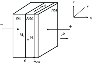
Figure 1: Scheme of the ferromagnet (FM)–antiferromagnet (AFM) junction; NM being a nonmagnetic layer. The main vector directions are shown.

The AFM energy (per unit area), with uniform and nonuniform exchange, anisotropy, external magnetic field, and the sd exchange interaction of the conduction electrons with the magnetic lattice taking into account, takes the form [22]

$$W=\int_{0}^{L_{AFM}}\,dx\biggl{\{}\Lambda(\mathbf{M}_{1}\cdot\mathbf{M}_{2})+\frac{1}{2}\alpha\left\{\left(\frac{\partial\mathbf{M}_{1}}{\partial x}\right)^{2}+\left(\frac{\partial\mathbf{M}_{2}}{\partial x}\right)^{2}\right\}$$

$$+\alpha^{\prime}\left(\frac{\partial\mathbf{M}_{1}}{\partial x}\cdot\frac{\partial\mathbf{M}_{2}}{\partial x}\right)-\frac{1}{2}\beta\left\{(\mathbf{M}_{1}\cdot\mathbf{n})^{2}+(\mathbf{M}_{2}\cdot\mathbf{n})^{2}\right\}$$

$$-\beta^{\prime}(\mathbf{M}_{1}\cdot\mathbf{n})(\mathbf{M}_{2}\cdot\mathbf{n})-((\mathbf{M}_{1}+\mathbf{M}_{2})\cdot\mathbf{H})$$

$$-\alpha_{sd}((\mathbf{M}_{1}+\mathbf{M}_{2})\cdot\mathbf{m})\biggr{\}},$$ (1)

where $\mathbf{M}_{1},\,\mathbf{M}_{2}$ are the sublattice magnetization vectors, $\Lambda$ is the uniform exchange constant, $\alpha,\,\alpha^{\prime}$ are the intra- and inter-sublattice nonuniform exchange constants, respectively, $\beta,\,\beta^{\prime}$ are the corresponding anisotropy constants, $\mathbf{n}$ is the unit vector along the anisotropy axis, $\mathbf{H}$ is the external magnetic field, $\mathbf{m}$ is the conduction electron magnetization, $\alpha_{sd}$ is the dimensionless sd exchange interaction constant. We do not include demagnetization term because its contribution is small compared to the uniform exchange. The integral is taken over the AFM layer thickness $L_{AFM}$. We are interested in the spin-polarized current effect on the AFM layer, so we consider a case of perfect FM injector with pinned lattice magnetization and without disturbance of the electron spin equilibrium, that allows to not include the FM layer energy in Eq. (2).

Two mechanisms are known of the spin-polarized current effect on the magnetic lattice, namely, spin transfer torque (STT) [1, 2] and an alternative mechanism [23, 24] due to the spin injection and appearance of nonequilibrium population of the spin subbands in the collector layer (this is the AFM layer, in our case). In the case of antiparallel relative orientation of the injector and collector magnetization vectors, such a state becomes energetically unfavorable at high enough current density, so that the antiparallel configuration switches to parallel one (such a process in FM junction is considered in detail in review [25]). The latter mechanism is described with the sd exchange term in Eq. (2). As to the former mechanism, it is of dissipative character (it leads to negative damping), so that it is taken into account by the boundary conditions (see below), not the Hamiltonian.

The equations of the sublattice motion with damping taking into account take the form

$$\frac{\partial\mathbf{M}_{i}}{\partial t}-\frac{\kappa}{M_{0}}\left[\mathbf{M}_{i}\times\frac{\partial\mathbf{M}_{i}}{\partial t}\right]+\gamma\left[\mathbf{M}_{i}\times\mathbf{H}_{eff}^{(i)}\right]=0\quad(i=1,\,2),$$ (2)

where $M_{0}$ is the sublattice magnetization, $\kappa$ is the damping constant,

$$\mathbf{H}_{eff}^{(i)}=-\frac{\delta W}{\delta\mathbf{M}_{i}}\quad(i=1,\,2)$$ (3)

are the effective fields acting on the corresponding sublattices.

From Eqs. (2)–(3) the equations are obtained for the total magnetization $\mathbf{M}=\mathbf{M}_{1}+\mathbf{M}_{2}$ and antiferromagnetism vector $\mathbf{L}=\mathbf{M}_{1}-\mathbf{M}_{2}$:

$$\frac{\partial\mathbf{M}}{\partial t}-\frac{1}{2}\frac{\kappa}{M_{0}}\left\{\left[\mathbf{M}\times\frac{\partial\mathbf{M}}{\partial t}\right]+\left[\mathbf{L}\times\frac{\partial\mathbf{L}}{\partial t}\right]\right\}$$

$$+\gamma\left[\mathbf{M}\times\mathbf{H}\right]+\gamma\left[\mathbf{M}\times\mathbf{H}_{sd}\right]$$

$$+\frac{1}{2}\gamma(\beta+\beta^{\prime})(\mathbf{M}\cdot\mathbf{n})[\mathbf{M}\times\mathbf{n}]+\frac{1}{2}\gamma(\beta-\beta^{\prime})(\mathbf{L}\cdot\mathbf{n})[\mathbf{L}\times\mathbf{n}]$$

$$+\frac{1}{2}\gamma(\alpha+\alpha^{\prime})\left[\mathbf{M}\times\frac{\partial^{2}\mathbf{M}}{\partial x^{2}}\right]+\frac{1}{2}\gamma(\alpha-\alpha^{\prime})\left[\mathbf{L}\times\frac{\partial^{2}\mathbf{L}}{\partial x^{2}}\right]=0,$$ (4)

$$\frac{\partial\mathbf{L}}{\partial t}-\frac{1}{2}\frac{\kappa}{M_{0}}\left\{\left[\mathbf{L}\times\frac{\partial\mathbf{M}}{\partial t}\right]+\left[\mathbf{M}\times\frac{\partial\mathbf{L}}{\partial t}\right]\right\}$$

$$+\gamma\left[\mathbf{L}\times\mathbf{H}\right]+\gamma\left[\mathbf{L}\times\mathbf{H}_{sd}\right]-\gamma\Lambda\left[\mathbf{L}\times\mathbf{M}\right]$$

$$+\frac{1}{2}\gamma(\beta+\beta^{\prime})(\mathbf{M}\cdot\mathbf{n})[\mathbf{L}\times\mathbf{n}]+\frac{1}{2}\gamma(\beta-\beta^{\prime})(\mathbf{L}\cdot\mathbf{n})[\mathbf{M}\times\mathbf{n}]$$

$$+\frac{1}{2}\gamma(\alpha+\alpha^{\prime})\left[\mathbf{L}\times\frac{\partial^{2}\mathbf{M}}{\partial x^{2}}\right]+\frac{1}{2}\gamma(\alpha-\alpha^{\prime})\left[\mathbf{M}\times\frac{\partial^{2}\mathbf{L}}{\partial x^{2}}\right]=0,$$ (5)

where

$$\mathbf{H}_{sd}(x)=\frac{\delta}{\delta\mathbf{M}(x)}\int_{0}^{L_{AFM}}\left(\mathbf{M}(x^{\prime})\cdot\mathbf{m}(x^{\prime})\right)\,dx^{\prime}$$ (6)

is the effective field due to sd exchange interaction. This field determines the spin injection contribution to the interaction of the conduction electrons with the antiferromagnet lattice.

To find $\mathbf{H}_{sd}(x)$ field, the conduction electron magnetization $\mathbf{m}(x)$ is to be calculated. The details of such calculations are presented in our preceding papers [26, 9]. Here we adduce the result for the case, where the antiferromagnet layer thickness $L_{AFM}$ is small compared to the spin diffusion length $l$ with the current flow direction corresponding to the electron flux from FM to AFM:

$$\mathbf{m}=(\overline{m}+\Delta m)\hat{\mathbf{M}},\quad\Delta m=\frac{\mu_{B}\tau Qj}{eL_{AFM}}\left(\hat{\mathbf{M}}(0)\cdot\hat{\mathbf{M}}_{F}\right),$$ (7)

where $\overline{m}$ is the equilibrium (in absence of current) electron magnetization, $\Delta m$ is the nonequilibrium increment due to current, $\hat{\mathbf{M}}=\mathbf{M}/|\mathbf{M}|$ is the unit vector along the AFM magnetization, $\hat{\mathbf{M}}_{F}$ is the similar vector for FM, $\mu_{B}$ is the Bohr magneton, $e$ is the electron charge, $\tau$ is the electron spin relaxation time, $j$ is the current density.

It should have in mind in varying the integral (6), that the electron magnetization $\mathbf{m}$ depends on the vector $\mathbf{M}$ orientation relative to the FM magnetization vector $\mathbf{M}_{F}$. From Eqs. (6) and (7) we have [9]

$$\mathbf{H}_{sd}=\alpha_{sd}\overline{m}\hat{\mathbf{M}}+\alpha_{sd}\displaystyle\frac{\mu_{B}\tau Qj}{eL_{AFM}}\left(\hat{\mathbf{M}}(0)\cdot\hat{\mathbf{M}}_{F}\right)\hat{\mathbf{M}}$$ (8)

$$+\alpha_{sd}\displaystyle\frac{\mu_{B}\tau Qj}{e}\hat{\mathbf{M}}_{F}\delta(x-0).$$

By substitution (8) into (2) and (2), we obtain

$$\frac{\partial\mathbf{M}}{\partial t}-\frac{1}{2}\frac{\kappa}{M_{0}}\left\{\left[\mathbf{M}\times\frac{\partial\mathbf{M}}{\partial t}\right]+\left[\mathbf{L}\times\frac{\partial\mathbf{L}}{\partial t}\right]\right\}$$

$$+\gamma\left[\mathbf{M}\times\mathbf{H}\right]+\gamma\alpha_{sd}\frac{\mu_{B}\tau Qj}{e}\left[\mathbf{M}\times\hat{\mathbf{M}}_{F}\right]\delta(x-0)$$

$$+\frac{1}{2}\gamma(\beta+\beta^{\prime})(\mathbf{M}\cdot\mathbf{n})[\mathbf{M}\times\mathbf{n}]+\frac{1}{2}\gamma(\beta-\beta^{\prime})(\mathbf{L}\cdot\mathbf{n})[\mathbf{L}\times\mathbf{n}]$$

$$+\frac{1}{2}\gamma(\alpha+\alpha^{\prime})\left[\mathbf{M}\times\frac{\partial^{2}\mathbf{M}}{\partial x^{2}}\right]+\frac{1}{2}\gamma(\alpha-\alpha^{\prime})\left[\mathbf{L}\times\frac{\partial^{2}\mathbf{L}}{\partial x^{2}}\right]=0,$$ (9)

$$\frac{\partial\mathbf{L}}{\partial t}-\frac{1}{2}\frac{\kappa}{M_{0}}\left\{\left[\mathbf{L}\times\frac{\partial\mathbf{M}}{\partial t}\right]+\left[\mathbf{M}\times\frac{\partial\mathbf{L}}{\partial t}\right]\right\}$$

$$+\gamma\left[\mathbf{L}\times\mathbf{H}\right]+\gamma\alpha_{sd}\frac{\mu_{B}\tau Qj}{e}\left[\mathbf{L}\times\hat{\mathbf{M}}_{F}\right]\delta(x-0)$$

$$-\gamma\left(\Lambda-\frac{\alpha_{sd}\overline{m}}{M}-\frac{\alpha_{sd}\mu_{B}\tau Qj}{eL_{AFM}M}\left(\hat{\mathbf{M}}(0)\cdot\hat{\mathbf{M}}_{F}\right)\right)\left[\mathbf{L}\times\mathbf{M}\right]$$

$$+\frac{1}{2}\gamma(\beta+\beta^{\prime})(\mathbf{M}\cdot\mathbf{n})[\mathbf{L}\times\mathbf{n}]+\frac{1}{2}\gamma(\beta-\beta^{\prime})(\mathbf{L}\cdot\mathbf{n})[\mathbf{M}\times\mathbf{n}]$$

$$+\frac{1}{2}\gamma(\alpha+\alpha^{\prime})\left[\mathbf{L}\times\frac{\partial^{2}\mathbf{M}}{\partial x^{2}}\right]+\frac{1}{2}\gamma(\alpha-\alpha^{\prime})\left[\mathbf{M}\times\frac{\partial^{2}\mathbf{L}}{\partial x^{2}}\right]=0.$$ (10)

3 The boundary conditions

The equations of motion (2) and (2) contain derivative over the space coordinate $x$. Therefore, boundary conditions at the AFM layer surfaces $x=0$ and $x=L_{AFM}$ are need to find solutions. The way of derivation was described in Ref. [9] in detail. The conditions depend on the electron spin polarization and are determined by the continuity requirement of the spin currents at the interfaces.

The terms with the space derivative in Eq. (2) may be written in the form of a divergency:

$$\frac{1}{2}\gamma(\alpha+\alpha^{\prime})\left[\mathbf{M}\times\frac{\partial^{2}\mathbf{M}}{\partial x^{2}}\right]+\frac{1}{2}\gamma(\alpha-\alpha^{\prime})\left[\mathbf{L}\times\frac{\partial^{2}\mathbf{L}}{\partial x^{2}}\right]$$

$$=\frac{\partial}{\partial x}\left\{\frac{1}{2}\gamma(\alpha+\alpha^{\prime})\left[\mathbf{M}\times\frac{\partial\mathbf{M}}{\partial x}\right]+\frac{1}{2}\gamma(\alpha-\alpha^{\prime})\left[\mathbf{L}\times\frac{\partial\mathbf{L}}{\partial x}\right]\right\}$$

$$\equiv\frac{\partial\mathbf{J}_{M}}{\partial x}.$$ (11)

The $\mathbf{J}_{M}$ vector is the lattice magnetization flux density.

Let us integrate Eq. (2) over $x$ within narrow interval $0<x<\varepsilon$ with subsequent passing to $\varepsilon\to+0$ limit. Then only the mentioned terms with the space derivative and the singular term with delta function will contribute to the integral. As a result, we obtain an effective magnetization flux density with sd exchange contribution at the AFM boundary $x=+0$ taking into account:

$$\mathbf{J}_{eff}(+0)=\mathbf{J}_{M}(+0)+\gamma\alpha_{sd}\frac{\mu_{B}\tau Qj}{e}\left[\mathbf{M}(+0)\times\hat{\mathbf{M}}_{F}\right].$$ (12)

The magnetization flux density coming from the FM injector is

$$\mathbf{J}(-0)=\frac{\mu_{B}Q}{e}j\hat{\mathbf{M}}_{F}.$$ (13)

The component $\mathbf{J}_{\|}=\left(\mathbf{J}(-0)\cdot\hat{\mathbf{M}}(+0)\right)\hat{\mathbf{M}}(+0)$ remains with the electrons, while the rest,

$$\mathbf{J}_{\bot}=\mathbf{J}(-0)-\mathbf{J}_{\|}=\frac{\mu_{B}Q}{e}j\left\{\hat{\mathbf{M}}_{F}-\hat{\mathbf{M}}(+0)\left(\hat{\mathbf{M}}_{F}\cdot\hat{\mathbf{M}}(+0)\right)\right\}$$

$$=-\frac{\mu_{B}Q}{eM^{2}}j\left[\mathbf{M}(+0)\times\left[\mathbf{M}(+0)\times\hat{\mathbf{M}}_{F}\right]\right],$$ (14)

is transferred to the AFM lattice owing to conservation of the magnetization fluxes [1, 2].

By equating the magnetization fluxes (12) and (3), we obtain

$$\mathbf{J}_{M}=-\frac{\mu_{B}Q}{eM^{2}}j\left[\mathbf{M}\times\left[\mathbf{M}\times\hat{\mathbf{M}}_{F}\right]\right]-\gamma\alpha_{sd}\frac{\mu_{B}\tau Q}{e}j\left[\mathbf{M}\times\hat{\mathbf{M}}_{F}\right],$$ (15)

all the $\mathbf{M}$ vectors being taken at $x=+0$.

Since the AFM layer thickness is small compared to the spin diffusion length and the exchange length, we may use the macrospin approximation which was described in detail in Ref. [9]. In this approximation, the magnetization changes slowly within the layer thickness. This allows to write

$$\frac{\partial\mathbf{J}_{M}}{\partial x}\approx\frac{\mathbf{J}_{M}(L_{AFM})-\mathbf{J}_{M}(+0)}{L_{AFM}}=-\frac{\mathbf{J}_{M}(+0)}{L_{AFM}},$$ (16)

because the magnetization flux is equal to zero at the interface between AFM and the nonmagnetic layer closing the electric circuit, $\mathbf{J}_{M}(L_{AFM})=0$. This allows to exclude the terms with space derivative from Eq. (2). In the rest terms, $\mathbf{M}(x,\,t)$ and $\mathbf{L}(x,\,t)$ quantities are replaced with their values at $x=0$. Then Eq. (2) takes a more simple form:

$$\frac{d\mathbf{M}}{dt}-\frac{1}{2}\frac{\kappa}{M_{0}}\left\{\left[\mathbf{M}\times\frac{d\mathbf{M}}{dt}\right]+\left[\mathbf{L}\times\frac{d\mathbf{L}}{dt}\right]\right\}+\gamma\left[\mathbf{M}\times\mathbf{H}\right]$$ (17)

$$+\frac{1}{2}\gamma(\beta+\beta^{\prime})(\mathbf{M}\cdot\mathbf{n})[\mathbf{M}\times\mathbf{n}]+\frac{1}{2}\gamma(\beta-\beta^{\prime})(\mathbf{L}\cdot\mathbf{n})[\mathbf{L}\times\mathbf{n}]$$

$$+K\left[\mathbf{M}\times\left[\mathbf{M}\times\hat{\mathbf{M}}_{F}\right]\right]+P\left[\mathbf{M}\times\hat{\mathbf{M}}_{F}\right]=0,$$

where

$$K=\frac{\mu_{B}Q}{eL_{AFM}M^{2}}j,\qquad P=\frac{\gamma\alpha_{sd}\mu_{B}\tau Q}{eL_{AFM}}j.$$ (18)

The term with delta function does not present here, since it is taken into account in the boundary conditions.

Now we are to use again the macrospin approximation to exclude the space derivatives from Eq. (2), too.

Owing to known relationships [22] between $\mathbf{M}$ and $\mathbf{L}$ vectors, namely, $M^{2}+L^{2}=4M_{0}^{2}$ and $(\mathbf{M}\cdot\mathbf{L})=0$, we have the following conditions:

$$\left(\mathbf{M}\cdot\frac{\partial\mathbf{M}}{\partial t}\right)+\left(\mathbf{L}\cdot\frac{\partial\mathbf{L}}{\partial t}\right)=0,\quad\left(\mathbf{L}\cdot\frac{\partial\mathbf{M}}{\partial t}\right)+\left(\mathbf{M}\cdot\frac{\partial\mathbf{L}}{\partial t}\right)=0.$$ (19)

By substituting Eqs. (2) and (17) in (19) we find that conditions (19) are fulfilled if the terms in (2)

$$\frac{1}{2}\gamma(\alpha+\alpha^{\prime})\left[\mathbf{L}\times\frac{\partial^{2}\mathbf{M}}{\partial x^{2}}\right]+\frac{1}{2}\gamma(\alpha-\alpha^{\prime})\left[\mathbf{M}\times\frac{\partial^{2}\mathbf{L}}{\partial x^{2}}\right]\equiv\mathbf{X}$$ (20)

satisfy the following equations:

$$(\mathbf{X}\cdot\mathbf{M})+K\left(\mathbf{L}\cdot\left[\mathbf{M}\times\left[\mathbf{M}\times\hat{\mathbf{M}}_{F}\right]\right]\right)+P\left(\mathbf{L}\cdot\left[\mathbf{M}\times\hat{\mathbf{M}}_{F}\right]\right)=0,$$

$$(\mathbf{X}\cdot\mathbf{L})=0.$$ (21)

Let us decompose the considered $\mathbf{X}$ vector on three mutually orthogonal vectors:

$$\mathbf{X}=a\mathbf{M}+b\mathbf{L}+c\gamma\left[\mathbf{L}\times\mathbf{M}\right].$$ (22)

The substitution (22) in (3) gives $a=K\left(\mathbf{L}\cdot\hat{\mathbf{M}}_{F}\right)-P\left(\left[\mathbf{L}\times\mathbf{M}\right]\cdot\hat{\mathbf{M}}_{F}\right)$, $b=0$. As to $c$ coefficient, it is a current-induced correction to the coefficient of $\gamma[\mathbf{L}\times\mathbf{M}]$ term in Eq. (2), i. e., a correction to the uniform exchange constant $\Lambda$. Let us estimate the correction. Multiplying (22) scalarly by $[\mathbf{L}\times\mathbf{M}]$ with (20) taking into account gives

$$c=\frac{1}{M^{2}L^{2}}\left([\mathbf{L}\times\mathbf{M}]\cdot\left\{\frac{1}{2}\gamma(\alpha+\alpha^{\prime})\left[\mathbf{L}\times\frac{\partial^{2}\mathbf{M}}{\partial x^{2}}\right]+\frac{1}{2}\gamma(\alpha-\alpha^{\prime})\left[\mathbf{M}\times\frac{\partial^{2}\mathbf{L}}{\partial x^{2}}\right]\right\}\right)$$

$$=\frac{1}{2}\left\{(\alpha+\alpha^{\prime})\frac{1}{M^{2}}\left(\mathbf{M}\cdot\frac{\partial^{2}\mathbf{M}}{\partial x^{2}}\right)-(\alpha-\alpha^{\prime})\frac{1}{L^{2}}\left(\mathbf{L}\cdot\frac{\partial^{2}\mathbf{L}}{\partial x^{2}}\right)\right\}.$$ (23)

It is seen that $c\sim\alpha/L_{AFM}^{2}$, while $\Lambda\sim\alpha/a^{2}$, where $a$ is the lattice constant [22]. Since $L_{AFM}\gg a$, the mentioned correction to $\Lambda$ may be neglected.

As a result, Eq. (2) takes the form

$$\frac{d\mathbf{L}}{dt}-\frac{1}{2}\frac{\kappa}{M_{0}}\left\{\left[\mathbf{L}\times\frac{d\mathbf{M}}{dt}\right]+\left[\mathbf{M}\times\frac{d\mathbf{L}}{dt}\right]\right\}$$

$$+\gamma\left[\mathbf{L}\times\mathbf{H}\right]-\gamma\Lambda\left[\mathbf{L}\times\mathbf{M}\right]$$

$$+\frac{1}{2}\gamma(\beta+\beta^{\prime})(\mathbf{M}\cdot\mathbf{n})[\mathbf{L}\times\mathbf{n}]+\frac{1}{2}\gamma(\beta-\beta^{\prime})(\mathbf{L}\cdot\mathbf{n})[\mathbf{M}\times\mathbf{n}]$$

$$+K\left[\mathbf{L}\times\left[\mathbf{M}\times\hat{\mathbf{M}}_{F}\right]\right]+P\left[\mathbf{L}\times\hat{\mathbf{M}}_{F}\right]=0.$$ (24)

Here, $\Lambda$ constant contains also the equilibrium contribution of the conduction electrons $-\alpha_{sd}\overline{m}/M$.

Equations (17) and (3) are the result of applying the macrospin concept to AFM. It is shown that such an approximation may be justified formally for AFM layer. Earlier, it was justified for FM layers [1, 2] and generalized [9] with spin injection taking into account. The macrospin approach corresponds well to experimental conditions and simplifies calculations substantially. The terms with $K$ coefficient in Eqs. (17), (3) describe effect of STT mechanism, while the terms with $P$ coefficient take the spin injection effect into account.

4 The magnetization wave spectrum and damping

We assume that the easy anisotropy axis lies in the plane of AFM layer and is directed along $y$ axis, the FM magnetization vector is parallel to the positive direction of $z$ axis, the external magnetic field is parallel to $z$ axis too (see Fig. 1).

We are interesting in behavior of small fluctuations around the steady state $\mathbf{M}=\{0,\,0,\,\overline{M}_{z}\}$, $\mathbf{L}=\{0,\,\overline{L}_{y},\,0\}$, i. e. the small quantities $M_{x},\,M_{y},\,\widetilde{M}_{z}=M_{z}-\overline{M}_{z},\,L_{x},\,\widetilde{L}_{y}=L_{y}-\overline{L}_{y},\,L_{z}$.

Let us project Eqs. (17), (3) to the coordinate axes and take the terms up to the first order. The zero order terms are present only in the projection of Eq. (3) to $x$ axis. They give

$$\overline{M}_{z}=\frac{H_{z}+\displaystyle\frac{P}{\gamma}}{\Lambda+\displaystyle\frac{1}{2}(\beta-\beta^{\prime})}\approx\frac{H_{z}+\displaystyle\frac{P}{\gamma}}{\Lambda},$$

$$\overline{L}_{y}=\pm\sqrt{4M_{0}^{2}-\overline{M}_{z}^{2}}\approx\pm 2M_{0}.$$ (25)

Note that the spin-polarized current takes part in creating magnetic moment together with the external magnetic field due to the spin injection induced interaction of the electron spins with the lattice [23, 24], which $P$ parameter in Eq. (4) corresponds to. Such an interaction leads to appearance of an effective magnetic field parallel to the injector magnetization. As a result, a canted antiferromagnet configuration may be created without magnetic field. However, such a configuration corresponds to parallel orientation of FM and AFM layers, $\mathbf{M}\|\mathbf{M}_{F}$. As is shown below, the instability does not occur with this orientation, so that an external magnetic field is to be applied to reach instability.

With Eq. (4) taking into account, the equations for the first order quantities take the form

$$\frac{dM_{x}}{dt}-\frac{1}{2}\frac{\kappa}{M_{0}}\left\{-\overline{M}_{z}\frac{dM_{y}}{dt}+\overline{L}_{y}\frac{dL_{z}}{dt}\right\}+(\gamma H_{z}+P)M_{y}$$

$$-\frac{1}{2}\gamma(\beta+\beta^{\prime})\overline{M}_{z}M_{y}-\frac{1}{2}\gamma(\beta-\beta^{\prime})\overline{L}_{y}L_{z}+K\overline{M}_{z}M_{x}=0,$$ (26)

$$\frac{dM_{y}}{dt}-\frac{1}{2}\frac{\kappa}{M_{0}}\overline{M}_{z}\frac{dM_{x}}{dt}-(\gamma H_{z}+P)M_{x}+K\overline{M}_{z}M_{y}=0,$$ (27)

$$\frac{d\widetilde{M}_{z}}{dt}+\frac{1}{2}\frac{\kappa}{M_{0}}\overline{L}_{y}\frac{dL_{x}}{dt}+\frac{1}{2}\gamma(\beta-\beta^{\prime})\overline{L}_{y}L_{x}=0,$$ (28)

$$\frac{dL_{x}}{dt}-\frac{1}{2}\frac{\kappa}{M_{0}}\left\{\overline{L}_{y}\frac{d\widetilde{M}_{z}}{dt}-\overline{M}_{z}\frac{d\widetilde{L}_{y}}{dt}\right\}-\gamma H_{z}\frac{\overline{L}_{y}}{\overline{M}_{z}}\widetilde{M}_{z}=0,$$ (29)

$$\frac{d\widetilde{L}_{y}}{dt}-\frac{1}{2}\frac{\kappa}{M_{0}}\overline{M}_{z}\frac{dL_{x}}{dt}-\frac{1}{2}\gamma(\beta-\beta^{\prime})\overline{M}_{z}L_{x}=0,$$ (30)

$$\frac{dL_{z}}{dt}+\frac{1}{2}\frac{\kappa}{M_{0}}\overline{L}_{y}\frac{dM_{x}}{dt}+(\gamma H_{z}+P)\frac{\overline{L}_{y}}{\overline{M}_{z}}M_{x}+K\overline{M}_{z}L_{z}=0.$$ (31)

The set of equations (4)–(31) splits up to two mutually independent sets with respect to $(M_{x},\,M_{y},\,L_{z})$ and $(L_{x},\,\widetilde{L}_{y},\,\widetilde{M}_{z})$. They describe two independent spectral modes, one of them corresponds to precession of the AFM magnetization vector around the magnetic field, while another to periodic changes of the vector length along the magnetic field. We begin with the spectrum and damping of the first mode. We consider monochromatic oscillation with $\omega$ angular frequency and put $M_{x},\,M_{y},\,L_{z}\sim\exp(-i\omega t)$. Then we obtain from Eqs. (4), (27), (31)

$$\left(-i\omega+K\overline{M}_{z}\right)M_{x}+\left\{\gamma H_{z}+P-\frac{1}{2}\gamma(\beta+\beta^{\prime})\overline{M}_{z}-\frac{1}{2}\frac{i\kappa\omega}{M_{0}}\overline{M}_{z}\right\}M_{y}$$

$$-\left\{\frac{1}{2}\gamma(\beta-\beta^{\prime})-\frac{1}{2}\frac{i\kappa\omega}{M_{0}}\right\}\overline{L}_{y}L_{z}=0,$$ (32)

$$\left(-i\omega+K\overline{M}_{z}\right)M_{y}-\left\{\gamma H_{z}+P-\frac{1}{2}\frac{i\kappa\omega}{M_{0}}\overline{M}_{z}\right\}M_{x}=0,$$ (33)

$$\left(-i\omega+K\overline{M}_{z}\right)L_{z}+\left\{\gamma\Lambda+\frac{1}{2}\gamma(\beta-\beta^{\prime})-\frac{1}{2}\frac{i\kappa\omega}{M_{0}}\right\}\overline{L}_{y}M_{x}=0.$$ (34)

Note that aforementioned additivity (in the algebraic sense, the sign taking into account) of the external magnetic field and the injection-driven effective field takes place not only in the steady magnetization (4), but also in the oscillations of the magnetization and antiferromagnetism vectors, so that both fields appear in Eqs. (4), (33) “on an equal footing”.

Usually, $\Lambda\gg\beta,\,\beta^{\prime}$. With these inequalities and stationary solution (4) taking into account we find the dispersion relation for the magnetization oscillation

$$(1+\kappa^{2})\omega^{2}+2i\nu\omega-\omega_{0}^{2}=0,$$ (35)

where

$$\omega_{0}=\sqrt{2\gamma^{2}H_{A}H_{E}+(K\overline{M}_{z})^{2}+(\gamma H_{z}+P)^{2}},$$ (36)

$$\nu=\kappa\gamma H_{E}+K\overline{M}_{z},$$ (37)

$H_{E}=\Lambda M_{0}$ is the exchange field, $H_{A}=(\beta-\beta^{\prime})M_{0}$ is the anisotropy field. Formulae (36) and (37) (without current terms $K\overline{M}_{z}$ and $P$) coincide with known ones [22, 27]. At $H_{E}\sim 10^{6}$–$10^{7}$ Oe, $H_{A}\sim 10^{3}$ Oe we have oscillations in THz range, $\omega_{0}\sim 10^{12}$ s^-1. In absence of current the damping is rather high: at $\kappa\sim 10^{-2}$

$$\frac{\nu}{\omega_{0}}=\kappa\sqrt{\frac{H_{E}}{2H_{A}}}\sim 1.$$ (38)

Let us consider the contribution of spin-polarized current to the frequency and damping of AFM resonance. At first we consider STT mechanism effect [1, 2]. According to (18) and (4),

$$K\overline{M}_{z}=\frac{\mu_{B}Q\Lambda}{eL_{AFM}H_{z}}j.$$ (39)

At $H_{z}<0$, that corresponds to direction of the magnetic field (and, therefore, the AFM magnetization) opposite to the FM magnetization, this quantity is negative. The total attenuation becomes negative also (an instability occurs), if

$$j>\frac{e\kappa\gamma M_{0}|H_{z}|L_{AFM}}{\mu_{B}Q}\equiv j_{0}.$$ (40)

At $\kappa\sim 10^{-2}$, $\gamma M_{0}\sim 10^{10}$ s^-1, $|H_{z}|\sim 10^{2}$ Oe, $L_{AFM}\sim 10^{-6}$ cm, $Q\sim 1$ we have $j_{0}\sim 10^{5}$ A/cm². At $j$ near to $j_{0}$ weakly damping THz oscillation can be obtained. At $j>j_{0}$, instability occurs which may lead to either self-sustained oscillations, or a dynamic stationary state. The latter disappears with the current turning off. To answer the question about future of the instability it is necessary to go out the scope of the linear approximation. We have simulated numerically the behavior of the AFM magnetization behind the linear approximation (see section 8 below).

The spin-polarized current contributes also to the oscillation frequency. At the mentioned parameter values, we have $|K\overline{M}_{z}|\sim 10^{12}$ s^-1 that is comparable with the frequency in absence of the current. This allows tuning the frequency by the current or excite parametric resonance by means of the current modulation.

5 Current-induced spin injection effect

Now let us discuss the injection mechanism effect [23, 24]. As mentioned before, the role of the mechanism is reduced to addition of an effective field $P/\gamma$ to the external magnetic field. At reasonable parameter values, that field is much less than the exchange field $H_{E}$, so that it does not influence directly the eigenfrequency (36). Nevertheless, that field can modify substantially the contribution of the STT mechanism, because Eq. (39) with (4) taking into account now takes the form

$$K\overline{M}_{z}=\frac{\mu_{B}Q\Lambda}{eL_{AFM}(H_{z}+P/\gamma)}j.$$ (41)

Such a modification leads to substantial consequences. At $H_{z}<0$, $P<\gamma|H_{z}|$ the instability threshold (40) is lowered, since $|H_{z}|-P/\gamma$ difference appears now instead of $|H_{z}|$. If, however, $P>\gamma|H_{z}|$ then the AFM magnetization steady state

$$\overline{M}_{z}=\frac{H_{z}+P/\gamma}{\Lambda}$$ (42)

becomes positive that corresponds to the parallel (stable) relative orientation of the FM and AFM layers. In this case, the turning on current leads to switching the antiparallel configuration (stated beforehand by means of an external magnetic field) to parallel one. With turning off current, the antiparallel configuration restores.

Since the mentioned injection-driven field depends on the current (see (18)), the instability condition (40) is modified and takes the form

$$\frac{j_{0}}{1+\eta}<j<\frac{j_{0}}{\eta},$$ (43)

where $\eta=\alpha_{sd}\kappa\gamma M_{0}\tau$, $j_{0}$ being defined with Eq. (40). In absence of the injection mechanism, this condition reduces to (40). Under rising role of this mechanism we have lowering the instability threshold, on the one hand, and the instability range narrowing, on the other hand. At $j>j_{0}/\eta$ the antiparallel configuration switches to parallel one. The relative contribution of the injection mechanism is determined with $\eta$ parameter. At typical values, $\alpha_{sd}\sim 10^{4}$, $\kappa\sim 10^{-2}$, $\gamma M_{0}\sim 10^{10}$ s^-1, $\tau\sim 10^{-12}$ s, this parameter is of the order of unity, so that the injection effect may lower noticeably the instability threshold.

Now let us return to the set of equations (4)–(31) and consider the second mode describing with Eqs. (28)–(30). The current influences this mode by changing steady magnetization $\overline{M}_{z}$ due to the injection effective field effect (see (4)), while the STT mechanism does not influence this mode. A calculation similar to previous one gives the former dispersion relation (35), but now

$$\omega_{0}^{2}=2\gamma^{2}H_{E}H_{A}\frac{\gamma H_{z}}{\gamma H_{z}+P},$$ (44)

$$\nu=\kappa\gamma H_{E}\frac{\gamma H_{z}}{\gamma H_{z}+P}.$$ (45)

At $H_{z}<0$, $P>|H_{z}|$, that corresponds to current density $j>j_{0}/\eta$, the total attenuation becomes negative, while the frequency becomes imaginary, that means switching the antiparallel configuration to parallel one.

6 Easy plane type antiferromagnet

Let us consider briefly the situation where AFM has easy-plane anisotropy. We take the AFM layer $yz$ plane as the easy plane and $x$ axis as the (hard) anisotropy axis. The magnetic field, as before, is directed along $z$ axis.

Without repeating calculations, similar to previous ones, we present the results. A formal difference appears only in Eq. (36) for the eigenfrequency $\omega_{0}$ of the first of the modes considered above. We have for that frequency

$$\omega_{0}=\sqrt{(\gamma H_{z}+P)^{2}+(K\overline{M}_{z})^{2}}.$$ (46)

The damping has the former form (37), so that the instability threshold is determined with former formula (43).

In absence of the current ($K=0,\,P=0$) with not too small damping coefficient $\kappa$, the frequency appears to be much less than damping, so that the corresponding oscillations are not observed. The current effect increases the frequency, on the one hand, and decreases the damping (at $H_{z}<0$), on the other hand, that allows to observe oscillation regime.

7 Fluctuation effect

It follows from Eq. (43) that the threshold current density is proportional to the external magnetic field strength $|H_{z}|$ and decreases with the field lowering. A question arises about permissible lowest limit of the total field $|H_{z}|+P/\gamma$. In accordance with Eq. (4), such a limit may be the field which create magnetization $|\overline{M}_{z}|$ comparable with its equilibrium value due to thermal fluctuations. Let us estimate this magnetization and the corresponding field.

The AFM energy change in $V$ volume under canting the sublattice magnetization vectors with $\theta<180^{\circ}$ angle between them is

$$\Delta E=\Lambda M_{0}^{2}(1-\cos\theta)V=\frac{1}{2}\Lambda VM_{z}^{2},$$ (47)

the anisotropy energy being neglected compared to the exchange energy.

The equilibrium value of the squared magnetization is calculated using the Gibbs distribution:

$$\langle M_{z}^{2}\rangle=\displaystyle\frac{\int\limits_{-\infty}^{\infty}M_{z}^{2}\exp\left(-\displaystyle\frac{\Lambda VM_{z}^{2}}{2kT}\right)\,dM_{z}}{\int\limits_{-\infty}^{\infty}\exp\left(-\displaystyle\frac{\Lambda VM_{z}^{2}}{2kT}\right)\,dM_{z}}=\frac{kT}{\Lambda V}$$ (48)

(strictly speaking, the magnetization may be changed within $(-2M_{0},\,2M_{0})$ interval, however, $\Lambda VM_{0}^{2}\gg kT$, so that the integration limits may be taken infinity).

To observe the effects described above, the magnetization $\overline{M}_{z}$ which appears under joint action of the external field and the current (see (4)) should exceed in magnitude the equilibrium magnetization $\langle M_{z}^{2}\rangle^{1/2}$. At the current density $j=j_{0}/(1+\eta)$ corresponding to the instability threshold, this condition is fulfilled at magnetic field

$$|H_{z}|>\sqrt{\frac{\Lambda kT}{V}}(1+\eta)\equiv H_{min}.$$ (49)

At $\Lambda\sim 10^{4}$, $\eta\sim 1$, $L_{AFM}\sim 10^{-6}$ cm and lateral sizes of the switched element $10\times 10\,\mu$m² we have $V\sim 10^{-12}$ cm³ and $H_{min}\approx 30$ Oe at room temperature. This limit can be decreased under larger element size.

It should be mentioned also about other mechanisms of AFM canting. The most known and studied one is the relativistic Dzyaloshinskii–Moria effect (see, e.g. [22, 28]). Besides, possible mechanisms have been discussed due to competition between sd exchange and direct exchange interaction of the magnetic ions in the lattice [29]. At the same time, there are no indications, to our knowledge, about measurements of canting in conductive AFM. So, present theory is related to conductive AFM, in which the lattice canting is determined with external magnetic field.

8 Simulation

With the purpose of simulating, it is convenient to modify slightly Eqs. (17) and (3), namely: i) to use sublattice magnetizations $\mathbf{M}_{1},\,\mathbf{M}_{2}$ instead of $\mathbf{M},\,\mathbf{L}$, ii) to describe damping by the Landau–Lifshitz representation with double vector product, and iii) to introduce the following dimensionless variables:

$$\hat{\mathbf{M}}_{i}=\mathbf{M}_{i}/M_{0}\;(i=1,\,2),\quad\mathbf{h}=\mathbf{H}/M_{0},\quad T=\displaystyle\frac{\gamma M_{0}t}{1+\kappa^{2}},$$

$$K_{0}=\displaystyle\frac{\mu_{B}Qj}{eL_{AFM}\gamma M_{0}^{2}},\quad P_{0}=\eta_{0}K_{0},\quad\eta_{0}=\alpha_{sd}\gamma M_{0}\tau.$$

With these variables, the set of equations (17), (3) take the form

$$\frac{d\hat{\mathbf{M}}_{i}}{dT}=-\left[\hat{\mathbf{M}}_{i}\times\mathbf{h}_{eff}^{(i)}\right]-\kappa\left[\hat{\mathbf{M}}_{i}\times\left[\hat{\mathbf{M}}_{i}\times\mathbf{h}_{eff}^{(i)}\right]\right],\quad i=1,\,2,$$ (50)

$$\mathbf{h}_{eff}^{(1)}=\mathbf{h}-\Lambda\hat{\mathbf{M}}_{2}+\beta\left(\hat{\mathbf{M}}_{1}\cdot\mathbf{n}\right)\mathbf{n}+\beta^{\prime}\left(\hat{\mathbf{M}}_{2}\cdot\mathbf{n}\right)\mathbf{n}+P_{0}\hat{\mathbf{M}}_{F}$$

$$+K_{0}\displaystyle\frac{\left[\left(\hat{\mathbf{M}}_{1}+\hat{\mathbf{M}}_{2}\right)\times\hat{\mathbf{M}}_{F}\right]}{\left(\hat{\mathbf{M}}_{1}+\hat{\mathbf{M}}_{2}\right)^{2}}\equiv\mathbf{F}\left(\hat{\mathbf{M}}_{1},\,\hat{\mathbf{M}}_{2}\right),$$ (51)

$$\mathbf{h}_{eff}^{(2)}=\mathbf{F}\left(\hat{\mathbf{M}}_{2},\,\hat{\mathbf{M}}_{1}\right).$$ (52)

It is seen from Eqs. (50)– (52) that the motions of two sublattices are coupled each other. The sources of such a coupling are the uniform exchange, intersublattice anisotropy (coefficient $\beta^{\prime}$), as well the effective field due to the spin torque (the last term in Eq. (8)).

We assume the following orders of magnitude of the used parameters: $\kappa\sim 10^{-3}$–$10^{-2}$, $\Lambda\sim 10^{3}$–$10^{4}$, $\beta,\,\beta^{\prime}\sim 10^{-1}\;(\beta\neq\beta^{\prime})$, $M_{0}\sim 10^{3}$ G, $\gamma M_{0}\sim 10^{10}s^{-1}$. Under such conditions, $h=1$ corresponds to magnetic field $H\sim 10^{3}$ Oe, and $T=1$ corresponds to time $t\sim 10^{-10}$ s. With $\alpha_{sd}\sim 10^{4}$, $\tau\sim 10^{-12}$ s, $Q\sim 1$, $L_{AFM}\sim 10^{-7}$ cm we have $\eta_{0}\sim 10^{2}$, and $K_{0}=1$ value corresponds to current density $j\sim 10^{7}$ A/cm².

Equations (50)– (52) written in coordinates represent six ordinary differential equations of the first order in the Cauchy form for $\hat{M}_{1x}$, $\hat{M}_{1y}$, $\hat{M}_{1z}$, $\hat{M}_{2x}$, $\hat{M}_{2y}$, $\hat{M}_{2z}$. The equations are not mutually independent because of the normalization conditions

$$\left|\hat{\mathbf{M}}_{1}\right|=\left|\hat{\mathbf{M}}_{2}\right|=1.$$ (53)

Nevertheless, all the six equations are used in our simulation, while the mentioned normalization conditions serve for checking correctness of the calculations.

The simulation was carried out by means of Simulink program in MATLAB system with using Differential Equation Editor (DEE). Right-hand sides of the equations resolved with respect to derivatives were entered into the DEE block. The parameters $\Lambda,\,\beta,\,\beta^{\prime},\,\kappa,\,K_{0},\,P_{0}$ were given as input signals, while three projections of the magnetization vector $\hat{M}_{x}=\hat{M}_{1x}+\hat{M}_{2x},\;\hat{M}_{y}=\hat{M}_{1y}+\hat{M}_{2y},\;\hat{M}_{z}=\hat{M}_{1z}+\hat{M}_{2z}$ were output to oscilloscope blocks. Besides, $\left|\hat{M}_{1}\right|=\left(\hat{M}_{1x}^{2}+\hat{M}_{1y}^{2}+\hat{M}_{1z}^{2}\right)^{1/2}$ and $\left|\hat{M}_{2}\right|=\left(\hat{M}_{2x}^{2}+\hat{M}_{2y}^{2}+\hat{M}_{2z}^{2}\right)^{1/2}$ values were output to digital displays; these values must be equal to 1 (or, at least, be close to 1) under correct calculation.

In the present work, we assume that the magnetic field and current are turned on at the initial time instant $T=0$ and hold constant. However, the procedure used allows to consider arbitrary time dependence of these quantities, specifically, to vary turning on and turning off instants.

We began simulation with “verifying” results of the linear theory (actually, this was a test for the model adequacy). As above, we assume that the AFM layer lies in $yz$ plane, the current flows along $x$ axis, the easy anisotropy axis coincides with $y$ axis ($\mathbf{n}=\{0,\,1,\,0\}$), the current is polarized along the positive direction of the $z$ axis ($\hat{\mathbf{M}}_{F}=\{0,\,0,\,1\}$), the magnetic field is collinear with $z$ axis ($\mathbf{h}=\{0,\,0,\,h_{z}\}$). In such a configuration, the collinear relative orientation of the FM and AFM layer magnetizations is stationary (although, possibly, unstable), so that a small initial deviation from such orientation was given to imitate thermal fluctuations. The initial value of the $\hat{M}_{z}$ component was chosen to be equal to the equilibrium value $\hat{M}_{z}=h_{z}/\Lambda$ in the given magnetic field without current. Thus, at $\Lambda=10^{3},\,h_{z}=-1$ initial conditions $\hat{M}_{1z}=\hat{M}_{2z}=-5\times 10^{-4}$ (so that $\hat{M}_{z}=-1\times 10^{-3}$), $\hat{M}_{1x}=\hat{M}_{2x}=-5\times 10^{-6}$, $\hat{M}_{1y}=-\hat{M}_{2y}=(1-\hat{M}_{1x}^{2}-\hat{M}_{1z}^{2})^{1/2}$ are used taking the normalization conditions (53) into account.

With the dimensionless variables, the main results of the linear theory take the following form.

The stationary magnetization in $z$ direction is

$$\hat{M}_{z}\equiv\hat{M}_{1z}+\hat{M}_{2z}=\frac{h_{z}+\eta_{0}K_{0}}{\Lambda+\frac{1}{2}(\beta-\beta^{\prime})}\approx\frac{h_{z}+\eta_{0}K_{0}}{\Lambda}.$$ (54)

Under deviation from the stationary value, two modes appear with dimensionless (referred to $\gamma M_{0}$) frequencies $\omega_{1,\,2}$ and damping $\nu_{1,\,2}$ defined with the following formulae:

$$\omega_{1}^{2}=2(\beta-\beta^{\prime})\Lambda+(h_{z}+\eta_{0}K_{0})^{2}+\left(\frac{\Lambda K_{0}}{h_{z}+\eta_{0}K_{0}}\right)^{2},$$ (55)

$$\nu_{1}=\kappa\Lambda+\frac{\Lambda K_{0}}{h_{z}+\eta_{0}K_{0}},$$ (56)

$$\omega_{2}^{2}=\frac{2(\beta-\beta^{\prime})\Lambda h_{z}}{h_{z}+\eta_{0}K_{0}},$$ (57)

$$\nu_{2}=\frac{\kappa\Lambda h_{z}}{h_{z}+\eta_{0}K_{0}}.$$ (58)

The instability of the antiparallel relative orientation of the FM and AFM layers at $h_{z}<0$ occurs in the current density value range defined with inequalities

$$\frac{\kappa|h_{z}|}{1+\kappa\eta_{0}}<K_{0}<\frac{|h_{z}|}{\eta_{0}}.$$ (59)

To start, the case of absence of the current ($K_{0}=0$) has been considered. Perfect agreement has been observed with Eqs. (55)–(58). In particular, the magnetization oscillation frequency drops abruptly when we put $\beta=\beta^{\prime}$, and the oscillations disappear completely, if we take, moreover, $h=0$. At $\beta\neq\beta^{\prime}$ the observed frequency consists with Eq. (55). In absence of the magnetic field, the frequencies of the two modes coincide, so that the oscillation takes the form of a simple sinusoid. Under rising magnetic field, the frequencies become different, and beats appear because of interaction between the modes. The simulation results consist, also, with Eq. (54) for the stationary magnetization in presence of the magnetic field. Turning on the magnetic field at $T=0$ instant leads to an aperiodic transient process which decays completely by $T=0.4$, following which the magnetization remains constant value determined by Eq. (54).

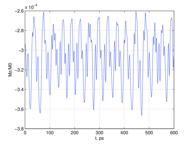
Figure 2: Oscillations of the longitudinal magnetization in the instability range at $K_{0}=7\times 10^{-3}$.

At $\Lambda=10^{3},\,\kappa=10^{-2},\,\eta_{0}=10^{2},\,h_{z}=-1$ the instability predicted by the linear theory must occur at $K_{0}=5\times 10^{-3}$ and disappear at $K_{0}=1\times 10^{-2}$. In our numerical experiments, increasing $K_{0}$ parameter from zero to the indicated threshold leads, in accordance with Eq. (56), to decrease of the damping of the magnetization vector precession about $z$ axis because of the negative damping caused by the STT mechanism. Incidentally, the absolute value of the (negative) $\hat{M}_{z}$ component decreases from $10^{-3}$ to $10^{-4}$ because of influence of the injection mechanism, that consists, also, with Eq. (54). Thus, the simulation results agree completely with the theory in the range below the instability threshold.

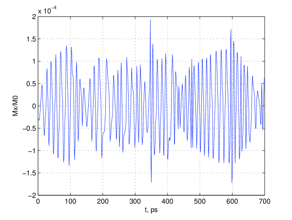
Figure 3: Beats of the transverse magnetization in the instability range at $K_{0}=8\times 10^{-3}$.

Of course, the instability range ($K_{0}>5\times 10^{-3}$), which is not described by the linear theory, is of more interest. At $K_{0}=5.1\times 10^{-3}$ undamped oscillations are observed. At $K_{0}=7\times 10^{-3}$ the precession oscillations of the transverse components $\hat{M}_{x},\,\hat{M}_{y}$ become almost sinusoidal with $\Delta T\approx 0.2$ period (this corresponds to angular frequency $\sim 3\times 10^{11}$ s^-1 at the chosen parameter values). The longitudinal component $\hat{M}_{z}$ oscillates periodically with a negative stationary background, however, the oscillation form is far from sinusoidal one (Fig. 2). At $K_{0}=8\times 10^{-3}$ the oscillations of $\hat{M}_{x},\,\hat{M}_{y}$ components take on a form of beats (Fig. 3), while they again become sinusoidal at $K_{0}=9\times 10^{-3}$. At $K_{0}=1\times 10^{-2}$ (this is the right boundary of the instability range in the linear theory) all the three components oscillate around zero values. Further, at $K_{0}=1.1\times 10^{-2}$ the oscillations hold yet, but at $K_{0}=1.2\times 10^{-2}$ they disappear almost completely, and they are absent at $K_{0}=1.5\times 10^{-2}$.

The subsequent increasing of the current leads only to rising magnetization in the positive direction due to the injection mechanism. At $K_{0}=2\Lambda/\eta_{0}$, the longitudinal component $\hat{M}_{z}$ reaches the maximal possible value $\hat{M}_{z}=2$ (the sublattices are flipped to a parallel position), then the (dimensionless) angular frequency is equal to $2\Lambda$ (this corresponds to $\sim 10^{13}$ s^-1). Such a situation corresponds to rather high current density, it is estimated as $2\times 10^{8}$ A/cm² at the above-mentioned parameter values.

9 Conclusions

The obtained results show a principal possibility of controlling frequency and damping of AFM resonance in FM/AFM junctions by means of spin-polarized current. Under low AFM magnetization induced by an external magnetic field perpendicular to the antiferromagnetism vector, the threshold current density corresponding to occurring instability is less substantially than in the FM–FM case. Near the threshold, the AFM resonance frequency increases, while damping decreases, that opens a possibility of generating oscillations in THz range.

Numerical simulation allows to trace behavior of the FM/AFM junction in the whole current density range. The instability range predicted by the linearized theory is broadened only slightly because of nonlinear effects. In the instability range undamped oscillation of sinusoidal or more complicated form including beats.

Under magnetic fields low compared to the exchange field, the induced magnetization is small in comparison with the sublattice magnetization, so that the stationary oscillation amplitude beyond the instability threshold is low, too.

Thus, the following features may be expected in comparison with the similar effects in FM/FM junctions. First, the instability threshold is to be lower because of the lower magnetization. This is a favorable fact facilitating observations. Second, the oscillation intensity beyond the threshold also lowers as a square of the magnetization. This may make the effect difficult to observe. Nevertheless, studying the current-driven nonlinear oscillations in FM/AFM structure is of principal interest, because the current induced instability can occur at relatively low current density, $\sim 10^{5}$ A/cm².

The simulation results reveal an interesting possibility of a spin-flip transition without magnetic field under the action of a high-density spin-polarized current only. Such a current overcomes the exchange forces and aligns the sublattice moments in parallel. Under such conditions, applying a low alternating magnetic field can excite precession of the magnetization vector at the AFM resonance frequencies, which may be as high as $3\times 10^{13}$ s^-1 or more. Such a THz resonator might be useful to detect and measure signals in THz range.

References

• [1] J.C. Slonczewski. J. Magn. Magn. Mater. 159, L1 (1996).
• [2] L. Berger. Phys. Rev. B 54, 9353 (1996).
• [3] J.A. Katine, F.J. Albert, R.A. Buhrman, E.B. Myers, D.C. Ralph. Phys. Rev. Lett. 84, 3149 (2000).
• [4] M. Tsoi, A.J.M. Jansen, J. Bass, W.-C. Chiang, M. Seck, V. Tsoi, P. Wyder Phys. Rev. Lett. 80, 4281 (1998).
• [5] A. Yamaguchi, T. Ono, S. Nasu, K. Miyake, K. Mibu, T. Shinjo. Phys. Rev. Lett. 92, 077205 (2004).
• [6] J.C. Sankey, P.M. Braganca, A.G.F. Garcia I.N. Krivorotov, R.A. Buhrman, D.C. Ralph. Phys. Rev. Lett. 96, 227601 (2006).
• [7] M. Watanabe, J. Okabayashi, H. Toyao, T. Yamaguchi, J. Yoshino. Appl. Phys. Lett. 92, 082506 (2008).
• [8] Yu.V. Gulyaev, P.E. Zilberman, A.I. Krikunov, E.M. Epshtein. Techn. Phys. 52, 1169 (2007).
• [9] Yu.V. Gulyaev, P.E. Zilberman, A.I. Panas, E.M. Epshtein. J. Exp. Theor. Phys. 107, 1027 (2008).
• [10] Yu.V. Gulyaev, P.E. Zilberman, S.G. Chigarev, E.M. Epshtein. Techn. Phys. Lett. 37, 154 (2011).
• [11] Yu.V. Gulyaev, P.E. Zilberman, E.M. Epshtein. J. Commun. Technol. Electron. 56, 863 (2011).
• [12] V.K. Sankaranarayanan, S.M. Yoon, D.Y. Kim, C.O. Kim, C.G. Kim. J. Appl. Phys. 96, 7428 (2004).
• [13] A. S. Núñez, R. A. Duine, P. Haney, A.H. MacDonald. Phys. Rev. B 73, 214426 (2006).
• [14] Z. Wei, A. Sharma, A.S. Nunez, P.M. Haney, R.A. Duine, J.Bass, A.H. MacDonald, M. Tsoi. Phys. Rev. Lett. 98, 116603 (2007).
• [15] Z. Wei, A. Sharma, J. Bass, M. Tsoi. J. Appl. Phys. 105, 07D113 (2009).
• [16] J. Basset, Z. Wei, M. Tsoi. IEEE Trans. Magn. 46, 1770 (2010).
• [17] S. Urazhdin, N. Anthony. Phys. Rev. Lett. 99, 046602 (2007).
• [18] H.V. Gomonay, V.M. Loktev. Low Temp. Phys. 34, 198 (2008).
• [19] H.V. Gomonay, V.M. Loktev. Phys. Rev. B 81, 144127 (2010).
• [20] K.M.D. Hals, Y. Tserkovnyak, A. Brataas. Phys. Rev. Lett. 106, 107206 (2011).
• [21] A.C. Swaving, R.A. Duine. Phys. Rev. B 83, 054428 (2011).
• [22] A.I. Akhiezer, V.G. Baryakhtar, S.V. Peletminslii. Spin Waves, North-Holland Pub. Co., Amsterdam, 1968.
• [23] C. Heide, P.E. Zilberman, R.J. Elliott, Phys. Rev. B 63, 064424 (2001).
• [24] Yu.V. Gulyaev, P.E. Zilberman, E.M. Epshtein, R.J. Elliott, JETP Lett. 76, 155 (2002).
• [25] Yu.V. Gulyaev, P.E. Zilberman, A.I. Panas, E.M. Epshtein. Physics — Uspekhi 52, 335 (2009).
• [26] Yu.V. Gulyaev, P.E. Zilberman, E.M. Epshtein, R.J. Elliott. J. Exp. Theor. Phys. 100, 1005 (2005).
• [27] A.G. Gurevich, G.A. Melkov. Magnetizsation Oscillations and Waves, CRC Press, Boca Raton, FL, 1996.
• [28] V.E. Dmitrienko, E.N. Ovchinnikova, J. Kokubun, K. Ishida. JETP Lett. 92, 383 (2010).
• [29] J.M. Robinson, P. Erdös. Phys. Rev. B 6, 3337 (1972).