Geometry of the set of mixed quantum states: An apophatic approach

Abstract

The set of quantum states consists of density matrices of order $N$, which are hermitian, positive and normalized by the trace condition. We analyze the structure of this set in the framework of the Euclidean geometry naturally arising in the space of hermitian matrices. For $N=2$ this set is the Bloch ball, embedded in $\mathbbm{R}^{3}$. For $N\geq 3$ this set of dimensionality $N^{2}-1$ has a much richer structure. We study its properties and at first advocate an apophatic approach, which concentrates on characteristics not possessed by this set. We also apply more constructive techniques and analyze two dimensional cross-sections and projections of the set of quantum states. They are dual to each other. At the end we make some remarks on certain dimension dependent properties.

Dedicated to prof. Bogdan Mielnik on the occasion of his 75-th birthday

I Introduction

Quantum information processing differs significantly from processing of classical information. This is due to the fact that the space of all states allowed in the quantum theory is much richer than the space of classical states Mi68 ; ACH93 ; MW98 ; AS03 ; GKM05 ; BZ06 . Thus an author of a quantum algorithm, writing a screenplay designed specially for the quantum scene, can rely on states and transformations not admitted by the classical theory.

For instance, in the theory of classical information the standard operation of inversion of a bit, called the NOT gate, cannot be represented as a concatenation of two identical operations on a bit. But the quantum theory allows one to construct the gate called $\sqrt{\rm NOT}$, which performed twice is equivalent to the flip of a qubit.

This simple example can be explained by comparing the geometries of classical and quantum state spaces. Consider a system containing $N$ perfectly distinguishable states. In the classical case the set of classical states, equivalent to $N$–point probability distributions, forms a regular simplex $\Delta_{N-1}$ in $N-1$ dimensions. Hence the set of pure classical states consists of $N$ isolated points. In a quantum set-up the set of states ${\cal Q}_{N}$, consisting of hermitian, positive and normalized density matrices, has $N^{2}-1$ real dimensions. Furthermore, the set of pure quantum states is connected, and for any two pure states there exist transformations that take us along a continuous path joining the two quantum pure states. This fact is one of the key differences between the classical and the quantum theories Ha01 .

The main goal of the present work is to provide an easy-to-read description of similarities and differences between the sets of classical and quantum states. Already when $N=3$ the geometric structure of the eight dimensional set ${\cal Q}_{3}$ is not easy to analyse nor to describe Bl76 ; AMM97 . Therefore we are going to use an apophatic approach, in which one tries to describe the properties of a given object by specifying simple features it does not have. Then we use a more conventional JS01 ; VDM02 ; Sollid constructive approach and investigate two-dimensional cross-sections and projections of the set ${\cal Q}_{3}$ Weis_tc ; Weis_cs ; Dunkl . Thereby a cross-section is defined as the intersection of a given set with an affine space. We happily recommend a very recent work for a more exhaustive discussion of the cross-sections Goyal .

II Classical and quantum states

A classical state is a probability vector $\vec{p}=(p_{1},p_{2},\dots,p_{N})$, such that $\sum_{i}p_{i}=1$ and $p_{i}\geq 0$ for $i=1,\dots N$. Assuming that a pure quantum state $|\psi\rangle$ belongs to an $N$–dimensional Hilbert space ${\cal H}_{N}$, a general quantum state is a density matrix $\rho$ of size $N$, which is hermitian, $\rho=\rho^{\dagger}$, with positive eigenvalues, $\rho\geq 0$, and normalized, Tr$\rho=1$. Note that any density matrix can be diagonalised, and then it has a probability vector along its diagonal. But clearly the space of all quantum states ${\cal Q}_{N}$ is significantly larger than the space of all classical states—there are $N-1$ free parameters in the probability vector, but there are $N^{2}-1$ free parameters in the density matrix.

The space of states, classical or quantum, is always a convex set. By definition a convex set is a subset of Euclidean space, such that given any two points in the subset the line segment between the two points also belongs to that subset. The points in the interior of the line segment are said to be mixtures of the original points. Points that cannot be written as mixtures of two distinct points are called extremal or pure. Taking all mixtures of three pure points we get a triangle $\Delta_{2}$, mixtures of four pure points form a tetrahedron $\Delta_{3}$, etc.

The individuality of a convex set is expressed on its boundary. Each point on the boundary belongs to a face, which is in itself a convex subset. To qualify as a face this convex subset must also be such that for all possible ways of decomposing any of its points into pure states, these pure states themselves belong to the subset. We will see that the boundary of ${\cal Q}_{N}$ is quite different from the boundary of the set of classical states.

II.1 Classical case: the probability simplex

The simplest convex body one can think of is a simplex $\Delta_{N-1}$ with $N$ pure states at its corners. The set of all classical states forms such a simplex, with the probabilities $p_{i}$ telling us how much of the $i$th pure state that has been mixed in. The simplex is the only convex set which is such that a given point can be written as a mixture of pure states in one and only one way.

The number $r$ of non–zero components of the vector $\vec{p}$ is called the rank of the state. A state of rank one is pure and corresponds to a corner of the simplex. Any point inside the simplex $\Delta_{N-1}$ has full rank, $r=N$. The boundary of the set of classical states is formed by states with rank smaller than $N$. Each face is itself a simplex $\Delta_{r-1}$. Corners and edges are special cases of faces. A face of dimension one less than that of the set itself is called a facet.

It is natural to think of the simplex as a regular simplex, with all its edges having length one. This can always be achieved, by defining the distance between two probability vectors $\vec{p}$ and $\vec{q}$ as

$$D[\vec{p},\vec{q}]=\sqrt{\frac{1}{2}\sum_{i=1}^{N}(p_{i}-q_{i})^{2}}\ .$$ (1)

The geometry is that of Euclid. With this geometry in place we can ask for the outsphere, the smallest sphere that surrounds the simplex, and the insphere, the largest sphere inscribed in it. Let the radius of the outsphere be $R_{N}$ and that of the insphere be $r_{N}$. One finds that $R_{N}/r_{N}=N-1$.

II.2 The Bloch ball

Another simple example of a convex set is a three dimensional ball. The pure states sit on its surface, and each such point is a zero dimensional face. There are no higher dimensional faces (unless we count the entire ball as a face). Given a point that is not pure it is now possible to decompose it in infinitely many ways as a mixture of pure states.

Remarkably this ball is the space of states ${\cal Q}_{2}$ of a single qubit, the simplest quantum mechanical state space. For concreteness introduce the Pauli matrices $\sigma_{1}={0\,1\choose 1\,0}$, $\sigma_{2}={0\,-{\rm i}\choose{\rm i}\,\,\,0}$, $\sigma_{3}={1\,\,\,0\choose 0\,-1}$. These three matrices form an orthonormal basis for the set of traceless Hermitian matrices of size two, or in other words for the Lie algebra of $SU(2)$. If we add the identity matrix $\sigma_{0}={\mathbbm{1}}={1\,0\choose 0\,1}$, we can expand an arbitrary state $\rho$ in this basis as

$$\rho=\frac{1}{2}{\mathbbm{1}}+\sum_{i=1}^{3}{\tau}_{i}{\sigma}_{i}\ ,$$ (2)

where the expansion coefficients are $\tau_{i}={\rm Tr}\rho\sigma_{i}/2$. These three numbers are real since the matrix $\rho$ is Hermitian. The three dimensional vector ${\vec{\tau}}=(\tau_{1},\tau_{2},\tau_{3})$ is called the Bloch vector (or coherence vector). If $\vec{\tau}=0$ we have the maximally mixed state. Pure states are represented by projectors, $\rho=\rho^{2}$.

Figure 1: The set of mixed states of a qubit forms the Bloch ball with pure states at the boundary and the maximally mixed state $\rho_{*}=\frac{1}{2}{\mathbbm{1}}$ at its center: The Hilbert–Schmidt distance between any two states is the length of the difference between their Bloch vectors, $||\vec{\tau}_{a}-\vec{\tau}_{b}||$.

Since the Pauli matrices are traceless the coefficient $\frac{1}{2}$ standing in front of the identity matrix assures that Tr$\rho=1$, but we must also ensure that all eigenvalues are non-negative. By computing the determinant we find that this is so if and only if the length of the Bloch vector is bounded, $||\vec{\tau}||^{2}\leq 1$. Hence ${\cal Q}_{2}$ is indeed a solid ball, with the pure states forming its surface—the Bloch sphere.

A simple but important point is that the set of classical states $\Delta_{1}$, which is just a line segment in this case, sits inside the Bloch ball as one of its diameters. This goes for any diameter, since we are free to regard any two commuting projectors as our classical bit. Two commuting projectors sit at antipodal points on the Bloch sphere. To ensure that the distance between any pair of antipodal equals one we define the distance between two density matrices $\rho_{A}$ and $\rho_{B}$ to be

$$D_{\rm HS}(\rho_{A},\rho_{B})\ =\ \sqrt{\frac{1}{2}\mbox{Tr}[(\rho_{A}-\rho_{B})^{2}]}\ .$$ (3)

This is known as the Hilbert-Schmidt distance. Let us express this in the Cartesian coordinate system provided by the Bloch vector,

$$D_{\rm HS}[\rho_{A},\rho_{B}]\ =\ \sqrt{\sum_{i=1}^{3}(\tau^{A}_{i}-\tau^{B}_{i})^{2}}\ =\ ||\vec{\tau}^{A}-\vec{\tau}^{B}||\ .$$ (4)

This is the Euclidean notion of distance.

II.3 Quantum case: ${\cal Q}_{N}$

When $N>2$ the quantum state space is no longer a solid ball. It is always a convex set however. Given two density matrices, that is to say two positive hermitian matrices $\rho,\sigma\in{\cal Q}_{N}$. It is then easy to see that any convex combination of these two states, $a\rho+(1-a)\sigma\in{\cal Q}_{N}$ where $a\in[0,1]$, must be a positive matrix too, and hence it belongs to ${\cal Q}_{N}$. This shows that the set of quantum states is convex. For all $N$ the face structure of the boundary can be discussed in a unified way. Moreover it remains true that ${\cal Q}_{N}$ is swept out by rotating a classical probability simplex $\Delta_{N-1}$ in $\mathbbm{R}^{N^{2}-1}$, but for $N>2$ there are restrictions on the allowed rotations.

To make these properties explicit we start with the observation that any density matrix can be represented as a convex combination of pure states

$$\rho=\sum_{i=1}^{k}p_{i}\,|\phi_{i}\rangle\langle\phi_{i}|,$$ (5)

where $\vec{p}=(p_{1},p_{2},\dots,p_{k})$ is a probability vector. In contrast to the classical case there exist infinitely many decompositions of any mixed state $\rho\neq\rho^{2}$. The number $k$ can be arbitrarily large, and many different choices can be made for the pure states $|\phi_{i}\rangle$. But there does exist a distinguished decomposition. Diagonalising the density matrix we find its eigenvalues $\lambda_{i}\geq 0$ and eigenvectors $|\psi_{i}\rangle$. This allows us to write the eigendecomposition of a state,

$$\rho=\sum_{j=1}^{N}\lambda_{j}|\psi_{j}\rangle\langle\psi_{j}|\ .$$ (6)

The number $r$ of non-zero components of the probability vector $\vec{\lambda}$ is called the rank of the state $\rho$, and does not exceed $N$. This is the usual definition of the rank of a matrix, and by happy accident it agrees with the definition of rank in convex set theory: the rank of a point in a convex set is the smallest number of pure points needed to form the given point as a mixture.

Consider now a general convex set in $d$ dimensions. Any point belonging to it can be represented by a convex combination of not more than $d+1$ extremal states. Interestingly, ${\cal Q}_{N}$ has a peculiar geometric structure since any given density operator $\rho$ can be represented by a combination of not more than $N$ pure states, which is much smaller than $d+1=N^{2}$. In Hilbert space these $N$ pure states are the orthogonal eigenvectors of $\rho$. If we adopt the Hilbert-Schmidt definition of distance (3) they form a copy of the classical state space, the regular simplex $\Delta_{N-1}$.

Conversely, every density matrix can be reached from a diagonal density matrix by means of an $SU(N)$ transformation. Such transformations form a subgroup of the rotation group $SO(N^{2}-1)$. Therefore any density matrix can be obtained by rotating a classical probability simplex around the maximally mixed state, which is left invariant by rotations. However, when $N>2$ $SU(N)$ is a proper subgroup of $SO(N^{2}-1)$, which is why ${\cal Q}_{N}$ forms a solid ball only if $N=2$. The relative sizes of the outsphere and the insphere are still related by $R_{N}/r_{N}=N-1$.

Figure 2: The set ${\cal Q}_{3}$ of quantum states of a qutrit contains positive semi-definite matrices with spectrum from the simplex $\Delta_{2}$ of classical states. The corners of the triangle become the $4D$ set of pure states, the edges lead to the $7D$ boundary $\partial{\cal Q}_{3}$, while interior of the triangle gives the interior of the $8D$ convex body. The set ${\cal Q}_{3}$ is inscribed inside a $7$–sphere of radius $R_{3}=\sqrt{2/3}$ and it contains an $8$–ball of radius $r_{3}=1/\sqrt{6}$.

The boundary of the set ${\cal Q}_{N}$ shows some similarities with that of its classical cousin. It consists of all matrices whose rank is smaller than $N$. There will be faces of rank 1 (the pure states), of rank 2 (in themselves they are copies of ${\cal Q}_{2}$), and so on up to faces of rank $N-1$ (copies of ${\cal Q}_{N-1}$). Note that there are no hard edges: the minimal non-extremal faces are solid three dimensional balls. The largest faces have a dimension much smaller than the dimension of the boundary of ${\cal Q}_{N}$. As in the classical case, any face can be described as the intersection of the convex set with a bounding hyperplane in the container space. In technical language one says that all faces are exposed. Note also that every point on the boundary belongs to a face that is tangent to the insphere. This has the interesting consequence that the area $A$ of the boundary is related to the volume $V$ of the body by

$$\frac{rA}{V}=d\ ,$$ (7)

where $r$ is the radius of the insphere and $d$ is the dimension of the body (in this case $d=N^{2}-1$) SBZ06 . Incidentally the volume of ${\cal Q}_{N}$ is known explicitly ZS03 .

There are differences too. A typical state on the boundary has rank $N-1$, and any two such states can be connected with a curve of states such that all states on the curve have the same rank. In this sense ${\cal Q}_{N}$ is more like an egg than a polytope Marmo .

We can regard the set of $N$ by $N$ matrices as a vector space (called Hilbert-Schmidt space), endowed with the scalar product

$$\langle A|B\rangle_{\rm HS}=\frac{1}{2}{\rm Tr}A^{\dagger}B\ .$$ (8)

The set of hermitian matrices with unit trace is not a vector space as it stands, but it can be made into one by separating out the traceless part. Thus we can represent a density matrix as

$$\rho=\frac{1}{N}{\mathbbm{1}}+u\ ,$$ (9)

where $u$ is traceless. The set of traceless matrices is an Euclidean subspace of Hilbert-Schmidt space, and the Hilbert-Schmidt distance (3) arises from this scalar product. In close analogy to eq. (2) we can introduce a basis for the set of traceless matrices, and write the density matrix in the generalized Bloch vector representation,

$$\rho=\frac{1}{N}{\mathbbm{1}}+\sum_{i=1}^{N^{2}-1}u_{i}{\gamma}_{i}\ .$$ (10)

Here $\gamma_{i}$ are hermitian basis vectors. The components $u_{i}$ must be chosen such that $\rho$ is a positive definite matrix.

II.4 Dual and self-dual convex sets

Both the classical and the quantum state spaces have the remarkable property that they are self-dual. But the word duality has many meanings. In projective geometry the dual of a point is a plane. If the point is represented by a vector ${\vec{x}}$, we can define the dual plane as the set of vectors ${\vec{y}}$ such that

$${\vec{x}}\cdot{\vec{y}}=-1\ .$$ (11)

The dual of a line is the intersection of a one-parameter family of planes dual to the points on the line. This is in itself a line. The dual of a plane is a point, while the dual of a curved surface is another curved surface—the envelope of the planes that are dual to the points on the original surface. To define the dual of a convex body with a given boundary we change the definition slightly, and include all points on one side of the dual planes in the dual. Thus the dual $X^{*}$ of a convex body $X$ is defined to be

$$X^{*}=\{{\vec{x}}\mid 1+{\vec{x}}\cdot{\vec{y}}\;\geq\;0\ \forall{\vec{y}}\in X\}\ .$$ (12)

The dual of a convex body including the origin is the intersection of half-spaces $\{{\vec{x}}\mid 1+{\vec{x}}\cdot{\vec{y}}\geq 0\}$ for extremal points ${\vec{y}}$ of $X$ R70 . If we enlarge a convex body the conditions on the dual become more stringent, and hence the dual shrinks. The dual of a sphere centred at the origin is again a sphere, so a sphere (of suitable radius) is self-dual. The dual of a cube is an octahedron. The dual of a regular tetrahedron is another copy of the original tetrahedron, possibly of a different size. Hence this is a self-dual body. Convex subsets $F\subset X$ are mapped to subsets of $X^{*}$ by

$$F\;\mapsto\;\widehat{F}:=\{{\vec{x}}\in X^{*}\mid 1+{\vec{x}}\cdot{\vec{y}}=0\,\forall{\vec{y}}\in F\}\ .$$ (13)

Geometrically, $\widehat{F}$ equals $X^{*}$ intersected with the dual affine space (11) of the affine span of $F$. If the origin lies in the interior of the convex body $X$ then $F\mapsto\widehat{F}$ is a one-to-one inclusion-reversing correspondence between the exposed faces of $X$ and of $X^{*}$ Gr03 . If $X$ is a tetrahedron, then vertices and faces are exchanged, while edges go to edges.

What we need in order to prove the self-duality of ${\cal Q}_{N}$ is the key fact that a hermitian and unit trace matrix $\sigma$ is a density matrix if and only if

$${\rm Tr}\sigma\rho\ \geq\ 0$$ (14)

for all density matrices $\rho$. It will be convenient to think of a density matrix $\rho$ as represented by a “vector” $u$, as in eq. (9). As a direct consequence of eq. (14) the set of quantum states ${\cal Q}_{N}$ is self-dual in the precise sense that

$${\cal Q}_{N}-{\rm 1\mskip-4.0mul}/N=\{u\mid 1/N+{\rm Tr}(uv)\geq 0\,\forall v\in{\cal Q}_{N}-{\rm 1\mskip-4.0mul}/N\}.$$ (15)

In this equation the trace is to be interpreted as a scalar product in a vector space. Duality (13) exchanges faces of rank $r$ (copies of ${\cal Q}_{r}$) and faces of rank $N-r$ (copies of ${\cal Q}_{N-r}$).

Self-duality is a key property of state spaces Wilce ; Ududec , and we will use it extensively when we discuss projections and cross-sections of ${\cal Q}_{N}$. This notion is often introduced in the larger vector space consisting of all hermitian matrices, with the origin at the zero matrix. The set of positive semi-definite matrices forms a cone in this space, with its apex at the origin. It is a cone because any positive semi-definite matrix remains positive semi-definite if multiplied by a positive real number. This defines the rays of the cone, and each ray intersects the set of unit trace matrices exactly once. The dual of this cone is the set of all matrices $a$ such that Tr$ab\geq 0$ for all matrices $b$ within the cone—and indeed the dual cone is equal to the original, so it is self-dual.

III An apophatic approach to the qutrit

For $N=3$ we are dealing with the states of the qutrit. The Gell-Mann matrices are a standard choice Goyal for the eight matrices $\gamma_{i}$, and the expansion coefficients are $\tau_{i}=\frac{1}{2}{\rm Tr}\rho\gamma_{i}$. Unfortunately, although the sufficient conditions for $\vec{\tau}$ to represent a state are known AMM97 ; Ki03 ; KK05 , they do not improve much our understanding of the geometry of ${\cal Q}_{3}$.

We know that the set of pure states has 4 real dimensions, and that the faces of ${\cal Q}_{3}$ are copies of the 3D Bloch ball, filling out the 7 dimensional boundary. The centres of these balls touch the largest inscribed sphere of ${\cal Q}_{3}$. But what does it all really look like?

We try to answer this question by presenting some 3D objects, and explaining why they cannot serve as models of ${\cal Q}_{3}$. Apart from the fact that our objects are not eight dimensional, all of them lack some other features of the set of quantum states.

Fig. 3 presents a hairy set which is nice but not convex. Fig. 4 shows a ball, and we know that ${\cal Q}_{3}$ is not a ball. It is not a polytope either, so the polytope shown in Fig. 5 cannot model the set of quantum states.

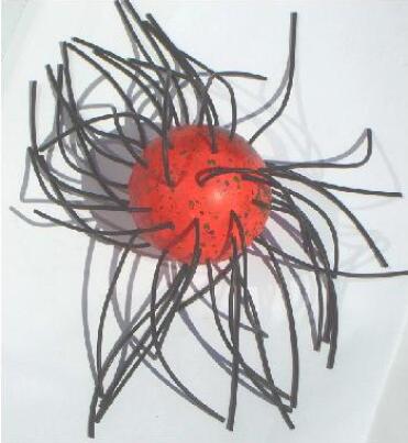
Figure 3: Apophatic approach: this object is not a good model of the set ${\cal Q}_{3}$ as it is not a convex set.

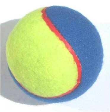
Figure 4: The set ${\cal Q}_{3}$ is not a ball…

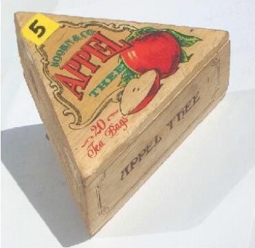
Figure 5: The set ${\cal Q}_{3}$ is not a polytope…

Let us have a look at the cylinder shown in Fig. 6, and locate the extremal points of the convex body shown. This subset consists of the two circles surrounding both bases. This is a disconnected set, in contrast to the connected set of pure quantum states. However, if one splits the cylinder into two halves and rotates one half by $\pi/2$ as shown in Fig. 7, one obtains a body with a connected set of pure states. A similar model can be obtained by taking the convex hull of the seam of a tennis ball: the one dimensional seam contains the extremal points of this set and forms a connected set.

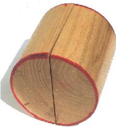
Figure 6: The set of pure states in ${\cal Q}_{3}$ is connected, but for the cylinder the pure states form two circles.

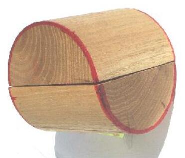
Figure 7: This is now the convex hull of a single space curve, but one cannot inscribe copies of the classical set $\Delta_{2}$ in it.

Thus the seam of the tennis ball (look again at Fig. 4) corresponds to the $4D$ connected set of pure states of $N=3$ quantum system. The convex hull of the seam forms a $3D$ object which is easy to visualize, and serves as our first rough model of the solid $8D$ body ${\cal Q}_{3}$ of qutrit states. However, a characteristic feature of the latter is that each one of its points belongs to a cross-section which is an equilateral triangle $\Delta_{2}$. (This is the eigenvector decomposition.) The convex set determined by the seam of the tennis ball, and the set shown in Fig. 7, do not have this property.

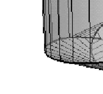
Figure 8: a) The space curve ${\vec{x}}(t)$ modelling pure quantum states is obtained by rotating an equilateral triangle according to Eq. (16) —three positions of the triangle are shown); b) The convex hull $C$ of the curve models the set of all quantum states.

As we have seen ${\cal Q}_{3}$ can be obtained if we take an equilateral triangle $\Delta_{2}$ and subject it to $SU(3)$ rotations in eight dimensions. We can try to do something similar in three dimensions. If we rotate a triangle along one of its bisections we obtain a cone, for which the set of extremal states consists of a circle and an apex (see Fig. 10 b)), a disconnected set. We obtain a better model if we consider the space curve

$${\vec{x}}(t)\;=\;\bigl{(}\cos(t)\cos(3t),\ \cos(t)\sin(3t),\ -\sin(t)\bigr{)}^{\rm T}\;.$$ (16)

Note that the curve is closed, ${\vec{x}}(t)={\vec{x}}(t+2\pi)$, and belongs to the unit sphere, $||{\vec{x}}(t)||=1$. Moreover

$$||{\vec{x}}(t)-{\vec{x}}(t+\tfrac{1}{3}2\pi)||=\sqrt{3}$$ (17)

for every value of $t$. Hence every point ${\vec{x}}(t)$ belongs to an equilateral triangle with vertices at

$${\vec{x}}(t),\qquad{\vec{x}}(t+\tfrac{1}{3}2\pi),\qquad\text{and}\qquad{\vec{x}}(t+\tfrac{2}{3}2\pi)\ .$$

They span a plane including the $z$-axis for all times $t$. During the time $\Delta t=\tfrac{2\pi}{3}$ this plane makes a full turn about the $z$-axis, while the triangle rotates by the angle $2\pi/3$ within the plane—so the triangle has returned to a congruent position. The curve ${\vec{x}}(t)$ is shown in Fig. 8 a) together with exemplary positions of the rotating triangle, and Fig. 8 b) shows its convex hull $C$. This convex hull is symmetric under reflections in the $(x$-$y)$ and $(x$-$z)$ planes. Since the set of pure states is connected this is our best model so far of the set of quantum pure states, although the likeness is not perfect.

It is interesting to think a bit more about the boundary of $C$. There are three flat faces, two triangular ones and one rectangular. The remaining part of the boundary consists of ruled surfaces: they are curved, but contain one dimensional faces (straight lines). The boundary of the set shown in Fig. 7 has similar properties. The ruled surfaces of $C$ have an analogue in the boundary of the set of quantum states ${\cal Q}_{3}$, we have already noted that a generic point in the boundary of ${\cal Q}_{3}$ belongs to a copy of ${\cal Q}_{2}$ (the Bloch ball), arising as the intersection of ${\cal Q}_{3}$ with a hyperplane. The flat pieces of $C$ have no analogues in the boundary of ${\cal Q}_{3}$, apart from Bloch balls (rank two) and pure states (rank one) no other faces exist.

Still this model is not perfect: Its set of pure states has self-intersections. Although it is created by rotating a triangle, the triangles are not cross-sections of $C$. It is not true that every point on the boundary belongs to a face that touches the largest inscribed sphere, as it happens for the set of quantum states SBZ06 . Indeed its boundary is not quite what we want it to be, in particular it has non-exposed faces—a point to which we will return. Above all this is not a self-dual body.

IV A constructive approach

The properties of the eight-dimensional convex set ${\cal Q}_{3}$ might conflict if we try to realize them in dimension three. Instead of looking for an ideal three dimensional model we shall thus use a complementary approach. To reduce the dimensionality of the problem we investigate cross-sections of the $8D$ set ${\cal Q}_{3}$ with a plane of dimension two or three, as well as its orthogonal projections on these planes—the shadows cast by the body on the planes, when illuminated by a very distant light source. Clearly the cross-sections will always be contained in the projections, but in exceptional cases they may coincide.

What kind of cross-sections arise? In the classical case it is known that every convex polytope arises as a cross-section of a simplex $\Delta_{N-1}$ of sufficiently high dimension Gr03 . It is also true that every convex polytope arises as the projection of a simplex. But what are the cross-sections and the projections of ${\cal Q}_{N}$? There has been considerable progress on this question recently. The convex set is said to be a spectrahedron if it is a cross-section of a cone of semi-positive definite matrices of some given size. In the branch of mathematics known as convex algebraic geometry one asks what kind of convex bodies that can be obtained as projections of spectrahedra. Surprisingly, the convex hull of any trigonometric space curve in three dimensions can be so obtained Henrion . This includes our set $C$, which can be shown to be a projection of an $8$-dimensional cross-section of the $35D$ set ${\cal Q}_{6}$ of quantum states of size $N=6$. We do so in Appendix A.

IV.1 The duality between projections and cross-sections

In the vector space of traceless hermitian matrices we choose a linear subspace $U$. The intersection of the convex body ${\cal Q}_{N}$ of quantum states with the subspace $U+{\rm 1\mskip-4.0mul}/N$ through the maximally mixed state ${\rm 1\mskip-4.0mul}/N$ is the cross-section $S_{U}$, and the orthogonal projection of ${\cal Q}_{N}$ down to $U$ is the projection $P_{U}$. There exists a beautiful relation between projections and cross-sections, holding for self-dual convex bodies such as the classical and the quantum state spaces Weis_cs . For them cross-sections and projections are dual to each other, in the sense that

$$S_{U}-{\rm 1\mskip-4.0mul}/N=\{u\mid 1/N+{\rm Tr}(uv)\geq 0\ \forall v\in P_{U}\}\ \$$ (18)

and

$$P_{U}=\{u\mid 1/N+{\rm Tr}(uv)\geq 0\ \forall v\in S_{U}-{\rm 1\mskip-4.0mul}/N\}\ .$$ (19)

This is best explained in a picture (namely Fig. 9). A special case of these dualities is the self-duality of the full state-space, eq. (15).

Figure 9: The triangle is self-dual. We intersect it with a one-dimensional subspace through the centre, $U$, and obtain a cross-section extending from $a$ to $b$. The dual of this line in the plane is a 2-dimensional strip, and when we project this onto $U$ we obtain a projection extending from $A$ to $B$, which is dual to the cross-section within $U$.

Let us look at two examples for ${\cal Q}_{3}$, choosing the vector space $U$ to be three dimensional. In Fig.10 a) we show the cross-section containing all states of the form

$$\rho=\left(\begin{array}[]{ccc}1/3&x&y\\ x&1/3&z\\ y&z&1/3\end{array}\right)\ ,\hskip 14.22636pt\rho\geq 0\ .$$ (20)

They form an overfilled tetrapak cartoon Bl76 , also known as an elliptope Sturmfels and an obese tetrahedron Goyal . Like the tetrahedron it has six straight edges. Its boundary is known as Cayley’s cubic surface, and it is smooth everywhere except at the four vertices. In the picture it is surrounded by its dual projection, which is the convex hull of a quartic surface known as Steiner’s Roman surface. To understand the shape of the dual, start with a pair of dual tetrahedra (one of them larger than the other). Then we “inflate” the small tetrahedron a little, so that its facets turn into curved surfaces. It grows larger, so its dual must shrink—the vertices of the dual become smooth, while the facets of the dual will be contained within the original triangles. What we see in Fig.10 a) is a “critical” case, in which the facets of the dual have shrunk to four circular disks that just touch each other in six special points.

In Fig.10 b) we see the cross-section containing all states (positive matrices) of the form

$$\rho=\left(\begin{array}[]{ccc}1/3+z/\sqrt{3}&x-{\rm i}y&0\\ x+{\rm i}y&1/3+z/\sqrt{3}&0\\ 0&0&1/3-2z/\sqrt{3}\end{array}\right)\ .$$ (21)

This cross-section is a self-dual set, meaning that the projection to this 3-dimensional plane coincides with the cross-section. In itself it is the state space of a real subalgebra of the qutrit obervables. There exist also two-dimensional self-dual cross-sections, which are simply copies of the classical simplex $\Delta_{2}$—the state space of the subalgebra of diagonal matrices.

Figure 10: a) The cross-section $S_{U}-{\rm 1\mskip-4.0mul}/3$ defined in (20) of the qutrit quantum states ${\cal Q}_{3}$ is drawn inside the projection $P_{U}$ of ${\cal Q}_{3}$. b) The cone is self-dual, it is a cross-section and a projection of ${\cal Q}_{3}$ with $S_{U}-{\rm 1\mskip-4.0mul}/3=P_{U}$.

IV.2 Two-dimensional projections and cross-sections

To appreciate what we see in cross-sections and projections we will concentrate on 2-dimensional screens.

We can compute 2D projections using the fact that they are dual to a cross-section. But we can also use the notion of the numerical range $W$ of a given operator $A$, a subset of the complex plane HJ2 ; GR97 ; GPMSZ10

$$W(A)=\{z\in{\mathbbm{C}}:z={\rm Tr}\rho A,\ \rho\in{\cal Q}_{N}\}\ .$$ (22)

If the matrix $A$ is hermitian its numerical range reduces to a line segment, otherwise it is a convex region of the complex plane. To see the connection to projections, observe that changing the trace of $A$ gives rise to a translation of the whole set, so we may as well fix the trace to equal unity. Then we can write for some $\lambda\in{\mathbb{C}}$

$$A=\lambda{\mathbbm{1}}+u+{\rm i}v\ ,$$ (23)

where $u$ and $v$ are traceless hermitian matrices. It follows that the set of all possible numerical ranges $W(A)$ of arbitrary matrices $A$ of order $N$ is affinely equivalent to the set of orthogonal projections of ${\cal Q}_{N}$ on a $2$-plane Dunkl ; Henrionrange . Thus to understand the structure of projections of ${\cal Q}_{N}$ onto a plane it is sufficient to analyze the geometry of numerical ranges of any operator of size $N$. For instance, in the simplest case of a matrix $A$ of order $N=2$, its numerical range forms an elliptical disk, which may reduce to an interval. These are just possible (not necessarily orthogonal) projections of the Bloch ball ${\cal Q}_{2}$ onto a plane.

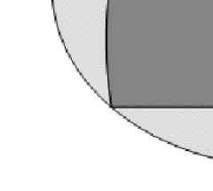
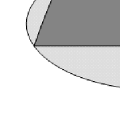
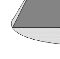
Figure 11: The drawings are dual pairs of planar cross-sections $S_{U}-{\rm 1\mskip-4.0mul}/3$ (dark) and projections $P_{U}$ (bright) of the convex body of qutrit quantum states ${\cal Q}_{3}$. Drawing a is obtained from the 3D dual pair in Fig. 10 a) and b)–d) are derived from the self-dual cone in Fig. 10 b). The cross-sections in b)–d) have an elliptic, parabolic and hyperbolic boundary piece, respectively.

In the case of a matrix $A$ of order $N=3$ the shape of its numerical range was characterized algebraically in K51 ; KRS97 . Regrouping this classification we divide the possible shapes into four cases according to the number of flat boundary parts: The set $W$ is compact and its boundary $\partial W$

1. has no flat parts. Then $W$ is strictly convex, it is bounded by an ellipse or equals the convex hull of a (irreducible) sextic space curve;

2. has one flat part, then $W$ is the convex hull of a quartic space curve – e.g. $W$ is the convex hull of a trigonometric curve known as the cardioid;

3. has two flat parts, then $W$ is the convex hull of an ellipse and a point outside it;

4. has three flat parts, then $W$ is a triangle with corners at eigenvalues of $A$.

In case 4 the matrix $A$ is normal, $AA^{\dagger}=A^{\dagger}A$, and the numerical range is a projection of the simplex $\Delta_{2}$ onto a plane. Looking at the planar projections of ${\cal Q}_{3}$ shown in Fig.11 we recognize cases 2 and 3. All four cases are obtained as projections of the Roman surface in Fig. 10 a) or the cone shown in Fig. 10 b). A rotund shape and one with two flats are obtained as a projection of both 3D bodies. A triangle is obtained from the cone and a shape with one flat from the Roman surface.

In order to actually calculate a $2D$ projection $P:=\{({\rm Tr}u\rho,{\rm Tr}v\rho)^{\rm T}\in\mathbb{R}^{2}\mid\rho\in{\cal Q}_{3}\}$ of the set ${\cal Q}_{3}$ determined by two traceless hermitian matrices $u$ and $v$ one may proceed as follows HJ2 . For every non-zero matrix $F$ in the real span of $u$ and $v$ we calculate the maximal eigenvalue $\lambda$ and the corresponding normalized eigenvector $|\psi\rangle$ with $F|\psi\rangle=\lambda|\psi\rangle$. Then $(\langle\psi|u|\psi\rangle,\langle\psi|v|\psi\rangle)^{\rm T}$ belongs to the projection $P$, and these points cover all exposed points of $P$.

IV.3 Exposed and non-exposed faces

Exemplary sets	disk $a)$	drop $b)$	truncated disk $c)$	truncated drop $d)$
non-exposed points $(*)$	no	yes	no	yes
non-polyhedral corners $(o)$	no	no	yes	yes
set is self-dual	yes	no	no	yes

Figure 12: Exemplary convex sets and their duals. Symbols: non-exposed point ($*$), polyhedral corners ($+$) and non-polyhedral corners $(o)$. Sets a) and d) are self-dual, while b) and c) is a dual pair. Sets a) and c) have properties like 2D cross-sections of ${\cal Q}_{N}$, while sets a) and b) could be obtained from ${\cal Q}_{N}$ by projection.

An exposed face of a convex set $X$ is the intersection of $X$ with an affine hyperplane $H$ such that $X\setminus H$ is convex, i.e. $H$ intersects $X$ only at the boundary. Examples in the plane are the boundary points of the disk in Fig. 12 a) or the boundary segments in panels b) and d). A non-exposed face of $X$ is a face of $X$ that is not an exposed face. In dimension two non-exposed faces are non-exposed points, they are the endpoints of boundary segment of $X$ which are not exposed faces by themselves. Examples are the lower endpoints of the boundary segments in Fig. 12 b) or d).

It is known that cross-sections of ${\cal Q}_{N}$ have no non-exposed faces. On the other hand the twisted cylinder (see Fig. 7) and the convex hull $C$ of the space curve (Fig. 8) do have non-exposed faces of dimension one. In contrast to cross-sections, projections of ${\cal Q}_{N}$ can have non-exposed points, see e.g. the planar projections of ${\cal Q}_{3}$ in Fig. 11. They are related to discontinuities in certain entropy functionals (in use as information measures) Knauf_Weis .

The dual concept to exposed face is normal cone Weis_tc . The normal cone of a two-dimensional convex set $X\subset\mathbb{R}^{2}$ at $(x_{1},x_{2})\in X$ is

$$\{(y_{1},y_{2})^{\rm T} \in{\mathbb{R}}^{2}\mid$$

$$(z_{1}-x_{1})y_{1}+(z_{2}-x_{2})y_{2}\leq 0\;\forall(z_{1},z_{2})\in X\}.$$

The normal cone generalizes outward pointing normal vectors of a smooth boundary curve of $X$ to points $(x_{1},x_{2})$ where this curve is not smooth. Then the dimension of the normal cone is two and we call $(x_{1},x_{2})$ a corner. The examples in Fig. 12 have $0,1,2,3$ corners from left to right. There are different types of corners: The top corners of Fig. 12 b) and d) are polyhedral, i.e. they are intersections of two boundary segments. If a corner is not the intersection of two boundary segments we call it non-polyhedral. The bottom corners of c) and d) are non-polyhedral corners. Polyhedral and non-polyhedral corners are characterized in Weis_dn in terms of normal cones. From this characterization it follows that any corner of a two-dimensional projection of ${\cal Q}_{N}$ is polyhedral Weis_tc . An analogue property holds in higher dimensions but it can not be formulated in terms of polyhedra. Fig. 11 shows that two-dimensional cross-sections of ${\cal Q}_{3}$ can have non-polyhedral corners.

Given a two-dimensional convex body including the origin in the interior, the duality (13) maps non-exposed points onto the set of non-polyhedral corners of the dual convex body. There will be one or two non-exposed points in each fiber depending on whether the corner does or does not lie on a boundary segment of the dual body Weis_dn . We conclude that a two-dimensional self-dual convex set has no non-exposed points if and only if all its corners are polyhedral.

V When the dimension matters

So far we have discussed the qutrit, and properties of the qutrit that generalise to any dimension $N$. But what is special about a quantum system whose Hilbert space has dimension $N$? The question gains some relevance from recent attempts to find direct experimental signatures of the dimension,

One obvious answer is that if and only if $N$ is a composite number, the system admits a description in terms of entangled subsystems. But we can look for an answer in other directions too. We emphasised that a regular simplex $\Delta_{N-1}$ can be inscribed in the quantum state space ${\cal Q}_{N}$. But in the Bloch ball we can clearly inscribe not only $\Delta_{1}$ (a line segment), but also $\Delta_{2}$ (a triangle) and $\Delta_{3}$ (a tetrahedron). If we insist that the vertices of the inscribed simplex should lie on the outsphere of ${\cal Q}_{N}$, and also that the simplex should be centred at the maximally mixed state, then this gives rise to a non-trivial problem once the dimension $N>2$. This is clear from our model of the latter as the convex hull of the seam of a tennis ball, or in other words because the set of pure states form a very small subset of the outsphere. Still we saw, in Fig. 10 a), that not only $\Delta_{2}$ but also $\Delta_{3}$ can be inscribed in ${\cal Q}_{3}$, and as a matter of fact so can $\Delta_{5}$ and $\Delta_{8}$. But is it always possible to inscribe the regular simplex $\Delta_{N^{2}-1}$ in ${\cal Q}_{N}$, in such a way that the $N^{2}$ vertices are pure states? Although the answer is not obvious, it is perhaps surprising to learn that the answer is not known, despite a considerable amount of work in recent years.

The inscribed regular simplices $\Delta_{N^{2}-1}$ are known as symmetric informationally complete positive operator valued measures, or SIC-POVMs for short. Their existence has been established, by explicit construction, in all dimensions $N\leq 16$ and in a handful of larger dimensions. The conjecture is that they always exist Scott . But the available constructions have so far not revealed any pattern allowing one to write down a solution for all dimensions $N$. Already here the quantum state space begins to show some $N$-dependent individuality.

Another question where the dimension matters concerns complementary bases in Hilbert space. As we have seen, given a basis in Hilbert space, there is an $(N-1)$-dimensional cross-section of ${\cal Q}_{N}$ in which these vectors appear as the vertices of a regular simplex $\Delta_{N-1}$. We can—for instance for tomographic reasons Wootters —decide to look for two such cross-sections placed in such a way that they are totally orthogonal with respect to the trace inner product. If the two cross-sections are spanned by two regular simplices stemming from two Hilbert space bases $\{|e_{i}\rangle\}_{i=0}^{N-1}$ and $\{|f_{i}\rangle\}_{i=0}^{N-1}$, then the requirement on the bases is that

$$|\langle e_{i}|f_{j}\rangle|^{2}=\frac{1}{N}$$ (24)

for all $i,j$. Such bases are said to be complementary, and form a key element in the Copenhagen interpretation of quantum mechanics Schwinger . But do they exist for all $N$?

The answer is yes. To see this, let one basis be the computational one, and let the other be expressed in terms of it as the column vectors of the Fourier matrix

$$F_{N}=\frac{1}{\sqrt{N}}\left[\begin{array}[]{ccccc}1&1&1&\dots&1\\ 1&\omega&\omega^{2}&\dots&\omega^{N}\\ 1&\omega^{2}&\omega^{4}&\dots&\omega^{2(N-1)}\\ \vdots&\vdots&\vdots&&\vdots\\ 1&\omega^{N-1}&\omega^{2(N-1)}&\dots&\omega^{(N-1)^{2}}\end{array}\right]\ ,$$ (25)

where $\omega=e^{2\pi i/N}$ is a primitive root of unity. The Fourier matrix is an example of a complex Hadamard matrix, a unitary matrix all of whose matrix elements have the same modulus.

We are interested in finding all possible complementary pairs up to unitary equivalences. The latter are largely fixed by requiring that one member of the pair is the computational basis, since the second member will then be defined by a complex Hadamard matrix. The remaining freedom is taken into account by declaring two complex Hadamard matrices $H$ and $H^{\prime}$ to be equivalent if they can be related by

$$H^{\prime}=D_{1}P_{1}HP_{2}D_{2}\ ,$$ (26)

where $D_{i}$ are diagonal unitary matrices and $P_{i}$ are permutation matrices.

The task of classifying pairs of cross-sections of ${\cal Q}_{N}$ forming simplices $\Delta_{N-1}$ and sitting in totally orthogonal $N$-planes is therefore equivalent to the problem of classifying complementary pairs of bases in Hilbert space. This problem in turn is equivalent to the problem of classifying complex Hadamard matrices of a given size. But the latter problem has been open since it was first raised by Sylvester and Hadamard, back in the nineteenth century. It has been completely solved only for $N\leq 5$, and it was recently almost completely solved for $N=6$ Szollosi .

More is known if we restrict ourselves to continuous families of complex Hadamard matrices that include the Fourier matrix. Then it has been known for some time TZ08 that the dimension of such a family is bounded from above by

$$d_{F_{N}}=\sum_{k=0}^{N-1}\mbox{gcd}(k,N)-(2N-1)\ ,$$ (27)

where gcd denotes the largest common divisor, and gcd$(0,N)=N$. We subtracted the $2N-1$ dimensions that arise trivially from eq. (26). Moreover, if $N=p^{k}$ is a power of prime number $p$ this bound is saturated by families that have been constructed explicitly. In particular, if $N$ is a prime number $d_{F_{p}}=0$, and the Fourier matrix is an isolated solution. For $N=4$ on the other hand there exists a one-parameter family of inequivalent complex Hadamard matrices.

Further results on this question were presented in Białowieża Nuno . In particular the above bound is not achieved for any $N$ not equal to a prime power and not equal to 6. It turns out that the answer depends critically on the nature of the prime number decomposition of $N$. Thus, if $N$ is a product of two odd primes the answer will look different from the case when $N$ is twice an odd prime. However, at the moment, the largest non-prime power dimension for which the answer is known—even for this restricted form of the problem—is $N=12$.

At the moment then, both the SIC problem and the problem of complementary pairs of bases highlight the fact that the choice of Hilbert space dimension $N$ has some dramatic consequences for the geometry of ${\cal Q}_{N}$. Now the basic intuition that drove Mielnik’s attempts to generalize quantum mechanics was the feeling that the nature of the physical system should be reflected in the geometry of its convex body of states Mi68 . Perhaps this intuition will eventually be vindicated within quantum mechanics itself, in such a way that the individuality of the system is expressed in the choice of $N$?

VI Concluding remarks

Let us try to summarize basic properties of the set ${\cal Q}_{N}$ of mixed quantum states of size $N\geq 3$ analyzed with respect to the flat, Hilbert-Schmidt geometry, induced by the distance (3).

a) The set ${\cal Q}_{N}$ is a convex set of $N^{2}-1$ dimensions. It is topologically equivalent to a ball and does not have pieces of lower dimensions (’no hairs’).

b) The set ${\cal Q}_{N}$ is inscribed in a sphere of radius $R_{N}=\sqrt{(N-1)/2N}$, and it contains the maximal ball of radius $r_{N}=1/\sqrt{2N(N-1)}$.

c) The set ${\cal Q}_{N}$ is neither a polytope nor a smooth body.

d) The set of mixed states is self-dual (15).

e) All cross-sections of ${\cal Q}_{N}$ have no non-exposed faces.

f) All corners of two-dimensional projetions of ${\cal Q}_{N}$ are polyhedral.

g) The boundary $\partial{\cal Q}_{N}$ contains all states of less than maximal rank.

h) The set of extremal (pure) states forms a connected $2N-2$ dimensional set, which has zero measure with respect to the $N^{2}-2$ dimensional boundary $\partial{\cal Q}_{N}$.

i) Explicit formulae for the volume $V$ and the area $A$ of the $d=N^{2}-1$ dimensional set ${\cal Q}_{N}$ are known ZS03 . The ratio $Ar/V$ is equal to the dimension $d$, which implies that ${\cal Q}_{N}$ has a constant height SBZ06 and can be decomposed into pyramids of equal height having all their apices at the centre of the inscribed sphere.

It is a pleasure to thank Marek Kuś and Gniewomir Sarbicki for fruitful discussions and helpful remarks. I.B. and K.Ż. are thankful for an invitation for the workshop to Białowieża, where this work was presented and improved. Financial support by the grant number N N202 090239 of Polish Ministry of Science and Higher Education and by the Swedish Research Council under contract VR 621-2010-4060 is gratefully acknowledged.

Appendix A Trigonometric curves

We write the convex hull $C$ of the trigonometric space curve in Section III as a projection of a cross-section of the $35$-dimensional set ${\mathcal{Q}}_{6}$ of density matrices. Up to the trace normalization, this problem is solved in Henrion for the convex hull of any trigonometric curve $[0,2\pi)\to\mathbb{R}^{n}$. The assumptions are that each of the $n$ coefficient functions of the curve is a trigonometric polynomial of some finite degree $2d$,

$$\textstyle t\;\mapsto\;\sum_{k=1}^{d}(\alpha_{k}\cos(kt)+\beta_{k}\sin(kt))+\gamma$$

for real coefficients $\alpha_{k},\beta_{k},\gamma$.

The space curve (16) lives in dimension $n=3$, we denote its coefficients by ${\vec{x}}=(x_{1},x_{2},x_{3})^{\rm T}$. Using trigonometric formulas and the parametrization $\cos(t)=\tfrac{y_{0}^{2}-y_{1}^{2}}{y_{0}^{2}+y_{1}^{2}}$ and $\sin(t)=\tfrac{2y_{0}y_{1}}{y_{0}^{2}+y_{1}^{2}}$ we have

$$\begin{array}[]{rcl}1&\stackrel{{\scriptstyle\text{def.}}}{{=}}&(y_{0}^{2}+y_{1}^{2})^{4}\ ,\\ x_{1}&=&(y_{0}^{2}-y_{1}^{2})^{2}[(y_{0}^{2}-y_{1}^{2})^{2}-3(2y_{0}y_{1})^{2}]\ ,\\ x_{2}&=&(y_{0}^{2}-y_{1}^{2})(2y_{0}y_{1})[3(y_{0}^{2}-y_{1}^{2})^{2}-(2y_{0}y_{1})^{2}]\ ,\\ x_{3}&=&-(y_{0}^{2}+y_{1}^{2})^{3}(2y_{0}y_{1})\ .\end{array}$$

A basis vector of $m$-variate forms of degree $2d=8$ is given by $\vec{\xi}=(x_{0}^{8},x_{0}^{7}x_{1},x_{0}^{6}x_{1}^{2},x_{0}^{5}x_{1}^{3},x_{0}^{4}x_{1}^{4},x_{0}^{3}x_{1}^{5},x_{0}^{2}x_{1}^{6},x_{0}x_{1}^{7},x_{1}^{8})$ (for the number $m=1$ used in Henrion for the degrees of freedom of the projective coordinates $(y_{0}:y_{1})$ in the circle $\mathbb{P}^{1}(\mathbb{R})$) and we have

$$(1,x_{1},x_{2},x_{3})^{\rm T}\;=\;A\vec{\xi}$$

for the $4\times 9$-matrix

$$A\;=\;\left(\begin{smallmatrix}1&0&4&0&6&0&4&0&1\\ 1&0&-16&0&30&0&-16&0&1\\ 0&6&0&-26&0&26&0&-6&0\\ -1&0&-2&0&0&0&2&0&1\end{smallmatrix}\right)\ .$$

Let us denote by $M\succeq 0$ that a complex square matrix $M$ is positive semi-definite. The $5\times 5$ moment matrix of $\vec{u}=(u_{1},\ldots,u_{9})$ is given by

$$M_{4}(\vec{u})\;=\;\left(\begin{smallmatrix}u_{1}&u_{2}&u_{3}&u_{4}&u_{5}\\ u_{2}&u_{3}&u_{4}&u_{5}&u_{6}\\ u_{3}&u_{4}&u_{5}&u_{6}&u_{7}\\ u_{4}&u_{5}&u_{6}&u_{7}&u_{8}\\ u_{5}&u_{6}&u_{7}&u_{8}&u_{9}\end{smallmatrix}\right)\ .$$

Now Henrion provides the convex hull representation

$$C\;\stackrel{{\scriptstyle\text{def.}}}{{=}}\;{\rm conv}\{\vec{x}(t)\in\mathbb{R}^{3}\mid t\in[0,2\pi)\}\;=$$ (28)

$$\{\left(\begin{smallmatrix}v_{1}\\ v_{2}\\ v_{3}\end{smallmatrix}\right)\in\mathbb{R}^{3}\mid\exists\vec{u}\in\mathbb{R}^{9}\text{ s.t. }\left(\begin{smallmatrix}1\\ v_{1}\\ v_{2}\\ v_{3}\end{smallmatrix}\right)=A\vec{u}\text{ and }M_{4}(\vec{u})\succeq 0\}$$

which we shall simplify by eliminating the variables $u_{1},\ldots,u_{4}$.

A particular solution of $(1,v_{1},v_{2},v_{3})^{\rm T}=A\vec{u}$ is

$$\widetilde{u}_{1}\ =\ \tfrac{1}{5}(4+v_{1})\ ,\quad \widetilde{u}_{2}\ =\ \tfrac{1}{44}(3v_{2}-13v_{3})\ ,$$

$$\widetilde{u}_{3}\ =\ \tfrac{1}{20}(1-v_{1})\ ,\quad \widetilde{u}_{4}\ =\ \tfrac{1}{44}(-v_{2}-3v_{3})\ ,$$

$\widetilde{u}_{5}=\widetilde{u}_{6}=\widetilde{u}_{7}=\widetilde{u}_{8}=\widetilde{u}_{9}=0$. The reduced row echelon form of $A$ being

$$\left(\begin{smallmatrix}1&0&0&0&54/5&0&0&0&1\\ 0&1&0&0&0&39/11&0&2/11&0\\ 0&0&1&0&-6/5&0&1&0&0\\ 0&0&0&1&0&-2/11&0&3/11&0\end{smallmatrix}\right)$$

and regarding $u_{5},\ldots,u_{9}$ as free variables we have

$$u_{1}\ =\ \widetilde{u}_{1}-\tfrac{54}{5}u_{5}-u_{9}\ , u_{2}\ =\ \widetilde{u}_{2}\ -\tfrac{39}{11}u_{6}-\tfrac{2}{11}u_{8}\ ,$$

$$u_{3}\ =\ \widetilde{u}_{3}+\tfrac{6}{5}u_{5}-u_{7}\ , u_{4}\ =\ \widetilde{u}_{4}+\tfrac{2}{11}u_{6}-\tfrac{3}{11}u_{8}\ .$$

One problem remains, the matrix $M_{4}$ parametrized by $v_{1},v_{2},v_{3}$ and $u_{5},\ldots,u_{9}$ has not trace one,

$${\rm Tr}M_{4}\;=\;u_{1}+u_{3}+u_{5}+u_{7}+u_{9}\;=\;\tfrac{1}{20}(17-172u_{5}+3v_{1})\ .$$

This we correct by adding a direct summand to $M_{4}$ and by defining

$$M\;=\;\left(\begin{array}[]{c|c}M_{4}&0\\ \hline\cr 0&\tfrac{172}{20}u_{5}+\tfrac{3}{20}(1-v_{1})\end{array}\right)\ .$$

If $M_{4}\succeq 0$ then $u_{5}\geq 0$ follows because $u_{5}$ is a diagonal element of $M_{4}$ and $-1\leq v_{1}\leq 1$ follows from (28) because $(v_{1},v_{2},v_{3})\in C$ is included in the unit ball of $\mathbb{R}^{3}$. This proves $M\succeq 0\iff M_{4}\succeq 0$ and we get

$$C\;=\;\{\left(\begin{smallmatrix}v_{1}\\ v_{2}\\ v_{3}\end{smallmatrix}\right)\in\mathbb{R}^{3}\mid\exists\left(\begin{smallmatrix}u_{5}\\ \vdots\\ u_{9}\end{smallmatrix}\right)\in\mathbb{R}^{5}\text{ s.t. }M\succeq 0\}\ .$$

We conclude that $C$ is a projection of the $8$-dimensional spectrahedron $\{(v_{1},v_{2},v_{2},u_{5},\ldots,u_{9})\in{\mathbb{R}}^{3+5}\mid M\succeq 0\}$, which is a cross-section of $\mathcal{Q}_{6}$.

References

- (1) B. Mielnik, Geometry of quantum states Commun. Math. Phys. 9, 55–80 (1968).
- (2) M. Adelman, J. V. Corbett and C. A. Hurst, The geometry of state space, Found. Phys. 23, 211 (1993).
- (3) G. Mahler and V. A. Weberuss, Quantum Networks (Springer, Berlin, 1998).
- (4) E. M. Alfsen and F. W. Shultz, Geometry of State Spaces of Operator Algebras, (Boston: Birkhäuser 2003)
- (5) J. Grabowski, M. Kuś, G. Marmo Geometry of quantum systems: density states and entanglement J.Phys. A 38, 10217 (2005).
- (6) I. Bengtsson and K. Życzkowski, Geometry of quantum states: An introduction to quantum entanglement (Cambridge: Cambridge University Press 2006).
- (7) L. Hardy, Quantum Theory From Five Reasonable Axioms, preprint quant-ph/0101012
- (8) F. J. Bloore, Geometrical description of the convex sets of states for systems with spin and spin, J. Phys. A 9, 2059 (1976).
- (9) Arvind, K. S. Mallesh and N. Mukunda, A generalized Pancharatnam geometric phase formula for three-level quantum systems, J. Phys. A 30, 2417 (1997).
- (10) L. Jakóbczyk and M. Siennicki, Geometry of Bloch vectors in two–qubit system, Phys. Lett. A 286, 383 (2001).
- (11) F. Verstraete, J. Dahaene and B. DeMoor, On the geometry of entangled states, J. Mod. Opt. 49, 1277 (2002).
- (12) P. Ø. Sollid, Entanglement and geometry, PhD thesis, Univ. of Oslo 2011.
-
(13)
S. Weis,
A Note on Touching Cones and Faces,
Journal of Convex Analysis 19 (2012).
http://arxiv.org/abs/1010.2991 - (14) S. Weis, Quantum Convex Support, Lin. Alg. Appl. 435, 3168 (2011).
- (15) C. F. Dunkl, P. Gawron, J. A. Holbrook, J. A. Miszczak, Z. Puchała and K. Życzkowski, Numerical shadow and geometry of quantum states, J. Phys. A44, 335301 (2011).
-
(16)
S. K. Goyal, B. N. Simon, R. Singh, and S. Simon,
Geometry of the generalized Bloch sphere for qutrit,
http://arxiv.org/abs/1111.4427 - (17) S. Szarek, I. Bengtsson and K. Życzkowski, On the structure of the body of states with positive partial transpose, J. Phys. A 39, L119–L126 (2006).
- (18) K. Życzkowski and H.–J. Sommers, Hilbert–Schmidt volume of the set of mixed quantum states, J. Phys. A 36, 10115–10130 (2003).
- (19) J. Grabowski, M. Kuś, and G. Marmo, Geometry of quantum systems: density states and entanglement, J. Phys. A38, 10217 (2005).
- (20) R. T. Rockafellar, Convex Analysis (Princeton: Princeton University Press 1970).
- (21) B. Grünbaum, Convex Polytopes, 2nd ed., (New York: Springer-Verlag, 2003)
-
(22)
A. Wilce,
Four and a half axioms for finite dimensional quantum mechanics,
http://arxiv.org/abs/0912.5530(2009). -
(23)
M. P. Müller and C. Ududec,
The power of reversible computation determines the self-duality of
quantum theory,
http://arxiv.org/abs/1110.3516(2011). - (24) G. Kimura, The Bloch vector for –level systems, Phys. Lett. A 314, 339 (2003).
- (25) G. Kimura and A. Kossakowski, The Bloch-vector space for -level systems — the spherical-coordinate point of view, Open Sys. Information Dyn. 12, 207 (2005).
-
(26)
D. Henrion,
Semidefinite representation of convex hulls of rational varieties,
http://arxiv.org/abs/0901.1821(2009). -
(27)
P. Rostalski and B. Sturmfels,
Dualities in convex algebraic geometry,
http://arxiv.org/abs/1006.4894(2010). - (28) A. Horn and C. R. Johnson, Topics in Matrix Analysis (Cambridge: Cambridge University Press, 1994)
- (29) K. E. Gustafson and D. K. M. Rao, Numerical Range: The Field of Values of Linear Operators and Matrices (New York: Springer-Verlag, 1997)
- (30) P. Gawron, Z. Puchała, J. A. Miszczak, Ł. Skowronek and K. Życzkowski, Restricted numerical range: a versatile tool in the theory of quantum information, J. Math. Phys. 51, 102204 (2010).
- (31) D. Henrion, Semidefinite geometry of the numerical range, Electronic J. Lin. Alg. 20, 322 (2010).
- (32) R. Kippenhahn, Über den Wertevorrat einer Matrix, Math. Nachr. 6, 193–228 (1951).
- (33) D.S. Keeler, L. Rodman and I.M. Spitkovsky, The numerical range of matrices, Lin. Alg. Appl. 252 115 (1997).
-
(34)
A. Knauf and S. Weis,
Entropy Distance: New Quantum Phenomena,
http://arxiv.org/abs/1007.5464(2010). -
(35)
S. Weis,
Duality of non-exposed faces,
http://arxiv.org/abs/1107.2319(2011). - (36) A. J. Scott and M. Grassl, SIC-POVMs: A new computer study, J. Math. Phys. 51, 042203 (2010).
- (37) W. K. Wootters and B. D. Fields, Optimal state-determination by mutually unbiased measurements, Ann. Phys. 191, 363 (1989).
-
(38)
J. Schwinger:
Quantum Mechanics. Symbolism of Atomic Measurements,
ed. by B.–G. Englert
(Berlin: Springer-Verlag 2001). -
(39)
F. Szöllősi,
Construction, classification and parametrization of complex Hadamard
matrices, PhD thesis,
http://arxiv.org/abs/1150.5590(2011). - (40) W. Tadej and K. Życzkowski, Defect of a unitary matrix, Lin. Alg. Appl. 429, 447 (2008).
- (41) N. Barros e Sá, talk at the XXX Workshop on Geometric Methods in Physics.