Nonlinear coherent state of an exciton in a wide quantum dot

Abstract

In this paper, we derive the dynamical algebra of a particle confined in an infinite spherical well by using the $f$-deformed oscillator approach. We consider an exciton with definite angular momentum in a wide quantum dot interacting with two laser beams. We show that under the weak confinement condition, and quantization of the center-of-mass motion of exciton, the stationary state of it can be considered as a special kind of nonlinear coherent states which exhibits the quadrature squeezing.

1 Introduction

The conventional coherent states of the quantum harmonic oscillator, defined by Glauber [1] as the right-hand eigenstates of non-hermitian annihilation operator $\hat{a}([\hat{a},\hat{a}^{{\dagger}}]=1)$, have found many interesting applications in different areas of physics such as quantum optics, condensed matter physics, statistical physics and atomic physics [2]. These states play an important role in the quantum theory of coherence, are considered as the most classical ones among the pure quantum states, and laser light can be supposed as a physical realization of them. Due to the vast application of these states, there have been many attempts to generalize them [3]. Among the all generalizations, nonlinear coherent states (NLCS) [4] have been paid attention in recent years because they exhibit nonclassical features such as quadrature squeezing and sub-poissonian statistics [5]. These states are defined as the right-hand eigenstates of a deformed operator $\hat{A}$

$$\hat{A}=\hat{a}f(\hat{n})\hskip 56.9055pt\hat{A}|\alpha,f\rangle=\alpha|\alpha,f\rangle,$$ (1)

where the deformation function $f(\hat{n})$ is an operator-valued function of the number operator $\hat{n}$. From (1) one can obtain an explicit form of NLCS in the number state representation

$$|\alpha,f\rangle=\mathcal{N}_{f}\sum_{n}\frac{\alpha^{n}}{\sqrt{n!}f(n)!}|n\rangle,$$

$$\mathcal{N}_{f}=\left[\sum_{n}\frac{|\alpha|^{2n}}{[f(n)!]^{2}n!}\right]^{-\frac{1}{2}}.$$ (2)

A class of NLCS can be realized physically as the stationary state of the center-of-mass motion of a laser driven trapped ion [6, 7]. Furthermore, it has been proposed a theoretical scheme to show the possibility of generating various families of NLCS [8] of the radiation field in a lossless coherently pumped micromaser within the frame work of the intensity-dependent Jaynes-Cummings model.
Recently, the influences of the spatial confinement [9] and the curvature of physical space [10] on the algebraic structure of the coherent states of the quantum harmonic oscillator have been investigated within the frame work of nonlinear coherent states approach. It has been shown that if a quantum harmonic oscillator be confined within a small region of order of its characteristic length [9] or its physical space to be a sphere [10], then it can be regarded as a deformed oscillator, i.e., an oscillator that its creation and annihilation operators are deformed operator $\hat{A}$ and $\hat{A}^{{\dagger}}$ given by Eq.(1).
On the other hand, we can consider nanostructures as systems whose physical properties are related to the confinement effects. Thus, we expect that it is possible to realize some natural deformations in these systems [9, 11]. In addition, in nanostructures different kinds of quantum states can be prepared. One of the most applicable of these states is exciton state. Exciton is an elementary excitation in semiconductors interacting with light, electron in conduction band which is bounded to hole in valance band that can easily move through the sample. In one of the nano size systems, quantum dot (QD), due to the confinement in three dimensions, energy bands reduce to quasi energy levels. Therefore, in order to describe the interaction of QD with light we can consider it as a few level atom [12]. These Exciton states can be used in quantum information processes. It has been shown that excitons in coupled QDs are ideal for preparation of entangled state in solid-state systems [13]. Entanglement of the exciton states in a single QD or in a QD molecule has been demonstrated experimentally [14]. Entanglement of the coherent states of the excitons in a system of two coupled QDs has been considered [15]. Recently, coherent exciton states of excitonic nano-crystal-molecules has been considered [16]. Theoretical approach for generating Dick states of excitons in optically driven QD has been proposed in Ref.[17]. In a QD, the effects of exciton-phonon interaction, exciton-impurity interaction and exciton-exciton interaction play an important role. These effects are the main sources for the decoherence of exciton states [18]. Furthermore, these effects cause the exciton has the spontaneous recombination or scattered to other exciton modes [19, 20].
In this paper we propose a theoretical scheme for generating excitonic NLCS. We will show that under certain conditions the quantized motion of wave packet of center-of-mass of exciton can be consider as a special kind of NLCSs. Our scheme is based on the interaction of a quantum dot with two laser beams. By using the approach considered in Ref.[6], we propose a theoretical scheme for generation of NLCS of an exciton in a wide QD.
In section 2, we consider different confinement regimes in a QD, and the explicit forms of the creation and annihilation operators for a particle confined in an infinite well are derived by using the deformed quantum oscillator approach. In section 3, we consider an exciton in a wide QD which interacts with two laser beams. We shall show that under the weak confinement condition, the stationary state of the exciton center-of-mass motion can be considered as a NLCS.

2 Algebraic approach for a particle in an infinite spherical well

In nanostructures and confined systems, there are three different confinement regimes. The criteria for this classification is based on the comparison between excitation Bohr radius and the spatial dimensions of the system under consideration. In the case of a QD, these regimes are defined as follows [21].
We first introduce three quantities $\Delta E_{c}$, $\Delta E_{v}$ and $V_{exc}$ which, respectively denote: the electron energy due to the confinement, the hole energy due to the confinement and Coulomb energy between correlated electron-hole (exciton).
1) $V_{exc}>\Delta E_{c}-\Delta E_{v}$: In this case, the exciton energy is much greater than the confinement energies of electron and hole. If we show the system size by $L$ and the exciton Bohr radius by $a$, then in this regime $L>a$. This regime corresponds to the weak confinement (in some literature the weak confinement is characterized by the situation in which the electron and the hole are not in the same matter, for example, hole be in QD and excited electron in host matter. In this paper, by the weak confinement regime we mean $L>a$ and the excitations in the same matter). In this regime due to the confinement, the center-of-mass motion of the exciton is quantized and the confinement do not affect electron and hole separately. Hence, the confinement affect the exciton motion as a whole [22].
2) $V_{exc}<\Delta E_{c}\;,\Delta E_{v}$: This regime, in contrast to the previous one, is associated with the cases where $L<a$. In this regime the exciton is completely localized, and the confinement affects both the electron and the hole independently and their states become quantized in conduction and valance bands. This regime is called strong confinement.
3) $\Delta E_{c}>V_{exc}\;,\Delta E_{v}$: This condition is equivalent to the situation $a_{c}<a<a_{v}$, where $a_{c}$ and $a_{v}$ are, respectively, the Bohr radii of electron and hole. Here, due to the different effective masses of electron and hole, the hole which has heavier effective mass is localized and the electron motion will be quantized. This regime is called intermediate confinement.
In the first case (weak confinement), in a wide QD, an exciton can move due to its center-of-mass momentum, and because of the presence of the barriers, its center-of-mass motion is quantized. Therefore, it moves as a whole between energy levels of an infinite well. We consider a wide spherical QD whose energy levels are equivalent to the energy levels of a spherical well

$$E_{nl}=\frac{\hbar^{2}}{2M}\frac{\alpha_{nl}^{2}}{R^{2}},$$ (3)

where $\alpha_{nl}$ is the n’th zero of the first kind Bessel function of order $l$, $j_{l}(x)$. In this energy spectrum according to the azimuthal symmetry around $z$ axis, we have a degenerate spectrum. As mentioned before, in the weak confinement regime, the Coulomb potential plays an essential role and its spectrum is given by

$$E_{k}^{b}=\frac{\mu e^{4}}{2\hbar^{2}\varepsilon^{2}}\frac{1}{k^{2}}\hskip 14.22636pt,\hskip 14.22636pt\mu=\frac{m_{e}m_{h}}{m_{e}+m_{h}},$$ (4)

where superscript $b$ shows binding energy related to the Coulomb interaction and $\varepsilon$ shows dielectric constant of the system. As is usual, we interpret the Coulomb part as an exciton and another degree of freedom (motion between energy levels of the well) as the exciton center-of-mass motion. Therefore, in a wide QD an exciton has two different kinds of degrees of freedom: internal degrees of freedom due to the Coulomb potential and external degrees of freedom related to the quantum confinement. Here we consider the lowest exciton state, $1s$ exciton, because this exciton state has the largest oscillator strength among other exciton state. Then the energy of the exciton in a wide QD can be written as

$$E_{nlm}=E_{g}-E_{1}^{b}+\frac{\hbar^{2}}{2MR^{2}}\alpha_{nl}^{2},$$ (5)

where $E_{g}$ is the energy gap of QD, $E_{1}^{b}=E_{k}^{b}|_{k=1}$ is the exciton binding energy, $M=m_{e}+m_{h}$ is the total mass of exciton, and $R$ is the radius of QD. Due to the relation of quantum numbers $l$ and $m$ with the angular momentum and the selection rules for optical transitions, we can fix $l$ and $m$ (by choosing a certain condition), and hence the energy of exciton depends only on a single quantum number

$$E_{n}=E_{g}-E_{1}^{b}+\frac{\hbar^{2}}{2MR^{2}}\alpha_{nl}^{2}.$$ (6)

Therefore, we can prepare the conditions under which the exciton center-of-mass motion has a one-dimensional degree of freedom. Due to the quantization of the exciton center-of-mass motion, we can describe the exciton motion between the energy levels by the action of a special kind of ladder operators. In order to find these operators we use the $f$-deformed oscillator approach [4].
As mentioned elsewhere [9], if the energy spectrum of the system is equally spaced, such as harmonic oscillator, its creation and annihilation operators satisfy the ordinary Weyl-Heisenberg algebra, otherwise we can interpret them as the generators of a generalized Weyl-Heisenberg algebra.
The energy spectrum of a particle with mass $M$ confined in an infinite spherical well can be written as (3). According to the conservation of angular momentum, we assume that particle has been prepared with definite angular momentum (for example by measuring its angular momentum). Then $l$ becomes completely determined, i.e., in the energy spectrum the number $l$ is a constant. By determining the number $l$ and considering the rotational symmetry of the system around the $z$ axis, the angular part of the spectrum becomes completely determined, and the radius part is described by (3). Now we use a factorization method and write the Hamiltonian of the center-of-mass motion of the system as follows

$$\hat{H}=\frac{1}{2}(\hat{A}\hat{A}^{{\dagger}}+\hat{A}^{{\dagger}}\hat{A}),$$ (7)

where $\hat{A}$ and $\hat{A}^{{\dagger}}$ are defined through the relation (1). Therefore the spectrum of $\hat{H}$, after straightforward calculation, is obtained as

$$E_{n}=\frac{1}{2}[(n+1)f^{2}(n+1)+nf^{2}(n)].$$ (8)

By comparing (8) with Eq.(3) we arrive at the following expression for the corresponding deformation function $f_{1}(\hat{n})$

$$f_{1}(n)=\sqrt{\frac{\hbar^{2}}{MR^{2}}\frac{(-1)^{n}}{n}\sum_{i=1}^{n}(-1)^{i}\alpha_{i-1l}^{2}}.$$ (9)

Then, the ladder operators associated with the radial motion of a confined particle in a spherical infinite well is given by

$$\hat{A}=\hat{a}\sqrt{\frac{\hbar^{2}}{MR^{2}}\frac{(-1)^{n}}{n}\sum_{i=1}^{n}(-1)^{i}\alpha_{i-1l}^{2}},$$ (10)

$$\hat{A}^{{\dagger}}=\sqrt{\frac{\hbar^{2}}{MR^{2}}\frac{(-1)^{n}}{n}\sum_{i=1}^{n}(-1)^{i}\alpha_{i-1l}^{2}}\,\,\hat{a}^{{\dagger}}.$$

These two deformed operators obey the following commutation relation

$$[\,\hat{A}\,,\,\hat{A}^{{\dagger}}]=-nf_{1}^{2}(n)+\frac{\hbar^{2}}{MR^{2}}\alpha_{nl}^{2}.$$ (11)

As is usual in the $f$-deformation approach, for a particular limit of the corresponding deformation parameter, the deformed algebra should be reduced to the conventional oscillator algebra. However, in this treatment we note that there is no thing in common between the harmonic oscillator potential and an infinite spherical well. Only in the limit $R\rightarrow\infty$, the system reduces to a free particle which has continuous spectrum.
As a result, in this section we conclude that the radial motion of a particle confined in a three-dimensional infinite spherical well can be interpreted by an $f$-deformed Weyl-Heisenberg algebra.

3 Exciton dynamics in QD

Now we consider the formation of an exciton and its dynamics in a wide QD during the exciton lifetime. As mentioned before, in this situation the center-of-mass motion of the exciton is quantized. The exciton is created during the interaction of a QD with light, and because of the angular momentum conservation, the exciton has a well-defined angular momentum. The exciton is a quasiparticle composed of an electron and a hole and thus the exciton spin state can be in a singlet state or a triplet state. According to the optical transition selection rules, the triplet state is optically inactive and is called dark exciton [23]. By adding spin and angular momentum of absorbed photons, the angular momentum of the exciton state can be determined. Hence, the exciton behaves like a particle in a spherical well with the definite angular momentum. According to the previous section, the center-of-mass motion of the exciton in the QD and the barriers of QD can be described by an oscillator-like Hamiltonian expressed in terms of the $f$-deformed annihilation and creation operators given by Eq.(10)

$$H_{well}=\frac{1}{2}(\hat{A}\hat{A}^{{\dagger}}+\hat{A}^{{\dagger}}\hat{A}),$$ (12)

where we interpret the operator $\hat{A}$ $(\hat{A}^{{\dagger}})$ as the operator whose action causes the transition of exciton center-of-mass motion to a lower (an upper) energy state. In fact the Hamiltonian (12) is related to the external degree of freedom of exciton. On the other hand, one can imagine QD as a two-level system with the ground state $|g\rangle$ and the excited state $|e\rangle$ (associated with the presence of exciton). Thus, for the internal degree of freedom we can consider the following Hamiltonian

$$H_{ex}=\hbar\omega_{ex}\hat{S}_{22},$$ (13)

where $\hat{S}_{22}=|e\rangle\langle e|-|g\rangle\langle g|$ and $\hbar\omega_{ex}=E_{g}-E_{1}^{b}$ is the exciton energy.
We consider a single exciton of frequency $\omega_{ex}$ confined in a wide QD interacting with two laser fields, respectively, tuned to the internal degree of freedom of the frequency $\omega_{ex}$ and to the non-equal spaced energy levels of the infinite well. It is necessary that the second laser has special conditions, because it should give rise to the transitions between energy levels whose frequencies depend on intensity. The interacting system can be described by the Hamiltonian

$$\hat{H}=\hat{H}_{0}+\hat{H}_{int},$$ (14)

where $\hat{H}_{0}=\hat{H}_{well}+\hat{H}_{ex}$ and

$$H_{int}=g[E_{0}e^{-i(k_{0}\hat{x}-\omega_{ex}t)}+E_{1}e^{-i(k_{1}\hat{x}-(\omega_{ex}-\omega_{\overline{n}})t)}]\hat{S}_{12}+H.c.,$$ (15)

in which $g$ is the coupling constant, $k_{0}$ and $k_{1}$ are the wave vectors of the laser fields, $\hat{S}_{12}=|g\rangle\langle e|$ is the exciton annihilation operator, and $\omega_{\overline{n}}$ is the frequency of exciton transition between energy levels of QD due to the spatial confinement. Here, we consider transition between specific side-band levels hence, we show the frequency transition with definite dependence to $n$. We show this by a c-number quantity $\overline{n}$.
The exciton has a finite lifetime that in systems with small dimension, is increased [24]. The interaction with phonons is the main reason of damping of the exciton [25]. Phonons in bulk matter have a continuous spectrum while in a confined system such as QD their spectrum becomes discrete. Hence in a QD, the resonant interaction between the exciton and phonons decreases and in this system the exciton lifetime will increase. Therefore during the lifetime of an exciton, its dynamics is under influence of a bath reservoir, and its damping play an important role. We assume that during the presence of the exciton in QD, it interacts with the reservoir and hence we can consider its steady state. We consider an exciton in dark state. Experimental preparation methods of such exciton has been described in [23]. In this situation lifetime of exciton will increase and exciton has not spontaneously recombination radiation. However, its interaction with phonons causes a finite lifetime for it.
The operator of the center-of-mass motion position $\hat{x}$ of the exciton in a spherical QD may be defined as

$$\hat{x}=\frac{\kappa}{k_{ex}}(\hat{A}+\hat{A}^{{\dagger}}),$$ (16)

where $\kappa$ being a parameter similar to the Lamb-Dick parameter in ion trapped systems and is defined as the ratio of QD radius to the wavelength of the driving laser (because of the spatial confinement of exciton, its wave function width is determined by the barriers of QD), and we assume $k_{0}\simeq k_{1}\simeq k_{ex}$ ($k_{ex}$ is the wavevector of the exciton). The operators $\hat{A}$ and $\hat{A}^{{\dagger}}$ are defined in Eq.(10). The interaction Hamiltonian (15) can be written as

$$H_{int}=\hbar e^{i\omega_{ex}t}\Omega_{1}\left[\frac{\Omega_{0}}{\Omega_{1}}+e^{-i\omega_{\overline{n}}t}\right]e^{i\kappa(\hat{A}+\hat{A}^{{\dagger}})}\hat{S}_{12}+H.c.,$$ (17)

where $\Omega_{0}=\frac{gE_{0}}{\hbar}$ and $\Omega_{1}=\frac{gE_{1}}{\hbar}$ are the Rabi frequencies of the lasers, respectively, tuned to the electronic transition of QD (internal degree of freedom) and the first center-of-mass motion transition of exciton. Since the external degree of freedom is definite, then $\omega_{\overline{n}}$ depends on a special value of $n$ such that it can be consider as a c-number quantity. The frequency $\omega_{\overline{n}}$ is depend on the number of quanta for each transition and hence the laser tuned to the center-of-mass motion must be so strong that causes transition. This allows us to treat the interaction of the confined exciton in a wide QD with two lasers separately, by using a nonlinear Jaynes-Cummings Hamiltonian [26] for each coupling. The interaction Hamiltonian in the interaction picture can be written as

$$H_{I}=\hbar\Omega_{1}\hat{S}_{12}\left[\frac{\Omega_{0}}{\Omega_{1}}+e^{i\omega_{\overline{n}}t}\right]\exp[i\kappa(e^{-i\omega_{\hat{n}}t}\hat{A}+\hat{A}^{{\dagger}}e^{i\omega_{\hat{n}}t})]+H.c.,$$ (18)

where $\omega_{\hat{n}}=\frac{1}{2\hbar}[(\hat{n}+2)f_{1}(\hat{n}+2)-\hat{n}f_{1}(\hat{n})]$. By using the vibrational rotating wave approximation [6], applying the disentangling formula introduced in [27], and using the fact that in the present case the Lamb-Dick parameter is small, the interaction Hamiltonian (18) is simplified to

$$H_{I}^{(1)}=\hbar\Omega_{1}\hat{S}_{12}\left[F_{0}(\hat{n},\kappa)\frac{\Omega_{0}}{\Omega_{1}}+i\kappa F_{1}(\hat{n},\kappa)\hat{a}\right]+H.c.,$$ (19)

where the function $F_{i}(\hat{n},\kappa)\;(i=0,1)$ is defined by

$$F_{i}(\hat{n},\kappa) = e^{-\frac{\kappa^{2}}{2}((n+1+i)f_{1}^{2}(n+1+i)-(n+i)f_{1}^{2}(n+i))}\times$$

$$\sum_{l=0}^{n}\frac{\left(i\kappa\right)^{2l}}{l!(l+i)!}\frac{f_{1}(\hat{n})f_{1}(\hat{n}+i)}{[f_{1}(\hat{n}-l)!]^{2}}(\hat{a}^{{\dagger}})^{l}\hat{a}^{l}.$$

It should be noted that this function in the limit $f_{1}(\hat{n})\rightarrow 1$ (which is equivalent to the harmonic confinement) is proportional to the associated Laguerre polynomials

$$F_{i}(\hat{n},\kappa)|_{f_{1}(\hat{n})\rightarrow 1}=\frac{e^{-\frac{\kappa^{2}}{2}}}{\hat{n}+i}L_{\hat{n}}^{i}\left(\kappa^{2}\right).$$ (21)

Now we write the function $F_{i}(\hat{n},\kappa)$ (3)

$$F_{i}(\hat{n},\kappa)=\frac{e^{-\frac{\kappa^{2}}{2}((n+1+i)f_{1}^{2}(n+1+i)-(n+i)f_{1}^{2}(n+i))}}{\hat{n}+i}f_{1}(\hat{n})!f_{1}(\hat{n}+1)!L_{f,\hat{n}}^{i}\left(\kappa^{2}\right),$$ (22)

where the function $L_{f,\hat{n}}^{i}(x)$ is defined as

$$L_{f,\hat{n}}^{i}(x)=\sum_{l=0}^{n}\frac{1}{[f_{1}(\hat{n}-l)!]^{2}}\frac{(\hat{n}+i)!}{(\hat{n}-l)!l!(l+i)!}(-x)^{l}.$$ (23)

This function is similar to the associated Laguerre function.
The time evolution of the system under consideration is characterized by the master equation

$$\frac{d\hat{\rho}}{dt}=-\frac{i}{\hbar}[\hat{H}_{I}^{(1)},\hat{\rho}]+\mathfrak{L}\hat{\rho},$$ (24)

where $\mathfrak{L}\hat{\rho}$ defines damping of the system due to the different kinds of interactions which lead to annihilation of exciton. We assume a bosonic reservoir that causes damping of exciton system. Due to the properties of dark exciton, the rate of spontaneous recombination and hence spontaneous emission is decrease. On the other hand, interactions of exciton-phonon and exciton-impurities cause the exciton to be damped. In fact in low temperatures it is possible to ignore the phonon effects and by assuming a pure system we neglect the impurity effects. Hence we can write

$$\mathfrak{L}\hat{\rho}=\frac{\Gamma}{2}(2\hat{b}\hat{\rho}\hat{b}^{{\dagger}}-\hat{b}^{{\dagger}}\hat{b}\hat{\rho}-\hat{\rho}\hat{b}^{{\dagger}}\hat{b}),$$ (25)

where $\Gamma$ is the energy relaxation rate, $\hat{b}$ and $\hat{b}^{{\dagger}}$ are the annihilation and creation operators of the reservoir. Due to the confinement and dark state properties, spontaneous recombination of exciton decreases and hence the lifetime of exciton becomes so long that we can consider the stationary solution of Eq.(24). We assume a finite lifetime for exciton, and during this time we neglect damping effects. The stationary solution of the master equation (24) in the time scales of our interest is

$$\hat{\rho}=|e\rangle|\psi\rangle\langle\psi|\langle e|,$$ (26)

where $|e\rangle$ is the electronic excited state correspond to the presence of exciton and $|\psi\rangle$ is the center-of-mass motion state of the exciton, which can be considered as a right-hand eigenstate of the deformed operator $\hat{A}=\frac{F_{1}(\hat{n},\kappa)}{F_{0}(\hat{n},\kappa)}\hat{a}$

$$\frac{F_{1}(\hat{n},\kappa)}{F_{0}(\hat{n},\kappa)}\hat{a}|\psi\rangle=\frac{i\Omega_{0}}{\Omega_{1}\kappa}|\psi\rangle.$$ (27)

According to Eq.(22) the corresponding deformation function reads as

$$f(\hat{n}) = \frac{F_{1}(\hat{n}-1,\kappa)}{F_{0}(\hat{n}-1,\kappa)}$$

$$= \frac{f_{1}(\hat{n})L_{f,\hat{n}-1}^{1}(\kappa^{2})}{nL_{f,\hat{n}-1}^{0}(\kappa^{2})}e^{-\frac{\kappa^{2}}{2}\left((n+1)f_{1}^{2}(n+1)-(n-1)f_{1}^{2}(n-1)\right)}.$$

Hence, we can express the state $|\psi\rangle$ in the Fock space representation as

$$|\psi\rangle=\mathcal{N}_{f}\sum_{n}\frac{\chi^{n}}{\sqrt{n!}f(n)!}|n\rangle,$$ (29)

where $\chi=\frac{i\Omega_{0}}{\kappa\Omega_{1}}$. According to the definition (1), it is evident that the state $|\psi\rangle$ can be regarded as a special kind of NLCS. As is seen from equation (27), the eigenvalues of the deformed operator $\hat{A}$ depends on some physical parameters such as the Rabi frequencies, the parameter $\kappa$ and radius of QD.
As is clear from equation (3), the deformation function $f(\hat{n})$ depends on the quantum number $\hat{n}$ and physical parameters such as QD radius and $\kappa$ which characterizes the confinement regime. In the limit $f_{1}(\hat{n})\rightarrow 1$, (harmonic confinement), which corresponds, for example, to a QD in lens shape [28], the function $L_{f,\hat{n}}^{i}$ reduces to the ordinary associated Laguerre polynomials, its argument tends to $\kappa^{2}$ and therefore, the deformation function (3) takes the following form

$$f(\hat{n})=e^{-\kappa^{2}}L_{\hat{n}}^{1}(\kappa^{2})[(\hat{n}+1)L_{\hat{n}}^{0}(\kappa^{2})]^{-1}.$$ (30)

This is the deformation function that appears in the center-of-mass motion of a trapped ion confined in a harmonic trap [6].
In order to investigate the nonclassical behavior of the NLCS $|\psi\rangle$ we consider the quadrature squeezing of the center-of-mass motion. For this purpose, we define the deformed quadratures operators as follows

$$\hat{X}_{1}=\frac{1}{2}(\hat{A}e^{i\phi}+\hat{A}^{{\dagger}}e^{-i\phi}),\hskip 28.45274pt\hat{X}_{2}=\frac{1}{2i}(\hat{A}e^{i\phi}-\hat{A}^{{\dagger}}e^{-i\phi}).$$ (31)

In the limiting case $f(\hat{n})\rightarrow 1$, these two operators reduce to the conventional (non-deformed) quadrature operators [29]. The commutation relation of $\hat{X}_{1}$ and $\hat{X}_{2}$ is

$$[\hat{X}_{1},\hat{X}_{2}]=\frac{i}{2}[(\hat{n}+1)f^{2}(\hat{n}+1)-\hat{n}f^{2}(\hat{n})].$$ (32)

The variances $\langle(\Delta\hat{X}_{i})^{2}\rangle\equiv\langle\hat{X}_{i}^{2}\rangle-\langle\hat{X}_{i}\rangle^{2}(i=1,2)$ satisfy the uncertainty relation

$$\langle(\Delta\hat{X}_{1})^{2}\rangle\langle(\Delta\hat{X}_{2})^{2}\rangle\geq\frac{1}{16}(\langle(\hat{n}+1)f^{2}(\hat{n}+1)-\hat{n}f^{2}(\hat{n})\rangle)$$ (33)

A quantum state is said to be squeezed when one of the quadratures components $\hat{X}_{1}$ and $\hat{X}_{2}$ satisfies the relation

$$\langle(\Delta\hat{X}_{i})^{2}\rangle<\frac{1}{4}\langle(\hat{n}+1)f^{2}(\hat{n}+1)-\hat{n}f^{2}(\hat{n})\rangle\hskip 28.45274pti=1\;or\;2$$ (34)

The degree of squeezing can be measured by the squeezing parameter $s_{i}(i=1,2)$ defined by

$$s_{i}=4\langle(\Delta\hat{X}_{i})^{2}\rangle-\frac{1}{4}\langle(\hat{n}+1)f^{2}(\hat{n}+1)-\hat{n}f^{2}(\hat{n})\rangle.$$ (35)

Then the condition for squeezing in the quadrature component can be simply written as $s_{i}<0$. In Fig.(1) we plot the squeezing parameter $s_{1}$ versus the parameter $\frac{R}{a_{B}}$ defined as the ratio of the QD radius to the Bohr radius of exciton for two different values of ratio $\frac{\Omega_{1}}{\Omega_{0}}$. As is clear from Fig.(1) for small values of the parameter $\frac{R}{a_{B}}$ the state shows quadrature squeezing and by increasing this parameter the quadrature squeezing disappears.

4 Conclusion

In this paper, we first considered a particle confined in a spherical infinite well and we found the explicit forms of its creation and annihilation operators by using the $f$-deformed oscillator approach. Then we considered an exciton in a wide QD interacts with two laser beams. We showed that under the weak confinement condition, the exciton is influenced as a whole and its center-of-mass motion will be quantized. Within the framework of the $f$-deformed oscillator approach, we found that under certain circumstances of exciton-laser interaction the stationary state of the exciton center-of-mass is a nonlinear coherent state which exhibits the quadrature squeezing.

Acknowledgment The authors wish to thank the Office of Graduate Studies of the University of Isfahan and Iranian Nanotechnology initiative for their support.

References

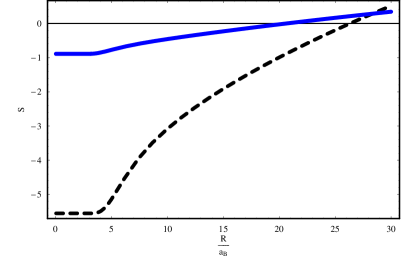
Figure 1: Plots of squeezing versus ration $\frac{r}{a_{B}}$. Solid line correspond to $\frac{\Omega_{0}}{\Omega_{1}}=0.5$, dash line correspond to $\frac{\Omega_{0}}{\Omega_{1}}=0.2$. In both plots Lamb-Dick parameter is chosen as $\kappa=0.3$.

References

- [1] R. J. Glauber, Phys. Rev. 130 (1963) 2529; R. J. Glauber, Phys. Rev. 131 (1963) 2766; R. J. Glauber, Phys. Rev. Lett. 10, 84 (1963).
- [2] J. R. Klauder and B. S. Skagerstam, Coherent states, Applications in Physics and Mathematical Physics (Singapore: World Scientific, 1985).
-
[3]
P. A. Perelomov, Generalized Coherent States and Their
Applications, (Berlin: Springer, 1986).
S. T. Ali, J-P Antoine and J-P Gazeau, Coherent States, Wavelets and Their Generalization, (New York: Springer, 2000). - [4] V. I. Man’ko, G. Marmo, E. C. G. Sudarshan and F. Zaccaria, Phys. Scr. 55, 528 (1997).
- [5] V. I. Man’ko, G. Marmo, E. C. G. Sudarshan and F. Zaccaria, in: N. M. Atakishiev(Ed.), Proc. IV Wigner Symp. (Guadalajara, Mexico, July 1995), World Scientific, Singapore, 1996, P. 427; S. Mancini, Phys. Lett. A 233, 291 (1997); S. Sivakumar, J. Phys. A: Math. Gen. 33, 2289 (2000); B. Roy, Phys. Lett. A 249, 25 (1998); H. C. Fu and R. Sasaki, J. Phys. A: Math. Gen. 29, 5637 (1996); R. Roknizadeh and M. K. Tavassoli, J. Phys. A: Math. Gen. 37, 5649 (2004); M. H. Naderi, M. Soltaolkotabi and R. Roknizadeh, J. Phys. A: Math. Gen. 37, 3225 (2004).
- [6] R. L. deMatos Filho and W. Vogel, Phys. Rev. A 54, 4560 (1996).
- [7] V. I. Man’ko, G. Marmo, A. Porzio, S. Solimeno and F. Zaccaria, Phys. Rev. A 62, 053407 (2000).
- [8] M. H. Naderi, M. Soltanolkotabi and R. Roknizadeh, Eur. Phys. J. D. 32, 397 (2005).
- [9] M. Bagheri Harouni, R. Roknizadeh and M. H. Naderi,
- [10] A. Mahdifar, R. Roknizadeh and M. H. Naderi, J. Phys. A: Math. Gen. 39, 7003 (2006).
- [11] Y. X. Liu, C. P. Sun, S. X. Yu and D. L. Zhou, Phys. Rev. A 63,023802 (2001).
- [12] S. Schmitt-Rink, D. A. B. Miller and D. S. Chemla, Phys. Rev. B 35, 8113 (1987).
- [13] L. Quiroga and N. F. Johnson, Phys. Rev. Lett. 83, 2270 (1999).
-
[14]
G. Chen, N. H. Bonadeo, D. G. Steel, D. Gammon, D.
S. Katzer, D. Park and L. J. Sham, Science 289, 1906
(2000);
M. Bayer, P. Hawrylak, K. Hinzer, S. Fafard, D. Korkushiski, Z. R. Wasilewski, O. Stern and A. Forchel, Science 291, 451 (2001). - [15] Y. X. Liu, S. K. Özdemir, M. Koashi and N. Imoto, Phys. Rev. A 65, 042326 (2002).
- [16] S-K Hong, S. W. Nam and K-H Yeon, Phys. Rev. B 76, 115330 (2007).
- [17] X. Zou, K. Pahlke and W. Mathis, Phys. Rev. A 68, 034306 (2003).
- [18] Ka-Di Zhu, Z-J Wu, X-Z Yuam and Zhen, Phys. Rev. B 71, 135312 (2005).
- [19] F. Tassone and Y. Yamamoto, Phys. Rev. B 59, 1003 (1999).
- [20] I. V. Bondarev, S. A. Maksimenko, G. Ya. Slepyan, I. L. Krestnikov and A. Hoffmann, Phys. Rev. B 68, 073310 (2003).
- [21] E. Hanamura, Phys. Rev B 37, 1273 (1988).
-
[22]
A. D’Andrea and R. Del Sole, Phys. Rev B
41, 1413 (1990);
S. Jazirl, G. Bastard and R. Bennaceur, Semicond. Sci. Tech. 8, 670 (1993). - [23] M. Nirmal, D. J. Norris, M. Kuno, M. G. Bawendi, Al. L. Efros and M. Rosen, Phys. Rev. Lett. 75, 3728 (1995).
-
[24]
M. Sugawara, Phys. Rev. B 51,
10743(1995);
M. Califano, A. Franceschetti, and A. Zunger, Phys. Rev. B 75, 115401 (2007). - [25] P. Machikowski and L. Jacak, Phys. Rev. B 71, 115309 (2005).
- [26] W. Vogel and R. L. de Matos Filho, Phys. Rev. A 52,4214(1995); D. M. Meekhof, C. Monroe, B. E. King, W. M. Itano and D. J. Wineland, Phys. Rev. Lett. 76, 1796(1996).
- [27] R. P. Feynman, Phys. Rev. 84, 108 (1951).
- [28] A. Wojs, P. Hawrylak, S. Fafard and L. Jacak, Phys. Rev. B 54, 5604 (1996).
- [29] M. O. Scully and M. S. Zubairy, Quantum optics, (Cambridge University Press, Cambridge, (1997)).