Particle kinetic analysis of a polar jet from SECCHI COR data

Abstract

Aims. We analyze coronagraph observations of a polar jet observed by the Sun Earth Connection Coronal and Heliospheric Investigation (SECCHI) instrument suite onboard the Solar TErrestrial RElations Observatory (STEREO) spacecraft.

Methods. In our analysis we compare the brightness distribution of the jet in white-light coronagraph images with a dedicated kinetic particle model. We obtain a consistent estimate of the time that the jet was launched from the solar surface and an approximate initial velocity distribution in the jet source. The method also allows us to check the consistency of the kinetic model. In this first application, we consider only gravity as the dominant force on the jet particles along the magnetic field.

Results. We find that the kinetic model explains the observed brightness evolution well. The derived initiation time is consistent with the jet observations by the EUVI telescope at various wavelengths. The initial particle velocity distribution is fitted by Maxwellian distributions and we find deviations of the high energy tail from the Maxwellian distributions. We estimate the jet’s total electron content to have a mass between $3.2\times 10^{14}$ and $1.8\times 10^{15}$ g. Mapping the integrated particle number along the jet trajectory to its source region and assuming a typical source region size, we obtain an initial electron density between $8\times 10^{9}$ and $5\times 10^{10}$ cm^-3 that is characteristic for the lower corona or the upper chromosphere. The total kinetic energy of all particles in the jet source region amounts from $2.1\times 10^{28}$ to $2.4\times 10^{29}$ erg.

1 Introduction

Polar coronal jets were originally observed by the Extreme-Ultraviolet Imaging Telescope (EIT) onboard the Solar and Heliospheric Observatory (SOHO)  (Domingo et al., 1995). In white light, the polar jets discovered by LASCO/SOHO (St. Cyr et al., 1997) appear narrow and collimated, and expand rapidly as they travel through polar regions. They are often associated with an Extreme-Ultraviolet (EUV) jet seen near the solar surface (Wang et al., 1998). These jets are often rooted in bright, low-lying loop features and are similar in appearance to Soft X-ray (SXR) jets (Shibata et al., 1992; Moses et al., 1997). The essential acceleration mechanism for all these jets is very likely provided by magnetic reconnection. The difference between the above and other jet-like features, e.g. chromospheric jets, is the altitude where the magnetic reconnection is assumed to occur. The higher energy jets tend to be accelerated at a higher altitude than the lower energy jets (Shibata et al., 2007). The EUV and SXR jets are often caused by the reconnection in the upper chromosphere or the lower corona.

Wang et al. (1998) analyzed 27 jets in EIT and LASCO data and characterized their motion by three different velocities: the leading-edge velocity $v_{lead}$, the centroid velocity $v_{cen}$ and the initial velocity $v_{init}$ of the centroid. In all cases $v_{cen}$ was much less than $v_{lead}$, indicating that the jets stretched out rapidly as they propagated through the corona. The authors also found that the bulk of the jet material decelerated as it propagated from the limb to the C2 field of view (FOV). This deceleration was attributed to solar gravity. However, the combined results of $v_{init}<v_{escape}$ and $v_{lead}>v_{escape}$, and the lack of evidence for downflow in EIT and C2 led Wang et al. to propose some in situ acceleration that prevents the bulk of the jet material from falling back onto the Sun after it was ejected.

Wood et al. (1999) improved the jet velocity estimates by Wang et al. (1998) using on height-time plots. The authors determined the trace of the jet centroid from the EIT to the C2 FOV and found that the observed kinematic trajectories could be fitted with some success by ballistic orbits. They concluded, however, that gravity alone was not the only force controlling the jet propagation. Because of the similar behavior of the jets studied, both Wood et al. (1999) and Wang et al. (1998) suggested that by the time jets reached the C2 FOV, they were incorporated into the ambient solar wind.

More recently, Ko et al. (2005) studied a jet observed jointly by several instruments above the limb. These authors found that a ballistic model could explain most of the dynamical properties of this jet. In their model it was assumed that the gas was ejected upward from the surface with a range of initial speeds. The smooth change of the upflow-to-downflow speed at a certain altitude derived from the ballistic model was found to be consistent with the change of the line intensities from Doppler dimming observed by UVCS/SOHO. Owing to a lack of high cadence coronagraph observations Ko et al.’s study was essentially confined to heights below 1.64 $r_{\odot}$.

On June 7, 2007 a big eruptive jet was observed by EUVI, COR1, and COR2 on board the STEREO mission with higher spatial and temporal resolution compared to the data from EIT and LASCO C2. It extended from the solar surface to 5 $r_{\odot}$. The event was also studied by Patsourakos et al. (2008) from the stereoscopic viewpoint. They estimated the jet positions and the speed of the leading front at different times in the EUVI FOV.

In this paper we will attempt to analyze the same jet based on white-light coronagraph observations at heights beyond about 1.5 $r_{\odot}$. We extend the ballistic approach by Ko et al. (2005) by quantitatively comparing the density variation from Thomson scattered white-light brightness at different heights to the variation expected from a ballistic model of the jet particles. This method has the advantage that it avoids the estimates of jet centroids and fronts. These fronts are not well-defined for a diffusively spreading plasma cloud, the jet centroids are often difficult to determine because a substantial part of jet material is hidden behind the occulter. Another advantage of our particle kinetic analysis lies is that it also provides a test of the validity of the ballistic model. We therefore receive much more information than the conventional leading edge, centroid velocity measurements. After the description of the observations in §2, we will introduce the ballistic model in §3. In §4 we present the results and try to extrapolate our findings to the jet source region and also discuss the limits of our model. Finally, we summarize our conclusions in the last section.

2 The data

2.1 The polar jet in EUVI, COR1, and COR2 images

The jet we investigated was observed over a radial range from the solar surface out to five solar radii. We used observations from the EUVI and two white light coronagraphs (COR1 and COR2). They belong to the SECCHI instrument suit (Howard et al., 2008). EUVI is a full disk imager with a FOV of 1.7 $r_{\odot}$. COR1 and COR2 are two traditional Lyot coronagraphs, with the FOV in the range of 1.5 $r_{\odot}$ to 4 $r_{\odot}$, and 2.5 $r_{\odot}$ to 15 $r_{\odot}$, respectively. The angular resolution of one pixel in EUVI, COR1, and COR2 is 1.6 arcsec, 7.5 arcsec, and 14 arcsec, respectively.

In EUV, the jet could be observed at all four wavelengths from the EUVI telescope. The time cadence was 10 minutes for 304 Å and 195 Å, and 20 minutes for 284 Å. For 171 Å, the temporal resolution was as high as 2.5 minutes. In Figs. 1 and 2 we show the difference images of the event at four wavelengths of EUVI observed by STEREO A. They were created by subtracting the pre-event images shown in color in the leftmost column of Figs. 1 and 2. The following frames displaying the jet at later times is running from left to right with time. Nearly simultaneous images at different wavelengths are stacked vertically.

The EUVI observations indicate that this jet contains both hot and cool material. The jet eruption first clearly appeared in hotter lines 195 Å and 284 Å at around 05:06 UT, later in 171 Å at around 05:11, and finally in 304 Å at around 05:16 UT. The jet life time appeared to be shorter in the hotter lines (171, 195 and 284 Å), and was clearly longer in the cooler line (304 Å). More detailed descriptions of the EUV observations of this jet are provided in Patsourakos et al. (2008).

Figure 1: The jet time series of difference images at 304 Å, 195 Å and 284 Å from top to bottom observed by the EUVI instrument on board STEREO A.

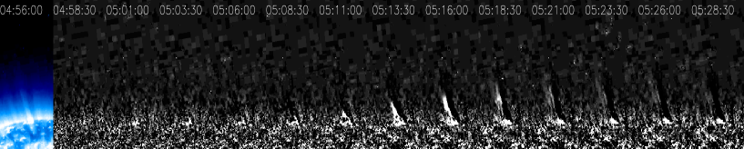
Figure 2: Jet time series of difference images at 171 Å from EUVI A. The FOV is $320^{\prime\prime}\times 672^{\prime\prime}$.

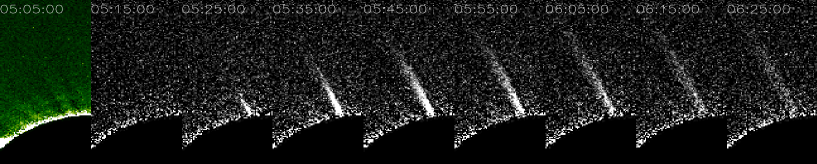
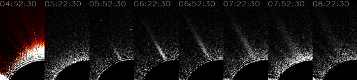
Figure 3: Jet time series of difference total brightness images observed by COR1 (upper row) and COR2 (bottom row) onboard STEREO A. The FOV of each frame in the upper row is $1065^{\prime\prime}\times 2355^{\prime\prime}$, in the bottom row $2744^{\prime\prime}\times 5614^{\prime\prime}$. As a reference, the solar radius was around $1002^{\prime\prime}$ as observed by STEREO A.

Figure 4: Jet geometry in units of Mm trace from EUVI to COR1, then to COR2 (thick curve segments). The thin solid curve is a spline fit to the three traced segments. The half circle indicates the solar limb.

The jet we are studying here was also traced in the COR1 and even in the COR2 field of view. These observations are the main object of our analysis. COR has a polarizer measuring polarized brightness in three directions separated by $120^{\circ}$. From this the total brightness is obtained by the standard procedure $secchi\_prep$. In Fig. 3 we show the total brightness of the jet observations as difference images with respect to the closest pre-event image. Again the images are arranged with observation time from left to right and stacked roughly synchronously for different telescopes.

In Fig 4 the jet geometry traced in the FOV of EUVI, COR1, and COR2 is shown by the three thick curve segments. A smoothing spline is employed to connect the jet orbit over the entire height range. In the next section the trajectory of jet particles is calculated along this thin solid curve in Fig 4. The good alignment of the jet segments from the three instruments indicates that they are part of the same jet. Notice that there was a slight change of about 6 degrees between the jet direction close to the surface as seen in EUVI and at altitudes beyond $1.5\leavevmode\nobreak\ r_{\odot}$ seen in COR1. As a summary, the jet extended out to 5 $r_{\odot}$. The lifetime in EUVI was around several tens of minutes, in COR1 the event could be observed for about 1.5 hours and in COR2 for about 3 hours.

At 171 Å which is the preferred EUV wavelength for plume observations, we noticed a preexisting plume to the right-hand side of the jet. In COR1, the plume was found cospatial with the jet. It is not exceptional that a plume is aligned with a jet in a projected 2D image (Wilhelm et al., 2011). However, this more or less close alignment along the same line of sight (LOS) may be a coincidence. In STEREO B images at 171 Å we also found a preexisting plume slightly to right-hand side of the jet, in COR1 B the plume signal was too faint to conclude that the plume was really close to the jet. In view of the small separation of the two spacecraft of only 10 degrees during this event, we still hesitate to assume that the jet has a physical relation to the preexisting plume. By using difference images, the emission of the plume is eliminated for the subsequent analysis.

2.2 The distance-time brightness relation

Based on the difference images above, we determined the jet intensity in the EUVI images at 304 Å and the white-light total brightness in COR1 and COR2 images for successive times and different distances along the jet axis. The total brightness was integrated across the jet cross section for each exposure and for each position along the jet axis after the pre-event background was subtracted. By integrating the brightness across the jet width, at each distance $s$ the density decrease caused by the magnetic field line divergence was removed. Note that the integration along the line-of-sight direction is implicit in the observation of the optically thin jet plasma. The distance $s$ along the jet axis remains the only relevant spatial coordinate. The resulting distance-time (DT) total brightness plot is shown in Fig. 5. For a clearer view, the brightnesses of COR1 and COR2 in Fig. 5 are multiplied by $10^{9}$ and $10^{10}$, respectively, to match the intensity at 304 Å. Therefore the absolute values in Fig. 5 are not comparable among different instruments. The distance on the ordinate is the length along the jet axis from its footpoint at 1 $r_{\odot}$. The sampling $ds$ in the direction along the jet axis corresponds to the size of one pixel in the respective original images. The time is in units of minutes and starts at $t\,^{{}^{\prime}}_{0}=$ 04:46 UT, which was the earliest observation time of the jet in all frames in Figs. 1, 2, and 3. It ends at 09:21 UT when we were barely able to see a jet signal any more.

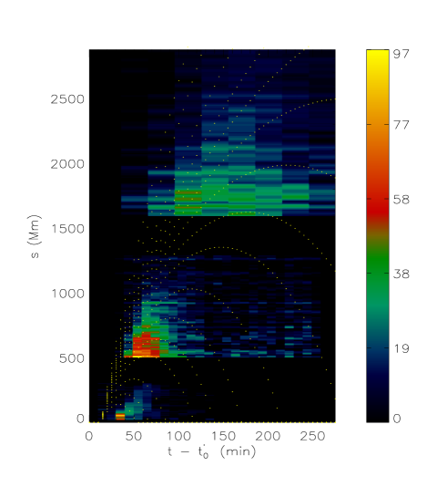
Figure 5: Image intensity for EUVI 304 and brightness for COR1 and COR2 $B(s,t-t\,^{{}^{\prime}}_{0})$ as a function of time and distance along the jet axis. $t\,^{{}^{\prime}}_{0}=$ 04:46 UT, which is a reference time. The intensities and brightnesses were integrated across the jet width from the difference images (Figs.1 and 3). The color code on the right indicates the 304 intensity in units of number of photons. From bottom to top the yellow dotted lines indicate particle trajectories with different initial velocities of 250, 300, 350, 400, 425, 450, 475, 500, 515, 530, 545, 560, 575, 600, 650, and 700 km s^-1.

The white-light signal in COR1 and COR 2 is caused by Thomson scattering at free electrons and therefore the total brightness observed by COR1 and COR2 is proportional to the line-of-sight integrated column density of coronal electrons. Since in Fig. 5 we have subtracted the background and integrated the coronagraph signal across the jet cross section, the resulting image pixel count $B(s,t-t\,^{{}^{\prime}}_{0})\,ds$ for COR1 and COR2 in Fig. 5 is proportional to the number of jet particles at a distance $s$ along the jet in a height range $ds$ resolved by the image pixel, i.e.,

$$B(s,t-t\,^{{}^{\prime}}_{0})\,ds\propto N(s,t-t\,^{{}^{\prime}}_{0})\,ds,$$ (1)

where $N(s,t-t\,^{{}^{\prime}}_{0})ds$ is the number of jet particles in a range $ds$ at a distance $s$ from the foot point of the jet and at a time $t$. $B(s,t-t\,^{{}^{\prime}}_{0})$ is brightness of the corresponding pixel scaled for the different pixel sizes of COR1 and COR2.

3 Ballistic model

For the analysis below, we assumed that in the investigated jet a package of particles ejected upwards with different speeds $v_{0}$ simultaneously during the initiation process. Note that parameter $v_{0}$ is the velocity component parallel to the jet axis. We did not consider the details of the perpendicular velocity, which is related to the gyro motion of particles. Moreover, all particles that move upward follow the jet axis traced in the images from STEREO A. Because we observed the jet very close to the solar limb, we assume that the projection effect does not effect the results much.

3.1 The particle trajectory along the jet

The motion of a charged particle along the unperturbed magnetic field is obtained after averaging the forces over the particle gyro phase

$$\frac{d\tilde{s}}{dt}=\tilde{v}\;,\quad\frac{d\tilde{v}}{dt}=-g_{\odot}\frac{r_{\odot}^{2}}{r(\tilde{s})^{2}}\cos{\alpha(\tilde{s})}-\frac{\mu}{m}\hat{s}\cdot\frac{\partial}{\partial s}\mathbf{B}(\tilde{s})-\mathbf{a}_{\mathrm{coll}}$$ (2)

$$\tilde{s}(0,v_{0})=r_{\odot}\;,\quad\dot{\tilde{s}}(0,v_{0})=v_{0}.$$

Here, $\tilde{s}(t-t_{0},v_{0})$ denotes the distance along the field line and $\tilde{v}(t-t_{0},v_{0})$ the corresponding velocity in which $t_{0}$ is the jet initiation time. The first term on the right-hand side is the gravity force at radius $r(s)$ from the Sun center, $g_{\odot}$ is the gravity on the solar surface and $\alpha$ is the inclination of the local magnetic field that measures the angle between the local radial direction and the tangent of the jet axis. The second term represents the mirror force driven by the particle’s invariant magnetic moment $\mu=mv_{\perp}^{2}/2B$ and the final term accounts for the deceleration of the jet particle by collisions with the background plasma. In the following we ignore the mirror and collision term because they are small at heights above 1.5 $r_{\odot}$ where the coronagraph observations were made. In Sect. 4.3 we justify this choice in more detail and discuss possible modifications from our results concerning the jet properties closer to the surface.

We solved the second-order ordinary differential equation (Equ. 2)numerically by a fourth-order Runge-Kutta method. Each resulting orbit depends on two parameters, the initial velocity $v_{0}$ and the time $t_{0}$ that a particle is ejected from the surface. Because we assumed that the particles were launched in a unique jet event, $t_{0}$ was chosen to be identical for all orbits. Examples of the calculated trajectories for different initial velocities are plotted as dots in Fig. 5 with $v_{0}$ in the range from 250 to 700 km s^-1. The orbit whose apex is close to the edge of the COR1 occulter at a distance of 500 Mm from the surface has the initial velocity 400 km s^-1.

We have overplotted some particle trajectories in Fig. 5 for a somewhat arbitrarily chosen starting time $t_{0}$. Qualitatively, we find that the brightness of a pixel in the DT-diagram is roughly proportional to the number of orbits across it. Because the brightness in white-light coronagraphs is caused by the Thomson scattering and is hence proportional to the electron density, the variation in the jet brightness will be controlled by the particle motion. The distance between particles starting at the same time with different initial velocities will grow continuously according to their orbit $\tilde{s}(t-t_{0},v_{0})$ obtained from Equ. 2. To the extent that the particle position will disperse, the observed brightness of the jet will decrease. This scenario qualitatively agrees with the observations in Fig. 5. In the next section, we quantify this phenomenon.

3.2 The Jacobian

To quantitatively compare the brightness variation caused by the ballistic particle motion to the observations from white light coronagraphs COR1 and COR2, we estimated the jet particle density (Equ. 1) from the particle trajectories (Equ. 2). For this purpose, we equated the number of jet particles $N(s,t-t\,^{{}^{\prime}}_{0})$ in distance range $s$ to $s+ds$ at time $t$ to the number of particles that at time $t_{0}$ were just in the right range of initial velocities $v_{0}$ to $v_{0}+dv_{0}$ to reach the height range $s$ to $s+ds$ at time $t$.

$$N(s,t-t\,^{{}^{\prime}}_{0})\,ds=f(v_{0})\,dv_{0}$$ (3)

Here, $f(v_{0})$ is the initial velocity distribution and $s=\tilde{s}(t-t_{0},v_{0})$ depends on the initial particle velocity. Combining Equ. 1 and 3, we arrive at

$$B(s,t-t\,^{{}^{\prime}}_{0})\propto N(s,t-t\,^{{}^{\prime}}_{0}) = \frac{f(v_{0})}{J(t-t_{0},v_{0})}\;,$$ (4)

$$\quad\mathrm{where}\quad J(t-t_{0},v_{0}) = \frac{d\tilde{s}(t-t_{0},v_{0})}{dv_{0}}$$ (5)

is the Jacobian of the particle orbit. It quantifies the increasing dilution of the particle density along the jet with time. In Fig. 6, an example of $J(t-t_{0},v_{0})$ is plotted vs time for $v_{0}=500$ km s^-1. If initially $v_{0}$ deviates slightly, say $dv_{0}=1$ km s^-1, after a certain time, say 50 mins, the difference in distance along the jet is about 4 Mm because Fig. 6 shows that $J$ at $t-t_{0}=50$ min is about $4\times 10^{3}$ s.

Figure 6: One example of the Jacobian as a function of time for $v_{0}=500$ km s^-1 and $t_{0}=t\,^{{}^{\prime}}_{0}=$ 04:46 UT. $t_{0}$ is the jet initiation time and $t\,^{{}^{\prime}}_{0}$ is the reference time at 04:46 UT.

4 Results and discussions

In this section, the observed brightness distribution $B(s,t-t\,^{{}^{\prime}}_{0})$ along the particle trajectories with given initial velocities $v_{0}$ is fitted by the corresponding Jacobians $J(t-t_{0},v_{0})$ to derive the scaling factors $f(v_{0})$ in Equ. 5 and the optimal jet initiation time $t_{0}$.

4.1 Fit of the Jacobian to the brightness

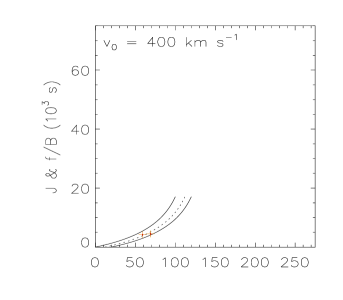
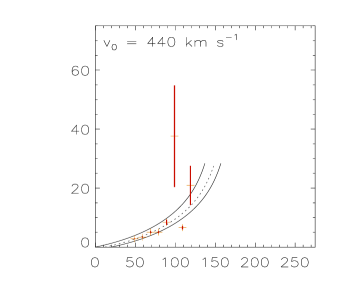
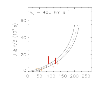
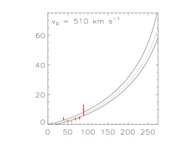
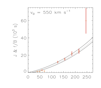
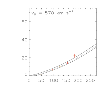
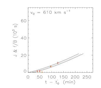
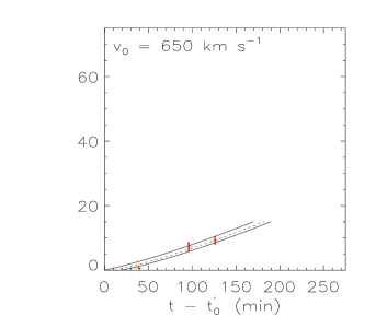
Figure 7: Comparison of the inverse of the observed brightness $B(s,t-t\,^{{}^{\prime}}_{0})$ times a fitted scaling factor $f(v_{0})$ (red vertical bars) and the theoretical Jacobian $J(t-t_{0},v_{0})$ (black dashed curve) as a function of time $t-t\,^{{}^{\prime}}_{0}$ after jet initiation at $t_{0}$. $t\,^{{}^{\prime}}_{0}$ is a reference time at 04:46 UT. The different diagrams are obtained for different initial velocities $v_{0}$, which lead to different particle orbits $s=\tilde{s}(t-t\,^{{}^{\prime}}_{0},v_{0})$ along which $B(s,t-t\,^{{}^{\prime}}_{0})$ is recorded. The vertical range of the red bars indicates the estimated error in $B$. The width between the two solid black curves on both sides of the dased curve shows the variation of $J$ due to an uncertainty in $t_{0}$. For more details see text.

From Equ. 4, we expect the observed $B(s,t-t\,^{{}^{\prime}}_{0})$ to be proportional to the inverse of the theoretical $J(t-t_{0},v_{0})$ for every $v_{0}$ if the correct orbit $s=\tilde{s}(t-t\,^{{}^{\prime}}_{0},v_{0})$ is used in the first argument of $B$ and the initial time $t_{0}$ is chosen correctly. The constant of proportionality, $f(v_{0})$, should then yield the unscaled initial velocity distribution of the jet particles. Since $J(0,v_{0})=0$, we rather use the inverse of Equ. 4 to obtain estimates for $t_{0}$ and $f(v_{0})$ from fits of both sides of the equation. In Fig. 7, we show diagrams for different initial velocities $v_{0}$ of the observed $1/B$ times the fitted scaling factor $f$ (shown as red crosses) in comparison to the theoretical $J$ (black dashed line) for our best estimates of $t_{0}$ and$f(v_{0})$. The initial velocities are chosen to be in the range from 400 to 650 km s^-1.

The uncertainty in $J(t-t_{0},v_{0})$ owing to a possible error in $t_{0}$ is indicated by two solid black curves shifted with respect to the central dashed curve by the uncertainty in the initiation time. The estimated errors of $f/B$ along the respective trajectory $\tilde{s}(t-t\,^{{}^{\prime}}_{0},v_{0})$ are indicated by the vertical range of the red bars. The error estimate was obtained from the noise in the COR1 and COR2 difference images. At each position $s$ along the jet, the noise was calculated according to the standard deviation $\sigma$ of the brightness along a circle centered at the Sun center with its radius reaching the position $s$. In Fig. 7 only data points with a brightness higher than $3\sigma$ are included. The uncertainty of $f/B$ indicated by the red bar represents the $\pm 3\sigma$ levels of the brightness $B$.

The slope of $J(t-t_{0},v_{0})$ at $t\rightarrow t_{0}$ is independent of $v_{0}$. The enhanced slope of $J$ with time reflects the decrease of effective gravity with the distance from the Sun. Particles with higher initial velocities tend to have less dilution of density (smaller slopes for $J$), which is indicated qualitatively in Fig. 5 as well. The plot of curve $J$ in Fig. 7 is terminated either at the time when jet particles hit the solar surface in the cases of low $v_{0}$ or at the time when the particles leave the FOV in Fig. 5 in the cases of high $v_{0}$.

According to Equ. 5, there are two parameters that can be modified to obtain a close fit between $J(t-t_{0},v_{0})$ and $f(v_{0})/B(s,t-t_{0})$. One is the jet initiation time $t_{0}$ which is the same for all diagrams. A change in $t_{0}$ corresponds to a horizontal shift of the red bars in all diagrams simultaneously. Next, there is a scaling factor $f(v_{0})$ for each diagram individually. This factor represents the relative number of particles with this initial velocity in the jet source. Since Equ. 5 still includes a global proportionality constant, the factors $f(v_{0})$ represent only relative number densities at this stage of our analysis. All parameters were optimized for a best fit.

From the EUV observations we conclude that the jet started between 04:46 UT and 05:06 UT. The first clear jet signal was seen at 05:06 UT in 284 Å and 195 Å. There was a small brightening at 04:56 UT as well. However, the signal was too weak to be identified as the jet initiation. Therefore we assume that this jet was ejected in the time range from 04:46 UT to 05:06 UT. This uncertainty is also represented graphically in Fig. 7 by the two solid curves to either side of the central dotted line representing the Jacobian. An initiation time $t_{0}=$ 04:58 UT gives the least sum of the chi-squared deviations for all initial velocities $v_{0}$. We found a three minute uncertainty, which corresponds to the range of $t_{0}$ producing a $\chi^{2}$ enhancement by 5 % above $\chi^{2}_{min}$.

The comparison in Fig. 7 implies that the inverse brightness follows the Jacobian curves quite closely. Although the fit is not perfect, we can say that the ballistic model in general can explain the particle kinematic behavior, and hence the brightness variation in this jet.

4.2 The jet source

As mentioned above, for each $v_{0}$ the fit of $J(t-t_{0},v_{0})$ to $B(s,t-t\,^{{}^{\prime}}_{0})$ yields a scaling factor $f(v_{0})$ that is proportional to the total number of particles with this initial velocity. Therefore, the distribution of $f(v_{0})$ as a function of $v_{0}$ contains information about the initial velocity distribution in the jet source region. This velocity distribution $f(v_{0})$ is shown in Fig. 8 together with a fitted Maxwellian distribution

$$f(v_{0})=C\sqrt{\frac{m}{2\pi\epsilon_{k}}}exp\left[\frac{-m(v_{0}-v_{b})^{2}}{2\epsilon_{k}}\right].$$ (6)

Here $m$ is the averaged atomic mass in the solar corona and approximated as $1.27m_{p}$, $k$ is the Boltzmann constant, $\epsilon_{k}$ is the mean kinetic energy of the particles in the source region and $v_{b}$ a velocity shift of the Maxwellian. Because $f(v_{0})$ is derived from the fit of Jacobian to the observed brightness, it does not refer to the absolute fraction of jet particles with an initial velocity $v_{0}$. However, since brightness is proportional to electron number density, $f(v_{0})$ is thus proportional to the normalized velocity distribution. Therefore, we added a coefficient $C$ in Equ. 6. In the left panel of Fig. 8, the parameters $\epsilon_{k}$ and $v_{b}$ are chosen to obtain the best fit to the observed values of $f(v_{0})$. The fit results in the values of $\epsilon_{k}=2.6\times 10^{-10}$ erg for the mean kinetic energy and $v_{b}=$ 230 km s^-1 for the velocity shift.

Because orbits with an initial velocity below 400 km s^-1 do not reach the field of view of COR1 and COR2, we are lacking $f(v_{0})$ in the velocity range below this threshold. For this reason, our fit is somewhat insensitive in particular to $v_{b}$. We therefore also considered another fit in the right panel where $v_{b}$ is set to zero. We then found a higher mean kinetic energy of $5.4\times 10^{-10}$ erg.

In either case, we found an enhanced higher energy tail at $v_{0}\geq 600$ km s^-1 that cannot be fitted to a Maxwellian. This deviation from a Maxwellian in the jet source distribution may be the result of a specific heating and acceleration process of the jet particles.

Figure 8: Top: the distribution of the scaling factor $f(v_{0})$ as a function of $v_{0}$ in natural logarithm with a fit by the Maxwellian distribution. Bottom: similar to the top one, the fit by the Maxwellian distribution with fixed $v_{b}=0$ km s^-1.

In addition to the jet initiation time and the initial velocity distribution we have determined the absolute mass ejected by the jet. For a white light coronagraph image, the electron column density scattering into each pixel is proportional to the calibrated pixel total brightness. Since we have subtracted the white-light background, only the jet particle density remains from this calculation. Moreover, the brightness in Fig. 5 was also integrated across the jet widths. If we additionally integrate along the distance $s$, we obtain the total number of jet particles visible in the coronagraphs at any one time.

The relations between the image brightness $B$ and the electron density $N_{e}$ were established by Minnaert (1930), van de Hulst (1950) and Billings (1966). For our purposes, we modified them to

$$B=\frac{B_{\odot}}{1-u/3}\frac{\pi\sigma N_{e}dl}{2}[(1-u)(2C-A\sin^{2}\chi)]+u(2D-B\sin^{2}\chi)],$$ (7)

where $B_{\odot}$ is the physical mean solar brightness (MSB) that is used as units in which calibrated COR1 and COR2 observations are expressed. $A,B,C,andD$ are known functions of the distance of the scattering location from the Sun’s center that express the dependence of the scattered polarization on the size of the solar disk as seen from the scatterer. $u$ accounts for the solar disk limb darkening and $\sigma$ is the differential Thomson scattering cross section. For $u$, we used the conventional value of 0.56 for the white-light spectral range. Finally, $N_{e}\,dl$ is the electron column density along the line-of-sight direction through the jet. As an approximation, we assumed that the jet was lying in the plane of sky, so that we have a scattering angle $\chi=90^{\circ}$ for the Thomson scattering.

For the jet observations at $t=$ 05:45 UT when it was most prominent, the total brightness has been integrated across the width, say integrated over $dq$ to derive $B(s,t-t_{0})$, which again was integrated over $ds$ along the jet. If we relate this final integration to Equ. 7, we derive $\int N_{e}dldqds$. The result corresponds to a total number of $1.1\times 10^{37}$ jet particles seen above the occulter at this time instance.

From our trajectory analysis this number is related to the particles in the velocity range of $v_{0}$ from 400 to 600 km s^-1. Depending on the extrapolation in velocity space presented in Fig. 8, we may extend the above particle number estimate to the total number of jet particles. The two cases shown there can be considered as two extreme cases. The total number of jet particles obtained this way will then lie between $1.6\times 10^{38}$ (Fig. 8 left case) and $8.9\times 10^{38}$ (Fig. 8 right case). It corresponds to the jet mass between $3.2\times 10^{14}$ and $1.8\times 10^{15}$ g. Note that these extrapolations must be treated with some care. They rely on the fact that the distribution has a strictly Maxwellian core and even the respective parameters are estimates only based on the observed distribution of the far tail. Also, the resulting particle number may seem large compared to previous estimates merely from coronagraph observations, e.g. the COR 1 data at 05:45 UT, because it includes all particles involved, also those with a low initial velocity $v_{0}$, which are not seen in the coronagraph images at all.

We may use these number estimates to speculate about the particle number density in the source region. If we divide the particle number by a typical source volume $V_{BP}$, we obtain the probable number density at the height where the jet heating and/or acceleration took place. Here, the volume of this jet source region is assumed to be the apparent size of the bright point in the 195 Å pre-event image. We estimate this volume to $2\times 10^{28}$ cm³, which yields an electron density between $8\times 10^{9}$ cm^-3 for the case that the jet was heated and accelerated, and $5\times 10^{10}$ cm^-3 for the case that the jet was only heated. The densities are typical for the upper chromosphere or the low corona and we may conclude that the jet material was heated and possibly accelerated in this height region. Based on the values for $N_{e}$, $\epsilon_{k}$ and $V_{BP}$ above, the total kinetic energy of all jet particles in the source region $E_{k}=(1/2)N_{e}\epsilon_{k}V_{BP}$ can be estimated which was between $2.1\times 10^{28}$ erg and $2.4\times 10^{29}$ erg. This energy is consistent with typical energies for microflares, indeed our estimate lies in the higher energy range of the microflare energy spectrum from $10^{27}$ to $10^{30}$ erg. Again we caution the reader that these numbers are based on the extrapolation of the particle velocity distribution as shown in Fig 8. In particular, we implicitly use $v_{0}=$ 0 km s^-1 as the lower bound of the distribution for jet particles. The uncertainty of this lower bound has a strong impact on the estimated total number of jet particles, less impact on the kinetic energy in the source region.

4.3 Mirror force and collisions

The fits of $J(v_{0},t)$ to $f(v_{0})/B(s,t)$ in Fig. 7 as functions of time $t$ after jet initiation are in general good but not perfect. A good deal of this imperfection can be attributed to image noise, especially for high values of $t$, i.e., low observed brightnesses $B(s,t)$. This could be considered as evidence that the particle orbit is sufficiently well described by the action of the gravity force alone. In this subsection we discuss the terms that we neglected from the full equation (2), the mirror force and collisions, and find out the conditions under which they might become important.

We approximate the Sun’s polar magnetic field by a dipole field. Then the magnetic field strength above the pole is

$$H=H_{\odot}\frac{r^{3}_{\odot}}{r^{3}}\;,\quad\frac{\partial{H}}{\partial{r}}=-3H_{\odot}\frac{r^{3}_{\odot}}{r^{4}}\;,\quad$$ (8)

where $H_{\odot}$ is the field strength at the pole. The mirror force on an individual particle can then be written as $F_{m}=\mu\partial{H}/\partial{r}$ and therefore decreases as $\propto r^{-4}$ with distance from the solar surface. Note that $\mu=mv_{\perp}^{2}/2H$ is the particle’s magnetic moment and an adiabatic invariant of motion provided that the spatial variations of the magnetic field are smooth. On the other hand, the gravity felt by the particle decreases as $\propto r^{-2}$ and hence less rapidly than the mirror force. On the surface of the Sun, comparison of the mirror force and gravity force shows that the latter dominates as long as the local escape velocity $(2g_{\odot}r_{\odot}^{2}/r(s))^{1/2}$ well exceeds the perpendicular velocity $v_{\perp}$. For a thermal speed on the order of the escape velocity of 618 km s^-1, a temperature of 46 MK is required.

The other effect neglected in our analysis are possible collisions of the jet particles with the coronal plasma background. In order to estimate this effect, we used as an estimate of the collisional deceleration $\mathrm{a}_{\mathrm{coll}}$ the friction coefficient of the Fokker-Planck collision term in a kinetic plasma description(e.g., Ishimaru (1973)). The deceleration depends on the velocity $v$ of the jet particle relative to the thermal velocity $v_{\mathrm{therm}}$ of the coronal background, which is assumed at rest. Then for singly charged particles,

$$a_{\mathrm{coll}}(v)=-\mathrm{sign}(v)\;\frac{e^{2}}{m\lambda_{D}^{2}}\ln\Lambda\;G(\frac{v}{v_{\mathrm{therm}}}),$$ (9)

where $e$ is the electron charge, $\lambda_{D}$ the coronal plasma Debye length and $\ln\Lambda$ the respective Coulomb logarithm. An implicit assumption in Equ. 9 is that the background plasma has a Maxwellian velocity distribution. The velocity dependence in the Fokker-Planck collision term generally expressed by Rosenbluth potentials can then be reduced to the Chandrasekhar function (Rosenbluth et al., 1957)

$$G(x)=\frac{1}{2}\frac{d}{dx}(\frac{\mathrm{erf}(x)}{x})$$

The velocity of the jet particles is well ahead of $v_{\mathrm{therm}}$ on a large part of their orbit, therefore $G$ is needed for large arguments for which it decays as $\simeq 1/2x^{2}$. Hence faster particles feel less collisional deceleration, which eventually could lead to a runaway of energetic particles (e.g., Dreicer (1959); Springmann and Pauldrach (1992)).

Figure 9: Top: Electron density assumed for the background corona, adapted from Quémerais & Lamy (2002). Bottom: Collisional deceleration of the jet particles for velocities of 400 to 600 km s^-1 in steps of 50 km s^-1 (solid, from right to left) compared to the gravitational accelaration (dashed).

For our estimates we assumed a density as in the left panel of Fig. 9 adopted from Quémerais & Lamy (2002). In the right panel of Fig. 9 the resulting deceleration $a_{\mathrm{coll}}$ for different velocities and the gravitational acceleration are compared. The neglect of collisions in our analysis is justified above about 1.4 $r_{\odot}$ for particles with 400 km s^-1 and for even lower heights for faster particles. For heights below, the coupling of the jet particles to the background plasma is very intense and a single particle analysis of the jet seems no longer justified.

The effect these collisions will probably have is that part of the jet’s momentum will be transferred to the background plasma, which in turn is accelerated. Therefore not all particles we see above the occulter may be original jet particles, and the distribution function we deduced in Fig. 8 may be the result of some interaction of the original jet with the background plasma. The fact that the distribution in Fig. 8 closely fits to a Maxwellian at lower velocities may be evidence for these collisional processes at lower heights.

In the above collision estimate, we have ignored the solar wind in the distribution of the coronal background particles. We expect that this does not alter our conclusions substantially because below about 1.4 $R_{\odot}$, where collisions matter, the solar wind is probably still subsonic. At greater heights, where the solar wind speed becomes significant, the collisional coupling of the jet particles is scarce.

However, a more serious point is that the acceleration mechanism that drives the solar wind may also affect the jet particles and should then be added as additional term to the right-hand side of Equ. 2. A physical mechanism for this acceleration has, however, not been identified yet and any such acceleration term would be highly speculative.

5 Conclusions

We have followed the evolution of a big eruptive jet event observed by SECCHI in both EUVI images and the COR1 and COR2 white-light coronagraphs. Based on the distance-time brightness analysis, we found that a ballistic model for the jet particles in general can explain quite well the brightness variation beyond 1.5 $r_{\odot}$ in the COR1 and COR2 fields of view with gravity as the dominant acceleration of the jet particles.

Additional parameters were derived or at least estimated, such as the initiation time, the initial velocity distribution, and the number of the jet particles. The derived initiation time is consistent with the EUVI observations at lower altitudes. The initial velocity distribution was fitted by two Maxwellian distributions with different mean kinetic energies. The good agreement with a Maxwellian for lower initial velocities may be due to collisions at heights below 1.4 $r_{\odot}$. At high initial velocities, the distribution deviates from the Maxwellian toward a power law tail that may be a result of the jet acceleration process. The total jet particle number and kinetic energy sum up to about 1.6 to 8.9$\times 10^{38}$ and 2.1 to 24$\times 10^{28}$ erg, respectively.

We neglected the effect of the magnetic mirror force and of Coulomb collision. As discussed, they might have some effect on the kinetics of the jet particles at lower altitudes. Note that these two forces counteract each other: while the collisions with the background plasma will decelerate the particles, the mirror force accelerates them away from the Sun. Especially the correct modeling of the Coulomb collisions below 1.4 $r_{\odot}$ requires additional assumptions, e.g., about the coronal background density and its velocity.

We outlined the basic idea of a new kinetic jet analysis. In the future, a more sophisticated kinetic model of the jet may be compared to white-light observations. We have shown that this comparison allows one to constrain details of the jet which could not be derived in previous studies. More work needs to be done in these directions. Moreover, more jet samples are required to find out to which extent a jet is embedded in the ambient solar wind and how the jet interacts with it.

PROBA-3, which will be launched in a few years, will have a coronagraph with a FOV of 1.04 to 3 $r_{\odot}$. It will provide us with a broader initial velocity coverage because the lower velocity limit depends on the occulter’s size . Therefore we will have less uncertainty in the initial velocity distribution, the electron density in the jet source region, etc. The higher temporal observations with more wavelength coverage from AIA/SDO will help determine the jet initiation time more precisely.

Recently, Raouafi et al. (2008) found that a jet was very often succeeded by a plume above the jet launch site. Interestingly, in our jet study a plume was visible in both EUVI and COR1 before the jet. This phenomenon was also observed by Lites et al. (1999) and other white-light observations in LASCO C2 (Llebaria et al., 2002). However, no definite conclusion is given concerning the relation between plume and jet. A time series of 3D reconstruction of both plume and jet needs to be made to find the answer to this question.