Origin of the GeV emission during the X-ray flaring activity in GRB 100728A

Abstract

Recently, Fermi-LAT detected GeV emission during the X-ray flaring activity in GRB 100728A. We study various scenarios for its origin. The hard spectrum of the GeV emission favors the external inverse-Compton origin in which X-ray flare photons are up-scattered by relativistic electrons in the external forward shock. This external inverse-Compton scenario, with anisotropic scattering effect taken into account, can reproduce the temporal and spectral properties of the GeV emission in GRB 100728A.

1 Introduction

One of the key discoveries by the Swift satellite is the presence of X-ray flares during the early afterglow phase in a large fraction of gamma-ray bursts (GRBs) (see, e.g., Burrows et al. 2005; Zhang et al. 2006; Nousek et al. 2006). The rapid rise and decay behavior of X-ray flares suggests that they are caused by internal dissipation of energy due to late central-engine activity. It was predicted that when the inner flare photons pass through the forward shocks, they will be up-scattered by forward shock electrons, producing a GeV flare (Wang et al. 2006; Galli & Piro 2007; Fan et al. 2008). The angular dispersion effect at the forward shock front will wash out any shorter temporal structure (Beloborodov 2005), so the high-energy inverse-Compton (IC) emission has a much smoother temporal structure determined by the forward shock dynamical time. The incoming X-ray flare photons are anisotropic as seen by the isotropically distributed electrons in the forward shock, so the scatterings between the flare photons and electrons in the forward shock are anisotropic. This effect may decrease the IC emission in the $1/\Gamma$ cone along the direction of the photon beam, where $\Gamma$ is the bulk Lorentz factor of the forward shock, but enhance the emission at larger angles, which leads to a delayed arriving time of the IC photons relative to the flare photons (Wang et al. 2006; Fan et al. 2008). On the other hand, the self inverse-Compton emission of X-ray flares may give rise to a high-energy component which should have similar light curves as the flares (Wang et al. 2006; Fan et al. 2008; Yu & Dai 2009). During the early afterglows, the afterglow synchrotron emission can also produce an extended high-energy component, which is thought to be responsible for the decaying long-lived high-energy emission detected from several GRBs by Fermi/LAT (e.g. Kumar & Barniol Duran 2009, 2010; Ghisellini et al. 2010; Wang et al. 2010; De Pasquale et al. 2010; Corsi et al. 2010; He et al. 2011, Liu & Wang 2011).

GRB 100728A is the second case (after GRB 090510) with simultaneous detections by Swift and Fermi/LAT (Abdo et al. 2011). In this paper, we first analyze the Swift XRT data and the Fermi/LAT data of GRB 100728A, and obtain the X-ray and high-energy ($>$100 MeV) light curves (§2). The early (167-854 seconds) X-ray afterglow exhibits intense and long-lasting flaring activity, with a total of 8 flares (Abdo et al. 2011). Two X-ray flares are also seen at the late stage (80-167 seconds) of the prompt phase (see Fig.1), indicating that the X-ray activity continues from the prompt phase to the afterglow phase. Interestingly Fermi/LAT detected high-energy gamma-ray emission during the X-ray flaring activities (Abdo et al. 2011). These simultaneous X-ray and GeV observations offer a good case to study the nature of high energy emission. In §3, we confront the observations with the theoretical models and find that the external inverse-Compton (EIC) scattering of X-ray flare photons by electrons in the forward shock provides the best explanation for the GeV emission. We calculate the light curve of the EIC emission by taking into account the anisotropic scattering effect, and compare it with that of the observed GeV emission by Fermi/LAT in §4. Finally, we give our conclusions in §5.

2 Observational facts of GRB100728A

Bright GRB 100728A was triggered by both Swift/BAT and Fermi/GBM with $T_{90}\sim 163$ s. Intense X-ray flares are observed by Swift/XRT and significant GeV photons are detected by Fermi/LAT in the meanwhile during the early afterglow phase. Our study mainly focuses on this phase to model both the X-ray and GeV behaviors. The XRT data are reprocessed by our own codes (Zhang, B.-B et al. 2007). Pass 7 LAT data are retrieved from the Fermi LAT data server and reprocessed using a likelihood method. We selected ”transient”(evclass=0) LAT photons during the prompt emission phase and ”source” (evclass=2) LAT photons during the afterglow phase in a 20-degree circular region. The time bins are judged according to the separation among the prompt emission, flare and pure afterglow phases. Our results are generally consistent with Abdo et al. (2011). The observational facts related to our modeling in this work are summarized as follows: i) The burst is bright with a fluence of $\sim 1.3\times 10^{-4}{\rm ergcm^{-2}}$ in 10-1000 keV; ii) Ten successive flares in XRT (from $\sim 80$ s to $\sim 854$ s) are detected, the time-average spectrum of these flares can be described by a Band function with $\alpha=-1.06\pm 0.11$, $\beta=-2.24\pm 0.02$ and a peak energy $\varepsilon_{\rm pk}=1.0^{+0.8}_{-0.4}{\rm keV}$ (Abdo et al. 2011); iii) The spectrum of the GeV emission is hard with a photon index of $\Gamma_{\rm LAT}=-1.4\pm 0.2$ (Abdo et al. 2011); iv) The flux of GeV emission during the time $t\sim 167-854$ s is $F_{\rm LAT}\sim(5.8\pm 4.5)\times 10^{-9}{\rm erg\,cm^{-2}\,s^{-1}}$. In what follows, we investigate which theoretical scenarios can explain these observations.

3 Confronting the observations with various models

3.1 Afterglow synchrotron emission scenario

The underlying X-ray afterglow flux during the flare period should be $F_{\rm X,af}\lesssim 10^{-9}{\rm ergcm^{-2}s^{-1}}$ at time $t\sim 500$ s, according to Fig.1. The post-flare X-ray afterglow has a decay index $\alpha_{2}=1.07\pm 0.05$ before $t\sim 10{\rm ks}$ and an average photon index of $\Gamma_{\rm X}=-2.07\pm 0.09$ (i.e., $\beta_{2}=-1.07\pm 0.09$ for the spectral index in the convention $F_{\nu}\propto t^{\alpha_{2}}\nu^{\beta_{2}}$) (Abdo et al. 2011, Evans $\&$ Cannizzo 2010). Since the temporal index and spectral index satisfy $\alpha_{2}\simeq\frac{3\beta_{2}+1}{2}$, i.e., the closure relation for the afterglow emission in the fast-cooling regime for constant-density interstellar medium (ISM) case (Zhang & Mészáros 2004). The power law index of electron number distribution $p$ ( i.e., $dn_{e}/d\gamma_{e}\propto\gamma_{e}^{-p}$), can then be obtained $p=-2\beta_{2}\simeq 2.2$ (Sari et al. 1998, Zhang $\&$ Mészáros 2004). Thus, extrapolating it to the LAT energies, the GeV flux from the forward shock should be $F_{\rm GeV,af}=F_{\rm X,af}(\rm 1GeV/1keV)^{-\Gamma_{\rm X}+2}\lesssim 0.6\times 10^{-9}{\rm erg\,cm^{-2}\,s^{-1}}$. This flux is about one order of magnitude lower than the observed GeV flux, disfavoring the forward shock synchrotron emission model. Moreover, the hard spectrum of the GeV emission ($\Gamma_{\rm LAT}=-1.4\pm 0.2$, much harder than the X-ray spectrum with $\Gamma_{\rm X}=-2.07\pm 0.09$) cannot be explained by this model.

3.2 X-ray flare self-IC scenario

As argued in Abdo et al. (2011), the LAT emission extends over the flaring period in the early afterglow phase, rather than mainly originated during the higher-significance flares. A cross-correlation analysis between the LAT (diffuse-class) and XRT light curves does not detect any significant temporal correlation or anti-correlation between the two data sets (Abdo et al. 2011). These facts, if true, would disfavor the self-IC scenario for the GeV emission, since this scenario predicts a tight temporal correlation between X-ray flares and GeV flares. However, we should note that the GeV emission signal is not sufficiently strong to allow one to draw a firm conclusion.

The hard GeV spectral shape can be accounted for by a self-IC component only if it peaks in or above the LAT energy window, i.e. $\varepsilon_{\rm p,IC}\gtrsim{\rm 1GeV}$. As the peak energy of the IC emission and the seed photon emission are related by $\varepsilon_{\rm p,IC}\simeq 2\gamma_{\rm m}^{2}\varepsilon_{\rm p,syn}\simeq 2\gamma_{\rm m}^{2}\varepsilon_{\rm pk}$ with the observed peak energy $\varepsilon_{\rm pk}=1.0{\rm keV}$ (Abdo et al. 2011), this requires $\gamma_{\rm m}\gtrsim 700$, where $\gamma_{\rm m}$ is the characteristic Lorentz factor of the electrons. Since the characteristic Lorentz factor of electrons (in the comoving frame) is $\gamma_{\rm m}=1.8\times 10^{3}(p-2)/(p-1)\epsilon_{e}(\Gamma_{\rm sh}-1)$ (Wang et al. 2006), where $\epsilon_{e}$ is the equipartition factor of electrons and $\Gamma_{\rm sh}$ is the Lorentz factor of the internal shock, this would imply $\epsilon_{e}\gtrsim 0.4(p-1)/(p-2)(\Gamma_{\rm sh}-1)^{-1}$. Since the relative shock Lorentz factor may be of order unity (Wang et al. 2006), i.e. $\Gamma_{\rm sh}\sim 1-2$, the inferred value of $\epsilon_{e}$ is $\epsilon_{e}\gtrsim 1$ for $p\simeq 2-3$, which is too large to be realistic. We note that this scenario can not be excluded if the Lorentz factors ($\Gamma_{\rm sh}$) of the internal shocks for these X-ray flares are very large.

3.3 The external IC scenario

The hard spectrum can be more easily accounted for in an external IC (EIC) scenario, in which the flare photons are scatterred by external forward shock electrons. This is because the Lorentz factors of the electrons in the forward shock are larger by a factor of $\Gamma$ (i.e., the bulk Lorentz factor of the forward shock), compared to the internal shock case, and hence the EIC emission peaks at much higher energies. In the adiabatic case, the shock Lorentz factor can be derived by

$$\Gamma=44E_{53}^{1/8}n_{0}^{-1/8}t_{3}^{-3/8},$$ (1)

where we use the convention $Q_{x}=Q/10^{x}$ in cgs units hereafter (Sari et al. 1998). Adopting equation (1), we can obtain the typical Lorentz factor of the post-shock electrons at time $t$ as $\gamma_{\rm m}\simeq 1.8\times 10^{3}(p-2)/(p-1)\epsilon_{e}\Gamma=1.3\times 10^{3}\epsilon_{e,-1}f_{p}E_{53}^{1/8}n_{0}^{-1/8}t_{3}^{-3/8}$, where $f_{p}\equiv\frac{6(p-2)}{(p-1)}$, $E$ is the kinetic energy of the blast wave and $n$ is the number density of the circum-burst medium. By inputting the value of the observed peak energy $\varepsilon_{\rm pk}=1.0{\rm keV}$ (Abdo et al. 2011) into $h\nu_{\rm m}^{\rm EIC}=2\gamma_{\rm m}^{2}\varepsilon_{\rm pk}$ (Sari $\&$ Esin 2001, Wang et al. 2006), we can obtain the peak of the observed EIC $\nu F_{\nu}$ flux as

$$h\nu_{\rm m}^{\rm EIC}=4\times 10^{9}{\rm eV}\epsilon_{e,-1}^{2}E_{53}^{1/4}n_{0}^{-1/4}t_{3}^{-3/4}$$ (2)

for $p=2.2$.

The high flux of the X-ray flares will result in enhanced cooling of the electrons in the forward shock. Adopting equation (1) and the shock radius as $R=4\Gamma^{2}ct$(Waxman 1997), the energy density of X-ray flare photons in the forward-shock frame is

$$\begin{array}[]{ll}U_{\rm X}^{\prime}=d_{\rm L}^{2}F_{\rm X}/(\Gamma^{2}R^{2}c)\\ =0.34E_{53}^{-3/4}n_{0}^{3/4}F_{{\rm X},-8}d_{\rm L,28}^{2}t_{3}^{1/4}{\rm erg\,s^{-1}\,cm^{-2}},\end{array}$$ (3)

where $F_{\rm X}$ is the observed flare flux, $d_{\rm L}$ is the luminosity distance of the burst. Considering the case in which EIC cooling is dominant, the cooling power is $P(\gamma_{e})=\frac{4}{3}\sigma_{T}c\Gamma^{2}\gamma_{e}^{2}U_{\rm X}^{\prime}$ (Sari et al. 1998), then the cooling Lorentz factor of electrons can be obtained by equation $\Gamma\gamma_{c}m_{e}c^{2}=P(\gamma_{c})t$ (Sari et al. 1998), i.e.,

$$\begin{array}[]{ll}\gamma_{\rm c}\simeq 3m_{e}c^{2}/(16\sigma_{\rm T}cU_{\rm X}^{\prime}\Gamma t)\\ =5\times 10^{2}E_{53}^{5/8}n_{0}^{-5/8}F_{\rm X,-8}^{-1}d_{\rm L,28}^{-2}t_{3}^{-7/8}.\end{array}$$ (4)

Thus, adopting equation (4) and $\varepsilon_{\rm pk}=1.0{\rm keV}$, the cooling break in the EIC spectrum can be obtained as (Sari $\&$ Esin 2001, Wang et al. 2006)

$$\begin{array}[]{ll}h\nu_{\rm c}^{\rm EIC}=2\gamma_{\rm c}^{2}\varepsilon_{\rm pk}\\ =5\times 10^{8}{\rm eV}E_{53}^{5/4}n_{0}^{-5/4}t_{3}^{-7/4}F_{\rm X,-8}^{-2}d_{\rm L,28}^{-4}.\end{array}$$ (5)

Below $\nu_{\rm m}^{\rm EIC}$, the EIC spectrum has a photon index of $\Gamma_{\rm EIC}=-3/2$ if $\nu_{\rm c}^{\rm EIC}<\nu<\nu_{\rm m}^{\rm EIC}$, or has the same index as the low-energy index ($\alpha=-1.06\pm 0.11$) of the X-ray flare spectrum if $\nu<\min(\nu_{\rm c}^{\rm EIC},\nu_{\rm m}^{\rm EIC})$ (Sari $\&$ Esin 2001, Wang et al. 2006). Therefore, below $\nu_{\rm m}^{\rm EIC}$, the photon index of the EIC emission is consistent with the hard spectrum of the observed GeV emission, $\Gamma_{\rm LAT}=-1.4\pm 0.2$.

Using $R=4\Gamma^{2}ct$ for the radius of the forward shock and the spectral peak $\varepsilon_{\rm pk}=1.0\rm keV$ (Abdo et al. 2011), we can derive the peak spectral flux of the EIC emission as (Sari $\&$ Esin 2001)

$$\begin{array}[]{ll}f_{\rm p}^{\rm EIC}=\tau_{\rm ssc}\left(\frac{F_{\rm X}}{\varepsilon_{\rm pk}}\right)k_{a}=\frac{1}{3}\sigma_{\rm T}nR\left(\frac{F_{\rm X}}{\varepsilon_{\rm pk}}\right)k_{a}\\ =2\times 10^{-33}k_{a}E_{53}^{1/4}n_{0}^{3/4}t_{3}^{1/4}F_{\rm X,-8}{\rm erg\,cm^{-2}\,s^{-1}\,Hz^{-1}},\end{array}$$ (6)

where $\tau_{\rm ssc}=\frac{1}{3}\sigma_{\rm T}nR$ is the scattering optical depth of the forward shock shell, $\sigma_{\rm T}$ is the Thompson cross section, $k_{a}$ is the correction factor accounting for the suppression of the IC flux due to the anisotropic scattering effect compared to the isotropic scattering case. It is found that this correction is mild with $k_{a}\sim 0.4$ (Fan & Piran 2006; He et al. 2009).

Therefore, the peak flux of the EIC emission for the fast cooling case (i.e., $\nu_{\rm c}^{\rm EIC}<\nu_{\rm m}^{\rm EIC})$ is (Sari $\&$ Esin 2001)

$$\begin{array}[]{ll}\nu_{\rm m}^{\rm EIC}f_{\rm m}^{\rm EIC}=\nu_{\rm m}^{\rm EIC}f_{\rm p}^{\rm EIC}\left(\frac{\nu_{\rm m}^{\rm EIC}}{\nu_{\rm c}^{\rm EIC}}\right)^{-1/2}\\ =7\times 10^{-10}k_{a}E_{53}\epsilon_{e,-1}t_{3}^{-1}d_{L,28}^{-2}{\rm erg\,s^{-1}\,cm^{-2}}.\end{array}$$ (7)

From the spectrum of the observed GeV emission at $t=10^{3}{\rm s}$, we have two constraints, i.e.,

$$h\nu_{\rm m}^{\rm EIC}\gtrsim 10^{9}{\rm eV},$$ (8)

and

$$\nu_{\rm m}^{\rm EIC}f_{\rm m}^{\rm EIC}\sim 5\times 10^{-10}{\rm erg\,cm^{-2}\,s^{-1}}.$$ (9)

Inputting equations (2) and (7) into the above two constraints, respectively, one can get the following constraints

$$n_{0}^{1/4}\lesssim 4E_{53}^{1/4}\epsilon_{e,-1}^{2}$$ (10)

and

$$\epsilon_{e}\sim 0.07k_{a}^{-1}E_{53}^{-1}d_{\rm L,28}^{2}.$$ (11)

The above constraints are consistent with the post-flare X-ray afterglow observations. We attribute the post-flare X-ray afterglow to the synchrotron forward shock emission. Since its temporal index and spectral index satisfy the closure relation $\alpha_{2}=\frac{3\beta_{2}+1}{2}$, as mentioned in section 3.1, the X-ray afterglow emission is in the fast cooling regime. According to equation (9) in Zhang et al. (2007), the synchrotron X-ray afterglow flux is

$$\begin{array}[]{ll}\nu F_{\nu}^{\rm XRT}=2\times 10^{-11}{\rm erg\,s^{-1}\,cm^{-2}}\\ \epsilon_{e,-1}^{p-1}\epsilon_{B,-2}^{\frac{(p-2)}{4}}E_{53}^{\frac{(p+2)}{4}}\times g_{p}(1+Y)^{-1}t_{4}^{(2-3p)/4}\nu_{18}^{(2-p)/2}D_{\rm L,28}^{-2},\end{array}$$ (12)

where $g_{p}=8.6\left(\frac{p-2}{p-1}\right)^{p-1}(3.3\times 10^{-5})^{\frac{p-2.2}{2}}$, and the IC parameter is $Y=(-1+\sqrt{1+4\eta\epsilon_{e}/\epsilon_{B}})/2$ with $\eta$ being the radiation efficiency (Sari $\&$ Esin 2001). According to Sari et al. (1998), the afterglow cooling Lorentz factor of electrons is $\gamma_{c}^{\rm af}=1.6\times 10^{3}E_{53}^{-3/8}n_{0}^{-5/8}\epsilon_{B,-1}^{-1}t_{4}^{1/8}(1+Y)^{-1}$. If the IC parameter $Y$ is not too large, we have $\gamma_{c}^{\rm af}>\gamma_{m}$ at $t\sim 10^{4}{\rm s}$, implying a slow cooling case, where the radiation efficiency is $\eta=(\gamma_{c}^{\rm af}/\gamma_{m})^{2-p}=0.8h_{p}E_{53}^{2-p}n_{0}^{(p-2)/2}\epsilon_{B,-1}^{p-2}\epsilon_{e,-1}^{p-2}t_{4}^{(2-p)/2}(1+Y)^{p-2}$ with $h_{p}=1.1^{2.2-p}$ (Sari $\&$ Esin 2001). At $t=10^{4}$ s, for $D_{L}=2\times 10^{28}{\rm cm}$ (i.e., at redshift $z$=1), with $\epsilon_{e}\sim 0.3$, $\epsilon_{B}\sim 0.1$, $n=1{\rm cm^{-3}}$ and $E\sim 3\times 10^{53}{\rm erg}$, the IC parameter is $Y\simeq 1$. For the above parameters, the flux derived from equation (12) is consistent with the observed X-ray flux $\nu F_{\nu}^{\rm XRT}\sim 3\times 10^{-11}{\rm erg\,cm^{-2}\,s^{-1}}$.

Note that in the above estimate we have implicitly assumed that the X-ray flare flux is sufficiently strong that the electrons in the forward shocks are cooled down by the flare photons (i.e. $\gamma_{\rm m}>\gamma_{\rm c}$). Nevertheless, in the regime that electrons cool slowly ( i.e., $\gamma_{\rm m}<\gamma_{\rm c}$ in the slow cooling case), one can also have an EIC spectrum as hard as the low-energy spectrum of the X-ray flare (i.e., $\Gamma_{\rm EIC}\simeq\alpha=-1.06\pm 0.11$) if $h\nu_{\rm m}^{\rm EIC}\gtrsim 1{\rm GeV}$. Such a situation will be included in the numerical modelings in §4.

3.4 The afterglow synchrotron self-Compton emission scenario

Predictions were made that the synchrotron self-Compton (SSC) emission from the forward shock electrons can produce GeV emission during the early afterglow in some parameter space (e.g. Zhang & Mészáros 2001). In the case of GRB 100728A, however, the illumination by X-ray flare photons enhances the cooling of the forward-shock electrons, which in turn suppresses the afterglow synchrotron and SSC emission. We expect that the ratio of the EIC luminosity to the SSC luminosity is ${L_{\rm EIC}}/{L_{\rm SSC}}={U^{\prime}_{\rm X}}/{U^{\prime}_{\rm syn}}$, where $U^{\prime}_{\rm X}$ and ${U^{\prime}_{\rm syn}}$ are, respectively, the energy density of flare photons and synchrotron photons in the comoving frame of the forward shocks. During the flare activity period, because the flux of flare photons is significantly larger than that of the synchrotron X-ray afterglow, i.e. ${U^{\prime}_{\rm X}}>{U^{\prime}_{\rm syn}}$, the SSC emission should be subdominant compared to the EIC emission.

4 Numerical modeling of the GeV emission

In this section we calculate numerically the flux of the EIC emission of the x-ray flare photons scattered by forward shock electrons, taking into account the anisotropic scattering effect. For a photon beam penetrating into the shock region where electrons are isotropically distributed, the EIC emissivity of radiation scattered at an angle $\theta_{\rm SC}$ relative to the direction of the photon beam in the shock comoving frame is (Aharonian $\&$ Atoyan1981, Brunetti 2000, Fan et. al. 2008, He et al. 2009):

$$\begin{array}[]{ll}\varepsilon^{\prime\rm EIC}(\nu^{\prime},\cos\theta_{\rm SC})\approx\frac{3\sigma_{\rm T}c}{16\pi}\int^{\gamma_{\rm max}}_{\gamma_{\rm m}}d\gamma_{e}\frac{dn_{e}}{d\gamma_{e}}\int^{\nu^{\prime}_{\rm s,max}}_{\nu^{\prime}_{\rm s,min}}\frac{f^{\prime\rm X}_{\nu^{\prime}_{\rm s}}d\nu^{\prime}_{\rm s}}{\gamma_{e}^{2}\nu^{\prime}_{\rm s}}\\ \left[1+\frac{\xi^{2}}{2(1-\xi)}-\frac{2\xi}{b_{\theta}(1-\xi)}+\frac{2\xi^{2}}{b_{\theta}^{2}(1-\xi)^{2}}\right],\end{array}$$ (13)

where $\nu^{\prime}_{\rm s}$ and $\nu^{\prime}$ are respectively the comoving-frame frequencies of the photons before scattering and after scattering, $\gamma_{e}$ is the Lorentz factor of scattering electrons, $\xi\equiv h\nu^{\prime}/(\gamma_{e}m_{e}c^{2})$, $b_{\theta}\equiv 2(1-\cos\theta_{\rm SC})\gamma_{e}h\nu^{\prime}_{\rm s}/(m_{e}c^{2})$, and $h\nu^{\prime}_{\rm s}\ll h\nu^{\prime}\ll\gamma_{e}m_{e}c^{2}b_{\theta}/(1+b_{\theta})$. Integrating equation (13) over the angle $\theta_{\rm SC}$ for the whole solid angle, one can reduce equation (13) to the equation for the case of isotropically distributed electrons and photons. The maximum Lorentz factor of electrons $\gamma_{\rm max}$ is obtained by equating the electron acceleration timescale to the cooling (including synchrotron cooling and IC cooling) timescale. $f_{\nu^{\prime}_{\rm s}}^{{}^{\prime}\rm X}$ is the flux density of seed photons at the frequency $\nu^{\prime}_{\rm s}$, which are X-ray flare photons in our case. The lowest and highest frequencies of seed photons in the shock frame can be calculated via $\nu^{\prime}_{\rm s,min}=0.3{\rm keV}/\Gamma$ and $\nu^{\prime}_{\rm s,max}=10{\rm keV}/\Gamma$, according to the observation range of Swift XRT, i.e., $0.3{\rm keV}-10{\rm keV}$. The light curves of these X-ray flares are modeled by power-law rises and decays in the calculation, as shown by the green lines in Fig.1 and Fig.2. The spectra of these X-ray flares are modeled by the Band function as given in section 2.

The electron distribution $dn_{e}/d\gamma_{e}$ in Eq.(13) depends on where the cooling break $\gamma_{\rm c}$ is. When the circum-burst density is sufficiently low, the forward shock electrons suffer from weak cooling by X-ray flares, so we have $\gamma_{\rm m}<\gamma_{\rm c}$. Otherwise, we have $\gamma_{\rm m}>\gamma_{\rm c}$. The distribution of electrons is given by (Sari et al. 1998)

$$\frac{dn_{e}}{d\gamma_{e}}\propto\left\{\begin{array}[]{ll}\gamma_{e}^{-2},&\gamma_{\rm c}\leq\gamma_{e}\leq\gamma_{\rm m}\\ \gamma_{e}^{-p-1},&\gamma_{\rm m}<\gamma_{e}<\gamma_{\rm max}\end{array}\right.$$ (14)

for $\gamma_{\rm c}\leq\gamma_{\rm m}\lesssim\gamma_{\rm max}$, and

$$\frac{dn_{e}}{d\gamma_{e}}\propto\left\{\begin{array}[]{ll}\gamma_{e}^{-p},&\gamma_{\rm m}\leq\gamma_{e}\leq\gamma_{\rm c}\\ \gamma_{e}^{-p-1},&\gamma_{\rm c}<\gamma_{e}<\gamma_{\rm max}\end{array}\right.$$ (15)

for $\gamma_{\rm m}<\gamma_{\rm c}\lesssim\gamma_{\rm max}$.

The flux density of the EIC emission at a frequency $\nu$ is given by (Huang et al. 2000, Yu et al. 2007)

$$F_{\nu}^{\rm EIC}=\int^{\theta_{\rm j}}_{0}\frac{\varepsilon^{\prime\rm EIC}(\nu/D,\cos\theta)D^{2}}{d_{\rm L}^{2}}2\pi R^{3}\sin{\theta}\cos{\theta}d\theta,$$ (16)

where $D=1/[\Gamma(1-\beta\cos\theta)]$ is the Doppler factor, $\beta$ is the velocity of the forward shock, $\theta$ is the angle between the motion of the emitting material and the jet axis, and $\theta_{\rm j}$ is the opening angle of the jet. Since $\theta$ also represents the angle between the injecting photons and the observed scattered photons in the observer frame, it is related with the angle $\theta_{\rm SC}$ in the comoving frame by $\cos\theta_{\rm SC}=(\cos\theta-\beta)/(1-\beta\cos\theta)$. $\theta_{\rm j}$ is a function of time with an initial value of $\theta_{\rm j,0}$. Since the integration of Eq. (13) is performed over the equal arrival time surface (EATS), the radius $R$ of the shock is a function of $\theta$, which is determined by

$$t=\int\frac{1-\beta\cos{\theta}}{\beta c}dR\equiv{\rm constant}$$ (17)

within the jet boundaries (e.g. Waxman 1997; Granot et al. 1999).

The calculated light curves and spectra of the EIC emission are shown in Fig.1 and Fig.2 for high ($n=1{\rm cm^{-3}}$) and low ($n=0.01{\rm cm^{-3}}$) circumburst density cases respectively, in which the electron distribution is, correspondingly, in the fast-cooling and slow-cooling regime. In both cases, the EIC emission is the dominant component at GeV energies during the X-ray flare activity period. In the high density case (Fig.1), the electrons are in the fast cooling regime during the X-ray flare period and we have $\nu_{\rm c}^{\rm EIC}<\nu_{\rm LAT}<\nu_{\rm m}^{\rm EIC}$, leading to a hard GeV emission spectrum with a photon index $\Gamma_{\rm GeV}=-1.5$, as shown by the inset spectra of Fig. 1. In contrast to the high temporal variability of the x-ray flares, the EIC emission is very smooth. It is clearly seen that the EIC emission starts later than the earliest flares, which can explain the non-detection of GeV emission during the earliest two flares (80-167s). The EIC emission continues after the X-ray flare activity shuts off, which may explain the marginal detection of GeV emission after the X-ray flare activity, as reported in Abdo et al. (2011).

Fig.2 shows the case of a low circumburst density with $n=0.01{\rm cm^{-3}}$. In this case, a large shock radius results in a lower flare photon density in the shock comoving frame so that the EIC cooling is not important. In this case, we will have $\gamma_{m}<\gamma_{c}$, and thus $\nu_{\rm LAT}<\nu_{\rm m}^{\rm EIC}<\nu_{\rm c}^{\rm EIC}$. The spectrum of the EIC emission below $\nu_{\rm m}^{\rm EIC}$ has the same slope as that of the seed photons, i.e. the photon index is similar to the low-energy photon index $\alpha$ of the Band function describing the spectrum of X-ray flares. Such a spectrum is also consistent with the measured spectrum of the GeV emission within the error bars, as shown in the inset plot of Fig.2. In the low density case, the afterglow synchrotron emission dominates over the SSC emission in the GeV band in the early time.

5 Conclusions

For the first time, GeV emission from a GRB during the X-ray flaring activity has been detected by the Fermi/LAT, in GRB100728A. The temporal coincidence between the GeV emission and the X-ray flares suggests that the GeV emission should be related to the flares in some way. Here we have shown that an EIC scenario, where X-ray flare photons are up-scattered by electrons in the external forward shocks, provides the best explanation for the GeV emission, supporting the earlier prediction of GeV emission from GRB X-ray flares (Wang et al. 2006). The hard spectrum of the GeV emission can be readily explained by the EIC emission. The delayed behavior of the GeV emission relative to the X-ray flares also naturally arises in the EIC scenario. Synergistic observations between Swift and Fermi should be able in the future to find other similar cases, allowing further tests of this EIC scenario.

We are grateful to Bing Zhang and Zigao Dai for valuable discussions. This work is supported by the NSFC under grants 10973008 and 11033002, the 973 program under grant 2009CB824800, the program of NCET, the foundation for the Authors of National Excellent Doctoral Dissertations of China, Jiangsu Province Innovation for PhD candidate CXZZ11$\_$0031, the Fok Ying Tung Education Foundation, NASA NNX08AL40G and NSF PHY 0757155. It is also supported in part by NASA via the Smithsonian Institution grant SAO SV4-74018,A035 [BBZ] at PSU.

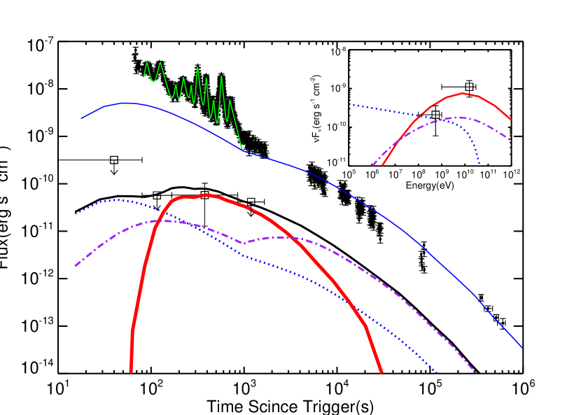
Figure 1: Light curves of the GeV emission and X-ray afterglow of GRB100728A. The filled black squares represent the observed X-ray flux by Swift XRT (0.3-10keV) and the empty black squares represent the high energy data and upper limits from Fermi/LAT ($100{\rm MeV}-30{\rm GeV}$). The green solid line represents the input light curve of X-ray flares that we used in the calculation. The blue solid line represents the synchrotron afterglow emission in 0.3-10 keV, while the red solid line represents the high energy emission (in $100{\rm MeV}-30{\rm GeV}$) produced by the external inverse-Compton scattering of the X-ray flare photons. The blue dotted line and purple dash-dotted line represent, respectively, the afterglow synchrotron emission and the afterglow SSC emission in $100{\rm MeV}-30{\rm GeV}$. The black solid line is the sum of the three high energy components (represented by the red solid line, blue dotted line and purple dash-dotted line, respectively). For clearness, we re-scaled the flux of all the high-energy components by multiplying a factor of $0.01$. The inset plot shows the spectra of the three high-energy components and the LAT data taken from Abdo et al. (2011) during the X-ray flaring period (167-854 s). $E=3\times 10^{53}{\rm erg},n=1{\rm cm^{-3}},p=2.2,\Gamma=250,\theta_{\rm j,0}=0.1,\epsilon_{e}=0.1,\epsilon_{B}=0.04$ and $z=1$ are used in the calculation.

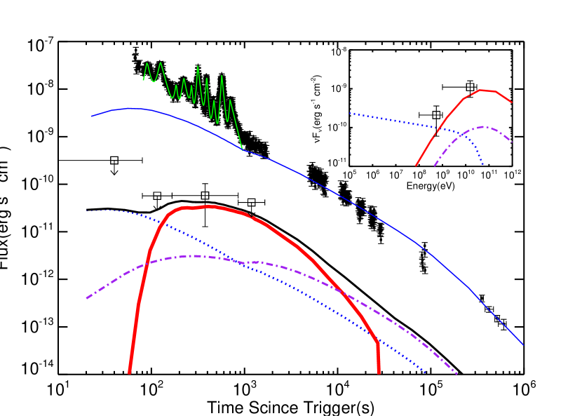
Figure 2: The same as Figure 1, but for a low-density case ($n=0.01{\rm cm^{-3}}$). $E=1\times 10^{53}{\rm erg},n=0.01{\rm cm^{-3}},p=2.2,\Gamma=400,\theta_{j,0}=0.07,\epsilon_{e}=0.2,\epsilon_{B}=0.1$ and $z=1$ are used in the calculation.

References

- (1) Abdo, A. A. et al. 2011, ApJ, 734, L27
- (2) Aharonian, F. A., & Atoyan, A. M. 1981, Ap&SS, 79, 321
- (3) Beloborodov, A. M. 2005, ApJ, 618, L13
- (4) Brunetti, G. 2000, Astroparticle Physics, 13, 107
- (5) Burrows, D. N. et al. 2005, Science, 309, 1833
- (6) Corsi, A., Guetta, D., & Piro, L. 2010, ApJ, 720, 1008
- (7) De Pasquale, M., et al. 2010, ApJ, 709, L146
- Evans & Cannizzo (2010) Evans, P. A., & Cannizzo, J. K. 2010, GRB Coordinates Network, 11014, 1
- (9) Galli, A. & Piro, L, 2007, A&A, 475, 421
- (10) Ghisellini et al. 2010, MNRAS, 403, 926G
- (11) Granot J., Piran T., Sari R., 1999, ApJ, 513, 679
- (12) Fan, Y., & Piran, T. 2006, MNRAS, 370, L24
- (13) Fan, Y.-Z., Piran, T., Narayan, R., & Wei, D.-M. 2008, MNRAS, 384, 1483
- (14) He, H. N., Wang, X. Y., Yu, Y. W., & Mészáros , P. 2009, ApJ, 706, 1152
- (15) He, H. N.; Wu, X. F., Toma, K.; Wang, X. Y. & Mészáros , P., 2011, ApJ, 733, 22
- Huang et al. (2000) Huang, Y. F., Gou, L. J., Dai, Z. G., & Lu, T. 2000, ApJ, 543, 90
- (17) Kumar, P. & Barniol Duran, R., 2009, MNRAS, 400, L75
- (18) Kumar, P. & Barniol Duran, R., 2010, MNRAS, 409, 226
- (19) Liu, R. Y. & Wang, X. Y., 2011, ApJ, 730, 1
- (20) Nousek, J. A. et al. 2006, ApJ, 642, 389
- Sari et al. (1998) Sari, R., Piran, T., & Narayan, R. 1998, ApJ, 497, L17
- Sari & Esin (2001) Sari, R., & Esin, A. A. 2001, ApJ, 548, 787
- (23) Wang, X. Y., Li, Z., & Mészáros , P. 2006, ApJ, 641, L89
- (24) Wang, X. Y., He, H. N. et al., 2010, ApJ, 712, 1232
- (25) Waxman, E. 1997, ApJ, 491, L19
- Yu et al. (2007) Yu, Y. W., Liu, X. W., & Dai, Z. G. 2007, ApJ, 671, 637
- (27) Yu, Y. W. & Dai, Z. G., 2009, ApJ, 692, 133
- Zhang & Mészáros (2004) Zhang, B., & Mészáros, P. 2004, International Journal of Modern Physics A, 19, 2385
- (29) Zhang, B. B.; Liang, E. W.; Zhang, B., 2007, ApJ, 666, 1002
- (30) Zhang, B. et al. 2007, ApJ, 655, 989
- (31) Zhang, B., & Mészáros , P. 2001, ApJ, 559, 110