The Widom line and noise power spectral analysis of a supercritical fluid

Abstract

We have performed extensive molecular dynamics simulations to study noise power spectra of density and potential energy fluctuations of a Lennard-Jones model of a fluid in the supercritical region. Emanating from the liquid-vapor critical point, there is a locus of isobaric specific heat maxima, called the Widom line, which is often regarded as an extension of the liquid-vapor coexistence line. Our simulation results show that the noise power spectrum of the density fluctuations on the Widom line of the liquid-vapor transition exhibits three distinct $1/f^{\gamma}$ behaviors with exponents $\gamma$= 0, 1.2 and 2, depending on the frequency $f$. We find that the intermediate frequency region with an exponent $\gamma\sim$ 1 appears as the temperature approaches the Widom temperature from above or below. On the other hand, we do not find three distinct regions of $1/f^{\gamma}$ in the power spectrum of the potential energy fluctuations on the Widom line. Furthermore, we find that the power spectra of both the density and potential energy fluctuations at low frequency have a maximum on the Widom line, suggesting that the noise power can provide an alternative signature of the Widom line.

I Introduction

In a typical pressure-temperature $(P-T)$ phase diagram for a fluid, there is a first order phase transition line between the liquid and the vapor phases that terminates at a critical point Stanley (1971). Beyond this critical point lies the supercritical regime where one can go continuously between the liquid and vapor phases. In this region thermodynamic response functions such as the isobaric specific heat $c_{p}$, the isothermal compressibility $\kappa_{T}$ and the thermal expansion coefficient $\alpha$ do not monotonically increase or decrease with $P$ and $T$. Rather they exhibit a line of maxima Nishikawa et al. (2003); Brazhkin and Ryzhov (2011); Brazhkin et al. (2011) emanating from the critical point that is known as the Widom line Xu et al. (2005) which can be thought of as an extension of the liquid-vapor phase boundary.

More generally, a Widom line is regarded as an extension of a first order phase boundary that terminates at a critical point. It is marked by maxima in the thermodynamic response functions. The most studied Widom line is in supercooled water where a first order liquid-liquid transition has been proposed between a high-density liquid and a low-density liquid phase Poole et al. (1992); Mishima and Stanley (1998); Soper and Ricci (2000). This phase boundary has been hypothesized to end in a critical point from which the Widom line emanates Poole et al. (1992); Mishima and Stanley (1998); Xu et al. (2005). This critical point cannot be directly investigated experimentally because it is usurped by the spontaneous crystallization of water. Experimental searches Liu et al. (2007, 2005) for this critical point have involved putting water in a confined geometry to avoid spontaneous crystallization Kumar et al. (2005); Brovchenko and Oleinikova (2007); Han et al. (2008, 2009). However, so far there has been no direct experimental evidence of this critical point. Therefore, studies focused on the Widom line have been based on the belief that a Widom line is associated with the existence of a critical point Nishikawa et al. (2003); Brazhkin et al. (2011). These studies have found a rich and complex behavior. For example, along the Widom line in supercooled water, experiments have found a fragile-to-strong dynamic transition Liu et al. (2005); Chen et al. (2006), a sharp change in the proton chemical shift which is a measure of the local order in confined water Mallamace et al. (2008), and a density minimum of water Liu et al. (2007). Simulations of supercooled water have found a breakdown of the Stokes-Einstein relation Kumar et al. (2007) and a fragile-to-strong dynamic crossover Xu et al. (2005); Gallo et al. (2010) along the Widom line. Simulations of biological macromolecules with hydration shells find that the glass transition of the macromolecules coincides with water molecules in the hydration shell being on the Widom line Kumar et al. (2006).

Given the interesting behavior associated with the liquid-liquid phase transition of supercooled water, we decided to focus on the liquid-vapor Widom line which has been largely neglected. Experiments have found that the liquid-vapor Widom line significantly affects dynamic quantities as well as static quantities. X-ray diffraction measurements of the structure factor $S(Q)$ of fluid argon have found a liquid-like phase with high atomic correlation as the Widom line is approached with decreasing pressure to something intermediate between a liquid and a gas with low atomic correlation Santoro and Gorelli (2008). (The amount of atomic correlation is indicated by the first sharp diffraction peak in $S(Q)$ versus $Q$.) Inelastic X-ray scattering experiments on the sound velocity in fluid oxygen find liquid-like behavior above the Widom line Gorelli et al. (2006), and, for the case of fluid argon, a sound velocity that increases with wavevector at pressures in the liquid-like phase above the Widom line but not below it Simeoni et al. (2010). Recent theoretical simulations of a Lennard-Jones (LJ) fluid and a van der Waals fluid have found maxima in $c_{p}$, $\kappa_{T}$, $\alpha$, and density fluctuations along the Widom line Brazhkin and Ryzhov (2011); Brazhkin et al. (2011); Han (2011).

In this paper we use noise spectra to study the liquid-vapor Widom line. Noise spectra have been used to probe first and second order phase transitions where it has been found that the low frequency noise is a maximum at the phase transition Chen and Yu (2007). In addition, in the vicinity of second order transitions the noise goes as $1/f^{\gamma}$ ($f$: frequency) where the exponent $\gamma$ can be related to the critical exponents d’Auriac et al. (1982); Lauristen and Fogedby (1993); Leung (1993); Chen and Yu (2007). Motivated by this, we decided to probe the supercritical region and the Widom line with the noise power spectra of fluctuations in the density and the total potential energy generated from 3D molecular dynamics (MD) simulations of an LJ fluid. Along the Widom line we find that the noise power spectrum $S_{\rho}$ of the density $\rho$ goes as $1/f^{\gamma}$ where the exponent $\gamma=0$ (white noise) at low frequencies, $\gamma=1.2$ at intermediate frequencies, and $\gamma=2$ at high frequencies. The behavior at intermediate frequencies is indicative of a distribution of relaxation times Dutta and Horn (1981). Away from the Widom line, there is no intermediate regime, only white noise at low frequencies and $\gamma=2$ at high frequencies. At low frequencies where there is white noise in both the density and the potential energy, the magnitude of the low frequency noise is a maximum along the Widom line. This is similar to the maximum in the low frequency noise in the energy and magnetization that was found at the second order phase transition temperature of the 2D Ising ferromagnetic Ising model and at the first order transition of the 2D 5-state Potts model Chen and Yu (2007). A maximum in the low frequency noise is consistent with the maxima of the thermodynamic response functions at the phase transitions and along the Widom line. Here we present MD simulation studies of the relation between the Widom line and the power spectra of the density and potential energy fluctuations of the supercritical LJ fluid.

This paper is organized as follows. In Sec. II we describe our MD simulation of an LJ fluid in detail. In Sec. III we present the results of our calculations of thermodynamic quantities. We show the pressure-temperature and density-temperature phase diagrams, and we calculate the thermodynamic response functions, such as the thermal expansion coefficient and the isobaric specific heat, to find the location of the Widom line in the phase diagram. We also calculate the standard deviations of the density and potential energy distributions, and find that they have their maximum value along the Widom line. In Sec. IV we present the noise power spectra of the density and potential energy fluctuations of the supercritical LJ fluid. We find $1/f$ noise in the density fluctuations in the intermediate frequency range around the Widom line in addition to white noise at low frequency and $1/f^{2}$ noise at high frequency. We also show that the power spectra of the density and potential energy fluctuations at low frequency have a maximum along the Widom line. In Sec. V we summarize our results.

II Methods: Molecular Dynamics Simulations of a Lennard-Jones Fluid

The LJ interaction has been commonly used in simulations to model fluids and in particular, to study the liquid-vapor phase transition  Hansen and Verlet (1969); Smit (1992); Frenkel and Smit (2002); Wilding (1995); Liu et al. (2010). The LJ interparticle potential has a combination of a short-ranged repulsive core and a long-ranged attractive tail:

$$U_{\textrm{LJ}}(r)=4\epsilon\bigg{[}\bigg{(}\frac{\sigma}{r}\bigg{)}^{12}-\bigg{(}\frac{\sigma}{r}\bigg{)}^{6}\bigg{]}.$$ (1)

Here the LJ parameters $\epsilon$ and $\sigma$ represent the energy and length scales, respectively, and $r$ is the distance between two particles. Monte Carlo simulation studies Smit (1992); Frenkel and Smit (2002) of LJ fluids have shown that the calculation of the liquid-vapor critical point is sensitive to how the LJ interaction is truncated at large distances. For the full LJ interaction without truncation, the estimated liquid-vapor critical point is at $T^{*}_{\textrm{c}}$ $\simeq$ 1.316 and $\rho^{*}_{\textrm{c}}$ $\simeq$ 0.304 in reduced units (see below) Smit (1992). For the truncated and shifted LJ interaction, the estimated liquid-vapor critical point is located at $T^{*}_{\textrm{c}}$ $\simeq$ 1.085 and $\rho^{*}_{\textrm{c}}$ $\simeq$ 0.317 Smit (1992); Frenkel and Smit (2002).

We truncated the LJ interparticle potential at a cutoff radius $r_{\textrm{c}}$. In order to have the interparticle potential and force be continuous at $r=r_{\textrm{c}}$, we truncated and then shifted the LJ interparticle potential Rapaport (2004):

$$U(r)=\left\{\begin{array}[]{ll}U_{\textrm{LJ}}(r)-U_{\textrm{LJ}}(r_{\textrm{c}})-{\displaystyle\frac{dU_{\textrm{LJ}}(r)}{dr}}\bigg{|}_{r=r_{\textrm{c}}}\cdot(r-r_{\textrm{c}})&\quad\textrm{for $r\leq r_{\textrm{c}}$}\\ 0&\quad\textrm{for $r>r_{\textrm{c}}$}.\end{array}\right.$$ (4)

To reduce the deviation of $U(r)$ from the original LJ interparticle potential, we used a larger cutoff radius $r_{\textrm{c}}=4.0\sigma$ than the usual cutoff radius $r_{\textrm{c}}=2.5\sigma$ Rapaport (2004).

Throughout this work we use reduced MD dimensionless units with the energy, length and mass scales set by $\epsilon$, $\sigma$, and mass $m$, respectively. Thus, the reduced length $r^{*}=r/\sigma$, energy $E^{*}=E/\epsilon$, time $t^{*}=t/\sqrt{m\sigma^{2}/\epsilon}$, temperature $T^{*}=k_{\textrm{B}}T/\epsilon$, volume $V^{*}=V/\sigma^{3}$, number density $\rho^{*}=\rho\sigma^{3}$, pressure $P^{*}=P\sigma^{3}/\epsilon$, specific heat $c^{*}_{P}=c_{P}/k_{\textrm{B}}$ and thermal expansion coefficient $\alpha^{*}=\alpha\epsilon/k_{\textrm{B}}$ where $k_{\textrm{B}}$ is Boltzmann’s constant  Rapaport (2004).

To study the Widom line and power spectra of supercritical LJ fluids, we performed extensive MD simulations of an LJ fluid in ensembles with $NPT$ kept fixed where $N=1728$ particles, $P$ is the pressure and $T$ is the temperature. The simulations were done at 33 temperatures $T^{*}$ from 1.00 up to 1.64 with temperature increments of $\Delta T^{*}=0.02$ and for 40 pressures $P^{*}$ from 0.01 up to 0.4 with pressure increments of $\Delta P^{*}=0.01$. In the initial configuration the particles are arranged in a cubic lattice, then the temperature is raised to a very high temperature to melt the lattice, and then the system is brought to the desired temperature, and $2\times 10^{6}$ MD steps (or equivalently, $t^{*}$ = $10^{4}$) used to equilibrate the system, followed by $4\times 10^{6}$ MD steps (or equivalently, $t^{*}$ = $2\times 10^{4}$) to collect equilibrium data. The number of steps need to achieve equilibrium was determined by seeing how many steps were needed for the mean potential energy to become time independent. Particle motions were updated at each time step $\Delta t^{*}$ = 0.005. We implemented the Berendsen thermostat and barostat to keep the temperature and pressure constant Berendsen et al. (1984). We used periodic boundary conditions in the $x$, $y$ and $z$ directions. Since the system is self-averaging, we only needed to do one run for any given set of conditions.

III Results: Thermodynamics

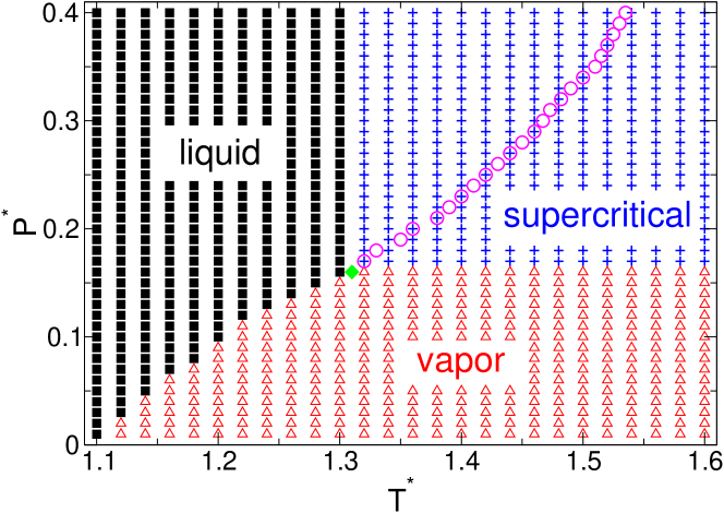
Figure 1: (Color online) Pressure-temperature ($P^{*}-T^{*}$) phase diagram of the liquid, vapor and supercritical fluid phases. The liquid and vapor phases are denoted by black squares and red triangles, respectively. The supercritical fluid phase is denoted by blue crosses. The liquid-vapor critical point estimated from our simulation results and Ref. Smit (1992) is denoted by a green diamond. The approximate location of the liquid-vapor critical point in the $P^{*}-T^{*}$ diagram is $T_{\textrm{c}}^{*}\simeq 1.305$ and $P_{\textrm{c}}^{*}\simeq 0.16$. Circles represent the Widom line emanating from the liquid-vapor critical point. The Widom line is the locus of isobaric specific heat maxima $c_{\textrm{p}}$ estimated from Fig. 6. The Widom line is a continuous extension of the liquid-vapor phase boundary. All points here represent phase points we simulated.

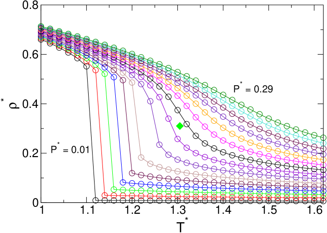
Figure 2: (Color online) Isobaric trajectories in the density-temperature ($\rho^{*}-T^{*}$) phase diagram from pressure $P^{*}$ = 0.01 up to $P^{*}$ = 0.29 in increments of $\Delta P^{*}$ = 0.02. A green diamond represents the estimated liquid-vapor critical point. Below the critical point, when the system crosses the transition temperature, $\rho^{*}$ shows a discontinuous jump at the transition temperature. Above the critical point, $\rho^{*}$ shows the continuous change over the entire temperature range that we investigated.

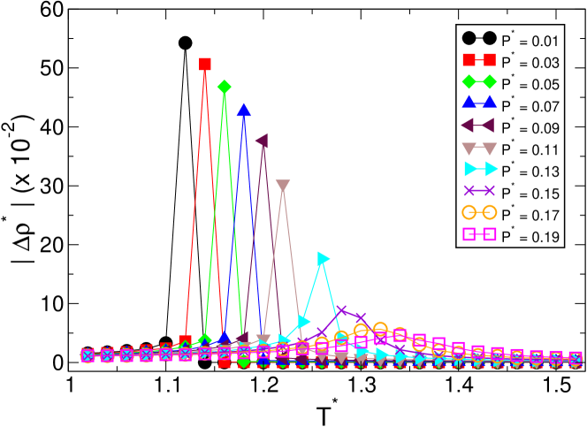
Figure 3: (Color online) The absolute value of the density difference $|\Delta\rho^{*}|$ as a function of temperature $T^{*}$ for different pressures in the subcritical and supercritical regions. The absolute value of the density difference is defined by $|\Delta\rho^{*}(T^{*}_{i})|\equiv|\rho^{*}(T^{*}_{i})-\rho^{*}(T^{*}_{i-1})|$, which is different from the definition of the typical order parameter of the liquid-vapor phase transition $\Delta\rho^{*}\equiv\rho_{\textrm{liquid}}^{*}-\rho_{\textrm{vapor}}^{*}$. The approximate location of the liquid-vapor critical point is $T_{\textrm{c}}^{*}\simeq$ 1.305 and $P_{\textrm{c}}^{*}\simeq$ 0.16. Here we used the temperature step $\Delta T^{*}_{i}\,(=T^{*}_{i}-T^{*}_{i-1})=0.02$.

The $P^{*}-T^{*}$ phase diagram is shown in Figure 1. The first order phase boundary between the liquid and vapor phases terminates at the liquid-vapor critical point ($T^{*}_{\textrm{c}}\simeq$ 1.305 and $P^{*}_{\textrm{c}}\simeq$ 0.16). The Widom line continues the liquid-vapor phase boundary beyond the critical point. In the subcritical region where there is a first order phase transition, the density $\rho^{*}$ along the isobaric path abruptly changes when $T^{*}$ crosses the transition temperature (Fig. 2). However, $\rho^{*}$ in the supercritical region continuously changes as a function of $T^{*}$. These different behaviors of $\rho^{*}$ as a function of $T^{*}$ are clear when we calculate the absolute density difference between two adjacent temperatures $|\Delta\rho^{*}(T^{*}_{i})|\equiv|\rho^{*}(T^{*}_{i})-\rho^{*}(T^{*}_{i-1})|$ (Figs. 3 and 4). Note that this differs from the order parameter of the liquid-vapor phase transition $\Delta\rho\equiv\rho_{\textrm{liquid}}-\rho_{\textrm{vapor}}$. When there is a discontinuous drop in $\rho^{*}(T^{*})$ at the transition temperature in the subcritical region, $|\Delta\rho^{*}|$ shows a spike when $T^{*}$ crosses the same transition temperature. In the supercritical region, as shown in Fig. 4, $|\Delta\rho^{*}|$ shows a maximum at a given temperature, whereas $\rho^{*}$ continuously changes without any abrupt jump.

The maximum in $|\Delta\rho^{*}|$ is associated with a maximum in $d\rho/dT$ that, as we will see later, is associated with the Widom line. Similar behavior has been found in supercooled water. As water is cooled, the density reaches a well known maximum at 4 ^∘C. As the temperature continues to decrease into the supercooled regime, the density decreases until it reaches a minimum as revealed by recent inelastic neutron scattering experiments Liu et al. (2007). With further cooling the density increases in the same way that simple liquids do upon cooling  Debenedetti (2003). Between the density maximum and minimum, there is a maximum in $d\rho/dT$ which coincides with the Widom line of the liquid-liquid transition Liu et al. (2007). Therefore, as we will see later, we expect that the temperature of the maximum in $|\Delta\rho^{*}|$ corresponds to the Widom temperature $T^{*}_{\textrm{w}}$.

To find the Widom line, we calculate the thermal expansion coefficient $\alpha$ defined as Stanley (1971)

$$\alpha = \frac{1}{V}\bigg{(}\frac{\partial V}{\partial T}\bigg{)}_{P}$$ (5)

$$= -\bigg{(}\frac{\partial\ln\rho}{\partial T}\bigg{)}_{P}.$$

Generally, $\alpha$ is associated with fluctuations in the entropy $S$ and volume $V$ Debenedetti (2003),

$$<(\delta S\delta V)>=Vk_{\textrm{B}}T\alpha.$$ (6)

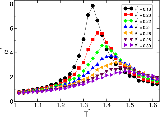
Figure 5: (Color online) Thermal expansion coefficient $\alpha^{*}$ versus temperature $T^{*}$ for different pressures in the supercritical region. As $P^{*}$ increases above the critical pressure $P^{*}_{\textrm{c}}$, the magnitude of the peak in $\alpha^{*}$ decreases. At higher $P^{*}$, the location of the peak moves toward higher $T^{*}$.

In Figure 5, we show $\alpha^{*}$ as a function of $T^{*}$ along the isobaric path in the supercritical region. At low temperature, $\alpha^{*}$ initially increases gradually upon heating, and then starts to increase rapidly upon further heating. As $T^{*}$ increases further, $\alpha^{*}$ finally reaches maximum, and then rapidly decreases. As $P^{*}$ increases above $P^{*}_{\textrm{c}}$ (for $P^{*}>P^{*}_{\textrm{c}}$), the magnitude of the peak in $\alpha^{*}$ decreases, and the temperature of the peak in $\alpha^{*}$ moves toward higher $T^{*}$ as $P^{*}$ increases. $\alpha^{*}$ has the same temperature behavior as $|\Delta\rho^{*}|$ at constant $P^{*}$. In particular, the maximum in $\alpha^{*}$ occurs at the same temperature as that of $|\Delta\rho^{*}|$.

Next, we calculate another thermodynamic response function, the isobaric specific heat $c_{P}$ which is defined as Stanley (1971)

$$c_{P} = \frac{1}{N}\bigg{(}\frac{\partial H}{\partial T}\bigg{)}_{P}$$ (7)

$$= \frac{1}{N}\bigg{(}\frac{\partial(E+PV)}{\partial T}\bigg{)}_{P},$$

where $H$ is the enthalpy and $E$ is the internal energy. Generally, $c_{P}$ is associated with fluctuations in the entropy $S$ Debenedetti (2003),

$$<(\delta S)^{2}>=Nk_{\textrm{B}}c_{P}.$$ (8)

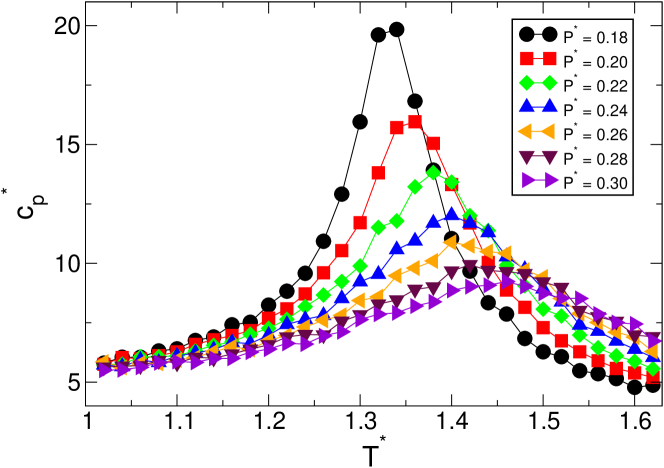
Figure 6: (Color online) Isobaric specific heat $c^{*}_{P}$ versus temperature $T^{*}$ for different pressures in the supercritical region. As $P^{*}$ increases above $P^{*}_{\textrm{c}}$, the magnitude of the peak in $c^{*}_{P}$ decreases. At higher $P^{*}$, the location of the peak moves toward higher $T^{*}$. The behavior of $c^{*}_{P}$ is the same as that of $|\Delta\rho^{*}|$ and $\alpha^{*}$ (see Figs. 4 and 5).

In Figure 6, we show $c^{*}_{P}$ as a function of $T^{*}$ along the isobaric path in the supercritical region. $c^{*}_{P}$ also shows the same temperature behavior that we found for $|\Delta\rho^{*}|$ and $\alpha^{*}$ at constant $P^{*}$ as shown in Figs. 4 and 5. As $P^{*}$ increases from $P^{*}_{\textrm{c}}$ (for $P^{*}>P^{*}_{\textrm{c}}$), the magnitude of the peak in $c^{*}_{P}$ decreases, and the temperature of the peak in $c^{*}_{P}$ moves toward higher $T^{*}$ as $P^{*}$ increases. The temperature of the $c^{*}_{P}$ maximum in Fig. 6 is the Widom temperature $T^{*}_{\textrm{w}}$ at a given pressure Xu et al. (2005); Kumar et al. (2006, 2007, 2008); Stokely et al. (2010). Note that of all the various response functions, the isobaric specific heat is usually used to define the location of the Widom line Xu et al. (2005); Kumar et al. (2006). Based on our calculation of $c^{*}_{P}$, we plot the estimated locations of $c^{*}_{P}$ maxima (the Widom line) in Fig. 1, denoted by open circles.

Next we investigate the standard deviation of an observable $X$ defined as

$$\Sigma_{X}\equiv\sqrt{\big{<}(X-\bar{X})^{2}\big{>}},$$ (9)

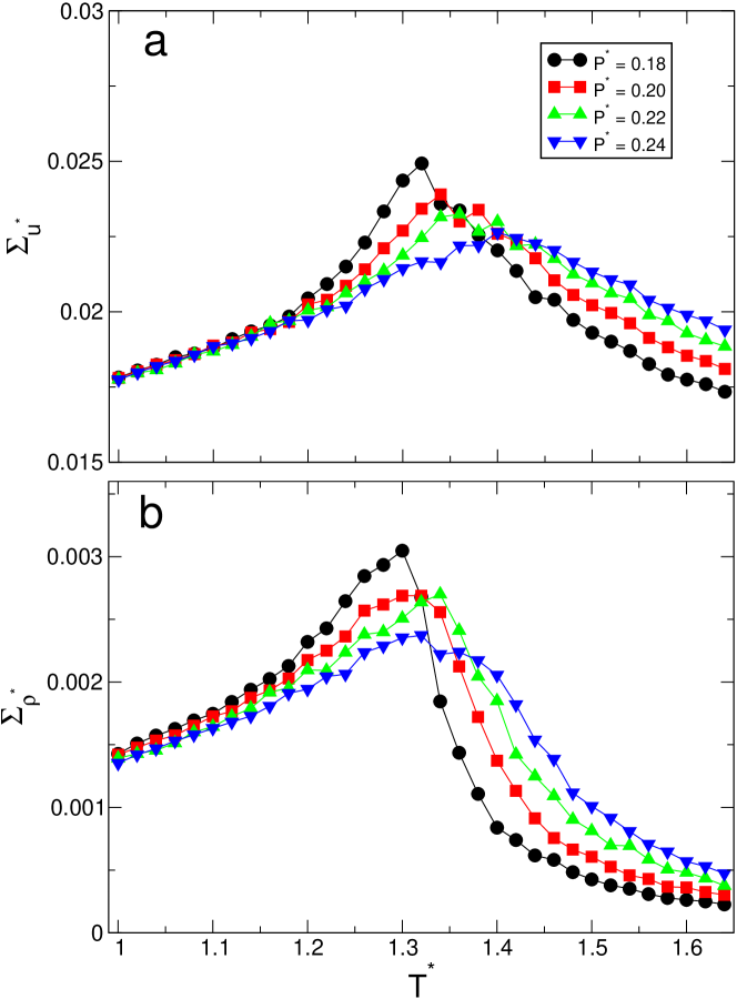
Figure 7: (Color online) Standard deviations (a) $\Sigma_{u^{*}}$ of the potential energy $u^{*}$ per particle and (b) $\Sigma_{\rho^{*}}$ of density $\rho^{*}$ as a function of temperature $T^{*}$. Both $\Sigma_{u^{*}}$ and $\Sigma_{\rho^{*}}$ show maxima around the Widom line.

where $\bar{X}$ is the average of $X$. We calculate the standard deviations $\Sigma_{u^{*}}$ and $\Sigma_{\rho^{*}}$ of the potential energy per particle $u^{*}$ and density $\rho^{*}$, respectively. In Figure 7, we present $\Sigma_{u^{*}}$ and $\Sigma_{\rho^{*}}$ as a function of $T^{*}$. The fluctuations in $u^{*}$ and $\rho^{*}$ rapidly increase as $T^{*}$ approaches $T^{*}_{\textrm{w}}$ from below at fixed $P^{*}$, and they reach their maximum around $T^{*}\simeq T^{*}_{\textrm{w}}$. After crossing $T^{*}_{\textrm{w}}$, $\Sigma_{u^{*}}$ and $\Sigma_{\rho^{*}}$ rapidly decrease as shown in Fig. 7. The location in the phase diagram of the maxima in the variances agrees well with the location of the maxima of the thermodynamic response functions along the Widom line. This is consistent with Eqs. (6) and (8) which relate fluctuations to thermodynamic response functions.

IV Noise Power Spectral Analysis

Let us set up our notation and define what we mean by noise. Let $m(t)$ be a quantity that fluctuates in time. Let $\delta m(t)$ be the deviation from its average value of some quantity $m$ at time $t$. If the processes producing the fluctuations are stationary in time, i.e., translationally invariant in time, then the autocorrelation function of the fluctuations $\langle\delta m(t_{2})\delta m(t_{1})\rangle$ will be a function $\psi(t_{2}-t_{1})$ of the time difference. In this case the Wiener–Khintchine theorem can be used to relate the noise spectral density $S_{m}(\omega)$ to the Fourier transform $\psi(\omega)$ of the autocorrelation function Kogan (1996): $S_{m}(\omega)=2\psi_{m}(\omega)$ where $\omega$ is the angular frequency. In practice $S_{m}(\omega)$ typically is calculated by multiplying the time series $\delta m(t)$ by a windowing or envelope function so that the time series goes smoothly to zero, Fourier transforming the result, taking the modulus squared, and multiplying by two to obtain the noise power Press et al. (1992). (We find that our results are not sensitive to the choice of windowing function, so we do not use a windowing function; this is equivalent to a rectangular window.)

$1/f$ noise, where $\displaystyle f\,\big{(}=\frac{\omega}{2\pi}\big{)}$ is frequency, corresponds to $S_{m}(\omega)\sim 1/\omega$. It dominates at low frequencies and has been observed in a wide variety of systems, such as granular systems, molecular liquids, ionic liquids, a lattice gas model, and resistors Dutta and Horn (1981); Bak et al. (1987); Weissman (1988); Jensen (1990); Sasai et al. (1990); Milotti (1995); Reichhardt and OlsonReichhardt (2003); Mudi et al. (2005); Sharma et al. (2006); Reichhardt and OlsonReichhardt (2007); Chen and Yu (2007); Jeong et al. (2008). For example, long time fluctuations of the potential energy in water and silica exhibiting $1/f$ spectra have been reported in computer simulation studies Sasai et al. (1990); Mudi et al. (2005); Sharma et al. (2006). The $1/f$ power spectrum of the potential energy fluctuations for water is related to the non-exponential relaxation of slow hydrogen bond dynamics Han et al. (2009); Mudi et al. (2005). A study of solvation dynamics in an ionic liquid at room temperature has also shown $1/f$ spectral behavior Jeong et al. (2008). Fluctuations in the number of defects in a disordered two-dimensional liquid also exhibit a $1/f$ power spectrum at low temperatures, suggesting that the dynamics of the system is heterogeneous Reichhardt and OlsonReichhardt (2003, 2007). In addition to the relation between $1/f$ spectral behavior and dynamics, the power spectra can be used as a probe of phase transitions. It has been shown that at a phase transition in classical spin systems (such as the Ising model and Potts model), the low frequency noise of the energy and magnetization fluctuations has a maximum at the transition temperature Chen and Yu (2007).

A simple way to obtain 1/f noise was given by Dutta and Horn Dutta and Horn (1981). We can use the relaxation time approximation to write the equation of motion for $\delta p$:

$$\frac{d\delta p}{dt}=-\frac{\delta p}{\tau}$$ (10)

where $\tau^{-1}$ is the relaxation rate. The autocorrelation function $\psi_{p}(t)$ is given by

$$\psi_{p}(t)=\langle\delta p(t)\delta p(t=0)\rangle.$$ (11)

The Fourier transform is a Lorentzian if there is just one value of $\tau$.

$$S_{p}(\omega)=\frac{A\tau}{1+\omega^{2}\tau^{2}}$$ (12)

where $A$ is an overall scale factor. If there is a broad distribution $g(\tau)$ of relaxation times, then the Fourier transform is a sum of Lorentzians:

$$S_{p}(\omega)=A\int^{\tau_{2}}_{\tau_{1}}\frac{\tau}{1+\omega^{2}\tau^{2}}g(\tau)d\tau$$ (13)

where $\tau_{2}$ and $\tau_{1}$ are the upper and lower limits of the distribution $g(\tau)$ and, hence, of the integral over $\tau$. If we assume that $g(\tau)\sim\tau^{-1}$ Dutta and Horn (1981), then we obtain

$$S_{p}(\omega)\propto\frac{A}{\omega}\bigg{[}\arctan\bigg{(}\frac{1}{\omega\tau_{2}}\bigg{)}-\arctan\bigg{(}\frac{1}{\omega\tau_{1}}\bigg{)}\bigg{]}.$$ (14)

In the low frequency limit ($f\ll\tau_{2}^{-1}\ll\tau_{1}^{-1}$), the power spectrum shows $1/f^{0}$ behavior, and in the high frequency limit ($f\gg\tau_{1}^{-1}\gg\tau_{2}^{-1}$), it shows $1/f^{2}$ behavior. In the intermediate frequency region ($\tau_{2}^{-1}\ll f\ll\tau_{1}^{-1}$), the power spectrum exhibits $1/f$ behavior Dutta and Horn (1981).

Here we use the noise power spectra of $\rho^{*}$ and $u^{*}$ as a probe of the Widom line. The power spectrum of an observable $X(t)$ is defined as

$$S_{X}(f^{*})\equiv\bigg{|}\int X(t^{*})e^{2\pi if^{*}t^{*}}\,dt^{*}\bigg{|}^{2}.$$ (15)

There is no subtraction of the mean $\overline{X}$, so there will be a delta function at $f=0$. $S_{X}(f)$ is otherwise the same as the noise spectrum of the fluctuations $\delta X$.

IV.1 Noise Spectra of Density Fluctuations

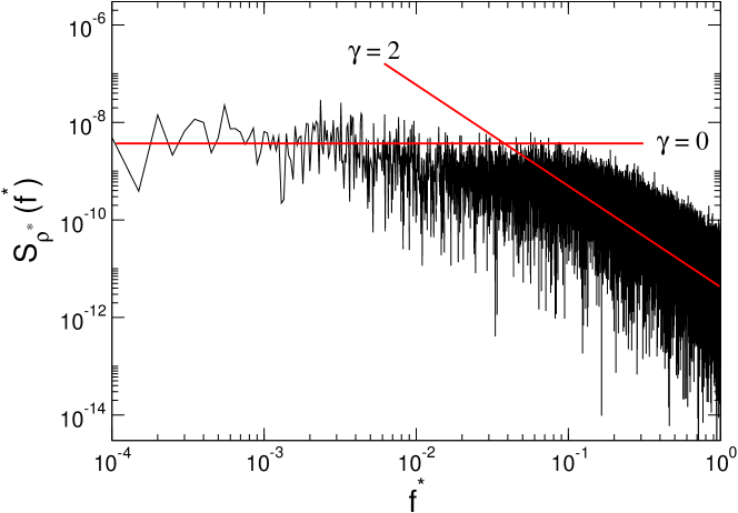
Figure 8: (Color online) Noise power spectrum $S_{\rho^{*}}$ of the density $\rho^{*}$ as a function of frequency $f^{*}$ at $T^{*}$ = 1.02 ($\ll$ $T^{*}_{\textrm{w}}$) and $P^{*}$ = 0.20 in a log-log plot. The two solid lines are fits to $1/f^{*\gamma}$ with the exponents $\gamma$= 0 and 2, respectively.

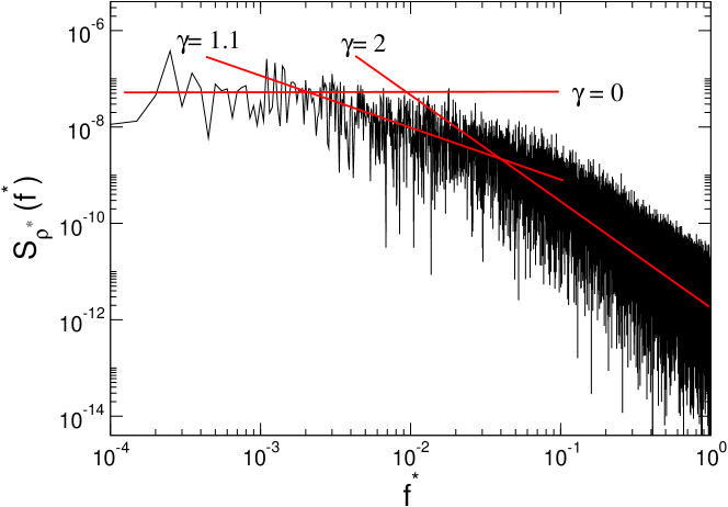
Figure 9: (Color online) The noise power spectrum $S_{\rho^{*}}$ of the density $\rho^{*}$ versus frequency $f^{*}$ at $T^{*}$ = 1.26 ($<$ $T^{*}_{\textrm{w}}$) and $P^{*}$ = 0.20 on a log-log plot. The point ($T^{*}$ = 1.26, $P^{*}$ = 0.20) is located in the liquid region of the phase diagram where the response functions ($\alpha$ and $c_{P}$) change rapidly below $T_{\textrm{w}}$. That is, $\alpha$ and $c_{P}$ at $T^{*}$ = 1.26 rapidly increase as $T^{*}$ increases, as shown in Figs. 5 and 6. The three solid lines are fits to $1/f^{*\gamma}$ with the exponents $\gamma$= 0, 1.1, and 2.

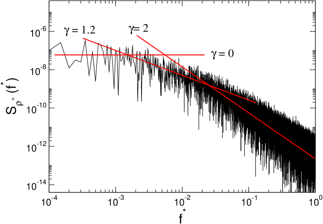
Figure 10: (Color online) Power spectrum $S_{\rho^{*}}$ of the density $\rho^{*}$ as a function of frequency $f^{*}$ at $T^{*}$ = 1.36 ($\approx$ $T^{*}_{\textrm{w}}$) and $P^{*}$ = 0.20 on a log-log scale. The three solid lines indicate fits to $1/f^{*\gamma}$ with the exponents $\gamma$= 0, 1.2, and 2, respectively.

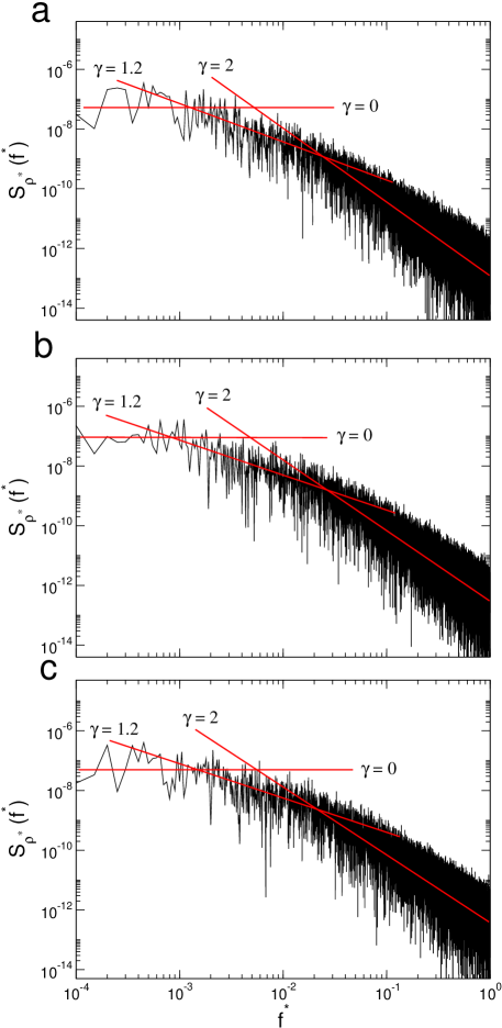
Figure 11: (Color online) Shown on a log-log scale are power spectra $S_{\rho^{*}}$ of the density $\rho^{*}$ as a function of frequency $f^{*}$ at (a) $T^{*}$= 1.34 and $P^{*}$= 0.18, (b) $T^{*}$= 1.38 and $P^{*}$= 0.22, and (c) $T^{*}$= 1.40 and $P^{*}$= 0.24. These temperatures are the Widom temperature $T^{*}_{\textrm{w}}(P^{*})$ at a given pressure $P^{*}$. $S_{\rho^{*}}$ along the Widom line exhibits three distinct frequency regimes where $1/f^{\gamma}$ has exponents $\gamma$= 0, 1.2 and 2.

In Figures 8 to 13, we present the power spectra $S_{\rho^{*}}$ of the density fluctuations as a function of frequency $f^{*}$ for different temperatures along the isobaric path of $P^{*}$= 0.20. When the temperature $T^{*}$ (= 1.02) is far below the Widom temperature $T^{*}_{\textrm{w}}\simeq 1.36$ such that $T^{*}\ll T^{*}_{\textrm{w}}$, $S_{\rho^{*}}$ shows two different frequency dependences: almost flat ($\sim 1/f^{*0}$) at low frequencies and rapidly decreasing ($\sim 1/f^{*2}$) at high frequencies (see Fig. 8). At $T^{*}=1.26$, the thermodynamic response functions start to change rapidly, and $S_{\rho^{*}}(f^{*})$ clearly exhibits three different frequency dependences: flat ($\sim 1/f^{*0}$) at low frequencies, relatively slow decreasing ($\sim 1/f^{*1.1}$) with increasing frequency at intermediate frequencies, and rapidly decreasing ($\sim 1/f^{*2}$) at high frequencies (see Fig. 9). On the Widom line ($T^{*}=1.36\simeq T^{*}_{\textrm{w}}$), $S_{\rho^{*}}$, as shown in Fig. 10, shows the same three different frequency dependences as in Fig. 9: flat ($\sim 1/f^{*0}$) at low frequencies, relatively slow decreasing ($\sim 1/f^{*1.2}$) at intermediate frequencies and rapidly decreasing ($\sim 1/f^{*2}$) at high frequencies. For different $P^{*}$, $S_{\rho^{*}}(f)\sim 1/f^{*\gamma}$ at the corresponding Widom temperature $T^{*}_{\textrm{w}}(P^{*})$ with $\gamma$= 0, 1.2 and 2, respectively (see Fig. 11). Interestingly, in the intermediate frequency region, $\gamma\simeq 1.2$ all along the Widom line, independent of $P^{*}$.

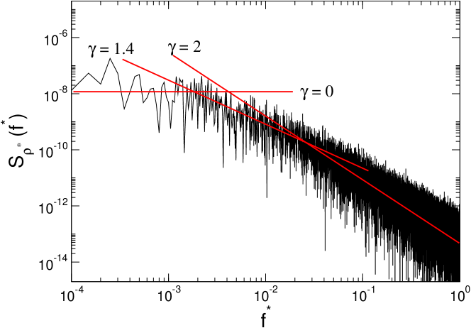
Figure 12: (Color online) The power spectrum $S_{\rho^{*}}$ of the density $\rho^{*}$ as a function of frequency $f^{*}$ at $T^{*}$ = 1.44 ($>$ $T_{\textrm{w}}$) and $P^{*}$ = 0.20 on a log-log scale. $T^{*}$ = 1.44 is located in the region of the phase diagram where the response functions ($\alpha$ and $c_{P}$) change rapidly above $T_{\textrm{w}}$. That is, $\alpha$ and $c_{P}$ at $T^{*}$ = 1.44 rapidly decrease as $T^{*}$ increases, as shown in Figs. 5 and 6. The three solid lines are fits to $1/f^{*\gamma}$ with the exponents $\gamma$ = 0, 1.4 and 2, respectively.

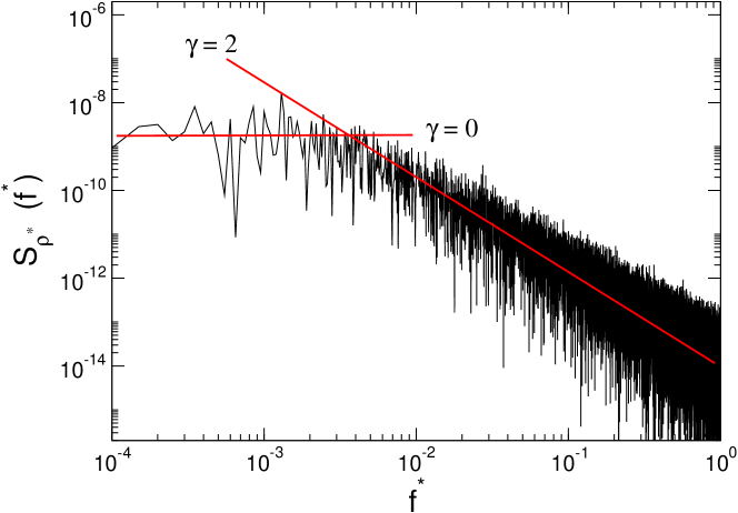
Figure 13: (Color online) Shown on a log-log plot is the power spectrum $S_{\rho^{*}}$ of the density $\rho^{*}$ as a function of frequency $f^{*}$ at $T^{*}$ = 1.58 $(\gg T^{*}_{\textrm{w}})$ and $P^{*}=0.20$. The two solid lines are fits to $1/f^{*\gamma}$ with the exponents $\gamma$= 0 and 2, respectively.

The behavior of $S_{\rho^{*}}$ at temperatures in the vicinity of $T^{*}_{\textrm{w}}$ is similar to that seen along the Widom line. Below but close to $T^{*}_{\textrm{w}}$ where the thermodynamic response functions still change rapidly (as in the case of $T^{*}$ = 1.44 shown in Fig. 12), $S_{\rho^{*}}$ shows three different frequency dependences: white ($\sim 1/f^{*0}$) at low frequencies, relatively slow decreasing ($\sim 1/f^{*1.4}$) at intermediate frequencies and rapidly decreasing ($\sim 1/f^{*2}$) at high frequencies. When $T^{*}$ is far away from $T^{*}_{\textrm{w}}$, there are two frequency dependences: flat ($\sim 1/f^{*0}$) at low frequencies and rapidly decreasing ($\sim 1/f^{*2}$) at high frequencies (see Fig. 13 where $T^{*}=1.58\gg T^{*}_{\textrm{w}}$)).

When $T^{*}$ is far away from $T^{*}_{\textrm{w}}$, the density fluctuations relax exponentially with a single relaxation time. As explained in the simple model of $1/f$ noise in Eqs. (12) and (14), $1/f$ spectral behavior can be connected with a broad distribution of relaxation times. Therefore, our results imply that as $T^{*}$ approaches $T^{*}_{\textrm{w}}$, the density fluctuations are becoming more complicated and are relaxing with a broad distribution of relaxation times. The appearance of the $1/f$ spectral behavior near the Widom line in a narrow frequency range might be from the fact that the Widom line of the liquid-vapor transition is located at very high temperatures, at which heterogeneous dynamics generally does not occur Reichhardt and OlsonReichhardt (2003, 2007), so that the distribution of relaxation times might have a narrow range of the values as implied by Eq. (14). Note that $S_{\rho^{*}}$ along the Widom line does not provide a clear distinction between liquid-like and vapor-like behaviors as the recent x-ray scattering experiments on the velocity of sound in argon did Simeoni et al. (2010).

IV.2 Noise Spectra of Potential Energy Fluctuations

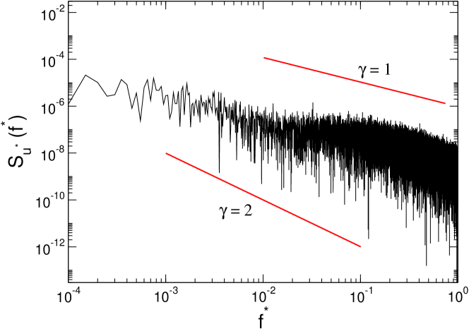
Figure 14: (Color online) The power spectrum $S_{u^{*}}$ of the potential energy per particle $u^{*}$ as a function of frequency $f^{*}$ at $T^{*}$ = 1.34 $(\simeq T^{*}_{\textrm{w}})$ and $P^{*}$ = 0.20 on a log-log scale. The two solid lines are guides to the eye and indicate $1/f^{*\gamma}$ with the exponents $\gamma$= 1 and 2, respectively.

We now examine the fluctuations in the potential energy $u^{*}$ per particle. In contrast to $S_{\rho^{*}}$, the noise spectra $S_{u^{*}}$ of potential energy fluctuations does not clearly show three different frequency dependences on the Widom line, as shown in Fig. 14. $S_{u^{*}}(f)$ is white at low frequencies and then slowly decreases with increasing frequency. Previous simulations of argon at $T$ = 95 K found that the noise spectrum of the total potential energy fluctuations is white over a wide range of frequencies, followed by a rapid decrease at high frequencies Sasai et al. (1990). Interestingly, as opposed to the total potential energy, the potential energy fluctuations of an individual argon atom exhibit $1/f$ noise in an intermediate frequency range ($1\lesssim f\lesssim 10$ cm^-1) Sasai et al. (1990). The potential energy of an argon cluster also exhibits $1/f$ noise in an intermediate frequency range ($f\lesssim 1$ cm^-1), indicating that locally the system can have a distribution of relaxation times, e.g., at the core and surface of the argon cluster Sasai et al. (1990). The origin of the difference between the total potential energy fluctuations of simple liquids and the potential energy fluctuations individual atoms and clusters remains elusive Sasai et al. (1990). An investigation of this difference would be interesting, but is beyond the scope of the present work. We should also mention that a previous computational study found that the long-time total potential energy fluctuations of water does exhibit $1/f$ noise, unlike simple liquids like argon Sasai et al. (1990). Water has a random hydrogen-bond network that has non-exponential relaxation processes, whereas simple liquids do not have such structures Han et al. (2009); Matsumoto and Ohmine (1996).

IV.3 Block Average of Variances in Density and Potential Energy

We are able to estimate the correlation time of an observable $X(t)$ by calculating the block average Frenkel and Smit (2002); Chen and Yu (2007); Rapaport (2004); Flyvbjerg and Petersen (1989); Ferrenberg et al. (1991); Yu and Carruzzo (2004). To calculate the block average, we take a time series of $X(t)$, divide the time series into blocks or bins of equal size, calculate the thermodynamic quantity such as the variance $\Sigma_{X}$ of $X$ for each bin, and then average over all the bins to obtain the block average. If the quantity is not a linear function of $X$, then the block average can depend on the bin size. So one can use the same time series over again to calculate the block average with a different bin size, and see if the block average changes with bin size. Typically, the block average will increase with bin size before saturating at a constant value corresponding to the equilibrium value of the quantity Chen and Yu (2007); Yu and Carruzzo (2004). The saturation occurs when the bin size exceeds the correlation time Rapaport (2004); Flyvbjerg and Petersen (1989); Ferrenberg et al. (1991).

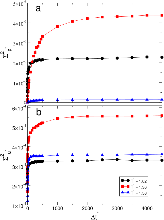
Figure 15: (Color online) Block averages of (a) the density variance $\Sigma^{2}_{\rho^{*}}$, and (b) the potential energy variance $\Sigma^{2}_{u^{2}}$ as a function of the block size $\Delta t^{*}$ at $P^{*}$ = 0.20 for different temperatures $T^{*}$ = 1.02 ($<T^{*}_{\textrm{w}}$), 1.36 ($\simeq T^{*}_{\textrm{w}}$), and 1.58 ($>T^{*}_{\textrm{w}}$).

In Figure 15, we calculate the block average of the variance in the density ($\Sigma^{2}_{\rho^{*}}$) and in the potential energy per particle ($\Sigma^{2}_{u^{*}}$) as a function of the block size ($\Delta t^{*}$) for different temperatures. By comparing the block averages for three different temperatures, we find that the correlation times of both $\rho^{*}$ and $u^{*}$ are largest at the Widom temperature ($T^{*}_{\textrm{w}}\simeq 1.36$), where $|\Delta\rho^{*}|$ and the specific heat have their maxima. The block averages for both quantities saturate at a constant value at approximately $\Delta t^{*}\sim 10^{3}$. This block size indicates the largest correlation time and corresponds to the crossover frequency between the $1/f^{*0}$ and $1/f^{*}$ spectral behaviors that occurs at approximately $f^{*}\sim 10^{-3}$. Recent Monte Carlo studies of the classical spin systems also found that the crossover between white noise at low frequencies and $1/f$ noise at higher frequencies occurred at a frequency corresponding to the inverse of the largest correlation time Chen and Yu (2007). It is interesting to note that at the Widom temperature, the correlation time of the density fluctuations is larger than that of the potential energy fluctuations.

IV.4 Maximum of Low Frequency Noise as a Signature of the Widom Line

A maximum in the low frequency white noise can be a signature of a phase transition or a crossover. For example, Monte Carlo simulations have found that the low frequency white noise in the energy and magnetization is a maximum at the phase transition of the 2D ferromagnetic Ising model and the 2D 5-state Potts model Chen and Yu (2007). In addition, the maximum in the noise power of the defect density at low frequency occurs at the onset of defect proliferation in a two-dimensional liquid modeled by a Yukawa potential Reichhardt and OlsonReichhardt (2003, 2007).

We have found that the low frequency white noise in the density and the potential energy is a maximum at the Widom line. In Figure 16, we show values of the power spectra at low frequency. We take the average value of the white noise part of the power spectrum $S_{X}$ where $X$ is $\rho^{*}$ or $u^{*}$ at each $T^{*}$. Each $S_{X}(T^{*})$ value in Fig. 16 is normalized by $S_{X}(T^{*}_{0}=1)$ to obtain the ratio $S_{X}(T^{*})/S_{X}(T^{*}_{0}=1)$. For both the density ($X=\rho^{*}$) and potential energy ($X=u^{*}$) fluctuations, $S_{X}(T^{*})/S_{X}(T^{*}_{0}=1)$ has a maximum in the vicinity of the Widom temperature $T^{*}_{\textrm{w}}$. Therefore, our results show that a maximum in the low frequency power can provide an additional signature of the Widom line.

V Discussion and Summary

We have performed molecular dynamics simulations of a Lennard-Jones fluid in the supercritical region of the phase diagram to probe the Widom line of the liquid-vapor phase transition and its effect on the power spectra of the density and potential energy fluctuations.

Extending from the liquid-vapor critical point, the Widom line, the locus of the maxima of the thermodynamic response functions, is a continuation of the liquid-vapor phase transition line. The thermodynamic response functions in the supercritical region, such as the thermal expansion coefficient and the isobaric specific heat, have maxima along the Widom line. Similar results have been found by studies of the Widom line of the hypothesized liquid-liquid phase transition in supercooled water Xu et al. (2005); Kumar et al. (2006, 2007, 2008); Stokely et al. (2010); Abascal and Vega (2010); Wikfeldt et al. (2011).

We studied the power spectra of the density and potential energy fluctuations in the supercritical region. Far away from the Widom line, the noise in the density fluctuations is white at low frequencies and goes as $1/f^{2}$ at higher frequencies. $1/f^{2}$ behavior is consistent with an exponential relaxation process characterized by a single relaxation time. In the vicinity of the Widom line we found that the density noise spectrum could be divided into 3 frequency regimes: $1/f^{0}$ at low frequency, $1/f^{1.2}$ at intermediate frequencies, and $1/f^{2}$ at high frequencies. The intermediate region $1/f$ noise implies that there is a distribution of relaxation times associated with the maxima in the response functions along the Widom line. Eq. (14) implies that the narrowness of the frequency range where there is $1/f$ noise is due to a narrow distribution of relaxation times. The narrow width of the intermediate region might be due to the fact that density correlations are short lived at high temperatures. In contrast to the density fluctuations, the power spectrum of the potential energy fluctuations along the Widom line does not exhibit three distinct frequency regimes. Finally, we found that the low frequency white noise of the density and potential energy fluctuations have their maxima along the Widom line. This suggests that noise power spectra, which have been used to probe phase transitions Chen and Yu (2007), can also be used to locate the Widom line.

Figure 4: (Color online) Absolute value of the density difference $|\Delta\rho^{*}|$ versus temperature $T^{*}$ for different pressures in the supercritical region. The magnitude of the peaks decreases as the system moves away from the liquid-vapor critical point. At higher $P^{*}$, the location of the peak moves toward higher $T^{*}$.

Figure 16: (Color online) The magnitude of the normalized power spectra $S_{X}(T^{*})/S_{X}(T^{*}_{0}=1)$ versus temperature $T^{*}$ for the density ($X=\rho^{*}$) and potential energy per particle ($X=u^{*}$) at low frequency at $P^{*}$ = 0.2. Both $S_{\rho^{*}}(T^{*})/S_{\rho^{*}}(T^{*}_{0}=1)$ and $S_{u^{*}}(T^{*})/S_{u^{*}}(T^{*}_{0}=1)$ exhibit maxima in the vicinity of the Widom line.