Exact results for the spectra of interacting bosons and fermions
on the lowest Landau level

Abstract

A system of $N$ interacting bosons or fermions in a two-dimensional harmonic potential (or, equivalently, magnetic field) whose states are projected onto the lowest Landau level is considered. Generic expressions are derived for matrix elements of any interaction, in the basis of angular momentum eigenstates. For the fermion “ground state” ($N=1$ Laughlin state), this makes it possible to exactly calculate its energy all the way up to the mesoscopic regime $N\sim 1000$. It is also shown that for $N=3$ and Coulomb interaction, several rational low-lying values of energy exist, for bosons and fermions alike.

I Introduction

This paper is a sequel of Ref. LLL , where exact eigenstates were discussed for bosons with contact interaction in the lowest Landau level (LLL) of a strong magnetic field in two dimensions, as well as eigenenergies for fermions with Laplacian delta interaction, for which Laughlin wavefunctions are known to be exact eigenstates. In this paper, general expressions for matrix elements of an arbitrary central interaction — a sum of two body-interactions $V(r_{ij})$ whose Fourier transform admits a Laurent expansion $v(k)={a_{-1}\over k}+a_{0}+a_{1}k+\ldots$ — projected onto the lowest Landau level are derived. These include $1/r^{n}$ with any $n$, as well as contact (delta) and Laplacian delta interactions. An exact expression of the interaction energy $E(N)$ for the $N$-fermion “ground state” (the $n=1$ Laughlin state, which is actually the ground state in the presence of a harmonic potential) is derived from which the large $N$ asymptotic behavior can be obtained. For Coulomb interactions, the asymptotics is $E(N)\propto N^{3/2}$, which is confirmed by direct numerical calculation up to $N=1000$. Also for Coulomb interactions, in the three-body problem, rational values of energy exist for low values of the total angular momentum, for bosons and fermions alike.

Clearly, on the experimental side, we have in mind rotating Bose-Einstein condensates BEC on the one hand, and strongly correlated Quantum Hall fermion droplets QHFD on the other hand. In both cases a magnetic field is present, be it real in the quantum Hall case, or effective (due to the rotation of the condensate) in the BEC case. In the sequel, as a matter of simplification, we consider a harmonic trap one-body Hamiltonian, and the projection of the interaction is made on the one-body harmonic eigenstates

$$\langle z,\bar{z}|0,l\rangle=\left({{\omega^{l+1}\over\pi l!}}\right)^{{1\over 2}}z^{l}\mathrm{e}^{-{1\over 2}\omega z\bar{z}}\;,$$ (1)

Indeed, if a magnetic field were added to the harmonic trap, the one-body eigenstates corresponding to the LLL (Landau level number $n=0$, angular momentum $l\geq 0$) would be the LLL-harmonic eigenstates basis (in complex coordinates)

$$\langle z,\bar{z}|0,l\rangle=\left({{\omega_{\mathrm{t}}^{l+1}\over\pi l!}}\right)^{{1\over 2}}z^{l}\mathrm{e}^{-{1\over 2}\omega_{\mathrm{t}}z\bar{z}}\to_{\omega_{\mathrm{c}}\to 0}\left({{\omega^{l+1}\over\pi l!}}\right)^{{1\over 2}}z^{l}\mathrm{e}^{-{1\over 2}\omega z\bar{z}}\;,$$ (2)

where $\omega_{\mathrm{t}}=\sqrt{\omega_{\mathrm{c}}^{2}+\omega^{2}}$, $\omega_{\mathrm{c}}$ being half the cyclotron frequency. Note that since we diagonalize the system in a given angular momentum sector (the angular momentum operator commutes with the interaction Hamiltonian), the magnetic field simply shifts the total energy by a constant term, which is therefore ignored here.

II MATRIX ELEMENTS

The Hamiltonian for $N$ interacting particles in a harmonic trap is

$${\cal{H}}=-2\sum_{i=1}^{N}\partial_{i}\bar{\partial}_{i}+\frac{\omega^{2}}{2}\sum_{i=1}^{N}z_{i}\bar{z}_{i}+\sum_{i<j=1}^{N}V(|z_{i}-z_{j}|)\;.$$ (3)

As long as the interaction potential $V(|z_{i}-z_{j}|)$ vanishes at infinity, so that the harmonic potential dominates, the asymptotics of the wave function can be detached as usually,

$$\psi(z_{1},\bar{z}_{1},...,z_{N},\bar{z}_{N})=\exp\left(-\frac{\omega}{2}\sum_{i=1}^{N}z_{i}\bar{z}_{i}\right)\chi(z_{1},\bar{z}_{1},...,z_{N},\bar{z}_{N})\;;$$ (4)

then the Hamiltonian acting on $\chi$ is

$$H=H_{0}+\sum_{i<j=1}^{N}V(|z_{i}-z_{j}|)$$ (5)

where the free Hamiltonian $H_{0}$ is

$$H_{0}=\sum_{i=1}^{N}(-2\partial_{i}\bar{\partial}_{i}+\omega+\omega z_{i}\partial_{i}+\omega\bar{z}_{i}\bar{\partial}_{i})\;.$$ (6)

From now on one sets $\omega=1$. The LLL projector has the form

$$P\chi=\prod_{i=1}^{N}\left[\frac{1}{\pi}\int\mathrm{e}^{-z^{\prime}_{i}\bar{z}^{\prime}_{i}+z_{i}\bar{z}^{\prime}_{i}}\mathrm{d}z^{\prime}_{i}\mathrm{d}\bar{z}^{\prime}_{i}\right]\chi(z^{\prime}_{1},\bar{z}^{\prime}_{1},...,z^{\prime}_{N},\bar{z}^{\prime}_{N})\;.$$ (7)

LLL functions are analytic

$$\chi=\chi(z_{1},...,z_{N})\;;$$ (8)

for such a function, $P\chi=\chi$, and, since $\chi$ does not depend on $\bar{z}$’s,

$$PH_{0}\chi=\omega(N+\sum_{i=1}^{N}z_{i}\partial_{i})\chi\;.$$ (9)

Perform a Fourier transform of the interaction,

$$V(r)=\int\frac{\mathrm{d}^{2}{\vec{k}}}{2\pi}\mathrm{e}^{\displaystyle\mathrm{i}{\vec{k}\vec{r}}}v(k)\;.$$ (10)

and introduce the complex coordinates

$${\vec{k}\vec{r}}=\frac{{\bf\bar{k}}z}{2}+\frac{{\bf k}\bar{z}}{2},\quad{\bf k}=k_{x}+\mathrm{i}k_{y}\;.$$ (11)

One finally obtains the LLL-projected interaction

$$P\sum_{i<j=1}^{N}V(|z_{i}-z_{j}|)\chi = \sum_{i<j=1}^{N}\int\exp\left[\mathrm{i}\frac{\bar{\bf k}(z_{i}-z_{j})}{2}\right]\frac{v(k)}{2\pi}\,\chi(...\,,z_{i}+\mathrm{i}\frac{{\bf k}}{2},...\,,z_{j}-\mathrm{i}\frac{{\bf k}}{2},...)\,\mathrm{e}^{-\frac{k^{2}}{2}}\mathrm{d}{\bf k}\,\mathrm{d}{\bf{\bar{k}}}$$ (12)

$$= \sum_{i<j=1}^{N}\sum_{n_{1},n_{2}=0}^{\infty}\int_{0}^{\infty}k^{2(n_{1}+n_{2})+1}v(k)\mathrm{e}^{-\frac{k^{2}}{2}}\mathrm{d}k\frac{(-1)^{n_{1}}(z_{i}-z_{j})^{n_{1}+n_{2}}}{n_{1}!\,n_{2}!\,(n_{1}+n_{2})!\,2^{2(n_{1}+n_{2})}}\frac{\partial^{n_{1}+n_{2}}}{\partial z_{i}^{n_{1}}\partial z_{j}^{n_{2}}}\chi(z_{1},...,z_{N})$$

$$= \sum_{i<j=1}^{N}\sum_{n=0}^{\infty}\int_{0}^{\infty}k^{2n+1}v(k)\mathrm{e}^{-\frac{k^{2}}{2}}\mathrm{d}k\frac{(z_{i}-z_{j})^{n}(\partial_{j}-\partial_{i})^{n}}{(n!)^{2}\,2^{2n}}\chi(z_{1},...,z_{N})\;,$$

where one has expanded every term containing the $z$’s into Taylor series, substituted ${\bf k}=k\exp(\mathrm{i}\phi)$, and integrated over $\phi$.

In the last expression of (12) the expansion coefficient $\int_{0}^{\infty}k^{2n+1}v(k)\mathrm{e}^{-\frac{k^{2}}{2}}\mathrm{d}k$ is well defined as long as $v(k)$ admits a Laurent expansion $v(k)=\sum_{m=-1}^{\infty}a_{m}k^{m}$ such that

$$\int_{0}^{\infty}k^{2n+1}k^{m}\mathrm{e}^{-\frac{k^{2}}{2}}\mathrm{d}k=2^{n+{m\over 2}}\Gamma(n+1+{m\over 2})$$ (13)

An elementary LLL $N$-body wave function is

$$\chi=\prod_{i=1}^{N}z_{i}^{l_{i}}\;;$$ (14)

for bosons (fermions), it has to be (anti)symmetrized. It is an eigenfunction of the total angular momentum, $L=\sum_{i=1}^{N}l_{i}$, and thus an eigenfunction of $H_{0}$. It is obvious from (12) that $P\sum_{i<j=1}^{N}V(|z_{i}-z_{j}|)$ conserves the angular momentum (as any central interaction should do), therefore it is enough to diagonalize it in each sector of given $L$.

The states with the lowest absolute value of angular momentum — for brevity, we will refer to them as “ground states” (which they are if there is a harmonic potential), both of bosons,

$$\chi_{0}^{\mathrm{B}}(N)=1\;,\quad L=0\;,$$ (15)

and of fermions,

$$\chi_{0}^{\mathrm{F}}(N)=\prod_{i<j=1}^{N}(z_{i}-z_{j})\;,\quad L=\frac{N(N-1)}{2}\;,$$ (16)

are nondegenerate with respect to angular momentum, which implies that they are both eigenfunctions of $P\sum_{i<j=1}^{N}V(|z_{i}-z_{j}|)$. For bosons, this can be seen directly by looking at Eq. (12) where only the $n=0$ term survives so that

$$P\sum_{i<j=1}^{N}V(|z_{i}-z_{j}|)=\frac{N(N-1)}{2}\int v(k)k\,\mathrm{e}^{-\frac{k^{2}}{2}}\mathrm{d}k\;$$ (17)

and thus

$$E(N)=\frac{N(N-1)}{2}\int v(k)k\,\mathrm{e}^{-\frac{k^{2}}{2}}\mathrm{d}k$$

(the diagonal matrix element of the interaction in the momentum representation.)

III Fermion ground state

In the Fermi case it is also possible to solve the eigenvalue equation

$$P\sum_{i<j=1}^{N}V(|z_{i}-z_{j}|)\chi_{0}^{\mathrm{F}}(N)=E(N)\chi_{0}^{\mathrm{F}}(N)\;,$$ (18)

where $P\sum_{i<j=1}^{N}V(|z_{i}-z_{j}|)$ is given in (12).

The key observation is that, since said state $\chi_{0}^{\mathrm{F}}(N)$ is known to be an eigenstate of $P\sum_{i<j=1}^{N}V(|z_{i}-z_{j}|)$ it is not necessary to calculate the whole LHS of (18). Being a Vandermonde determinant $\chi_{0}^{\mathrm{F}}(N)$ rewrites as

$$\chi_{0}^{\mathrm{F}}(N)=\prod_{l=1}^{N}z_{l}^{l-1}+\cdots\;,$$ (19)

where the omitted $(N!-1)$ terms come from antisymmetrization. It follows that the coefficient in front of $\prod_{l=1}^{N}z_{l}^{l-1}$ on the LHS of Eq. (18) is necesseraly $E(N)$. Return to the second line of Eq. (12) and let $\chi(z_{1},...,z_{N})$ be the monomial $\prod_{l=1}^{N}z_{l}^{p_{l}}$. Then a term with given $i$ and $j$ in the sum on the RHS of that equation will be a sum of monomials in each of which only the powers of $z_{i}$ and $z_{j}$ are different from $p_{i}$ and $p_{j}$, respectively (and the power of any $z_{l}$ with $l\neq i,j$ is still $p_{l}$). Moreover, the sum of all powers of $z$’s, which is the total angular momentum, never changes. Hence, there are only two cases when $P\sum_{i<j=1}^{N}V(|z_{i}-z_{j}|)\chi$ can contain $\prod_{l=1}^{N}z_{l}^{l-1}$ as one of its terms: (i) $p_{l}=l-1$; (ii) $p_{l}=l-1$ ($l\neq i,j$); $p_{i}=j-1$; $p_{j}=i-1$ (i.e., $z_{i}$ and $z_{j}$ are interchanged; in the Vandermonde determinant, the corresponding monomial comes with a minus sign). Moreover, in each of these two cases, for given $n_{1}$ and $n_{2}$, no more than a single term in the binomial expansion of $(z_{i}-z_{j})^{n_{1}+n_{2}}$ will yield the desired contribution. In case (i), that term is $z_{i}^{n_{1}}z_{j}^{n_{2}}$ (so that the powers of $z_{1}$ and $z_{2}$ stay unchanged after differentiation followed by multiplication); in case (ii), it is $z_{i}^{n_{1}+i-j}z_{j}^{n_{2}+j-i}$ [so that the power of $z_{i}$, which is $j-1$ in $\chi$, becomes $j-1-n_{1}+n_{1}+i-j=i-1$ in the $P\sum_{i<j=1}^{N}V(|z_{i}-z_{j}|)\chi$; likewise for $z_{j}$]. The maximum possible values of $n_{1}$ and $n_{2}$ are the powers of $z_{i}$ and $z_{j}$, respectively, in $\chi$. Taking this into account and gathering all the coefficients, we obtain

$$E(N)=\int_{0}^{\infty}f(N,k)v(k)k\,\mathrm{e}^{-\frac{k^{2}}{2}}\mathrm{d}k\;,$$ (20)

where

$$f(N,k)=\sum_{i<j=1}^{N}\left[\sum_{n_{1}=0}^{i}\sum_{n_{2}=0}^{j}c_{ijn_{1}n_{2}}(k)-\sum_{n_{1}=0}^{j}\sum_{n_{2}=0}^{i}d_{ijn_{1}n_{2}}(k)\right]$$ (21)

with

$$c_{ijn_{1}n_{2}}(k) = \frac{(-1)^{n_{1}+n_{2}}}{(n_{1}!n_{2}!)^{2}}(i-n_{1})_{n_{1}}(j-n_{2})_{n_{2}}\left(\frac{k}{2}\right)^{2(n_{1}+n_{2})}\;,$$

$$d_{ijn_{1}n_{2}}(k) = \frac{(-1)^{n_{1}+n_{2}+j-i}}{n_{1}!n_{2}!(n_{1}+i-j)!(n_{2}+j-i)!}(j-n_{1})_{n_{1}}(i-n_{2})_{n_{2}}\left(\frac{k}{2}\right)^{2(n_{1}+n_{2})}\;;$$ (22)

$(x)_{n}\equiv\frac{\Gamma(x+n)}{\Gamma(x)}$ is the Pochhammer symbol.

The summation over $n_{1}$ and $n_{2}$ can be performed explicitly, by noting that

$$c_{ijn_{1}n_{2}}(k) = f_{iin_{1}}(k)f_{jjn_{2}}(k)\;,$$

$$d_{ijn_{1}n_{2}}(k) = (-1)^{j-i}f_{ijn_{1}}(k)f_{jin_{2}}(k)\;,$$ (23)

where

$$f_{ijn}(k)=\frac{(-1)^{n}}{n!(n+i-j)!}(j-n)_{n}\left(\frac{k}{2}\right)^{2n}\;,$$ (24)

and that

$$\sum_{n=0}^{j}f_{ijn}(k)=\frac{(j-1)!}{(i-1)!}L_{j-1}^{i-j}\left(\frac{k^{2}}{4}\right)\;.$$ (25)

Hence,

$$f(N,k)=\sum_{i<j=1}^{N}\left[L_{i-1}\left(\frac{k^{2}}{4}\right)L_{j-1}\left(\frac{k^{2}}{4}\right)-(-1)^{j-i}L_{j-1}^{i-j}\left(\frac{k^{2}}{4}\right)L_{i-1}^{j-i}\left(\frac{k^{2}}{4}\right)\right]\;.$$ (26)

For example for the first values of $N$ one has

$$f(2,k) = -\frac{k^{2}}{2}+1\;,$$

$$f(3,k) = -\frac{k^{6}}{64}+\frac{9k^{4}}{32}-\frac{9k^{2}}{4}+3\;,$$

$$f(4,k) = -\frac{k^{10}}{6144}+\frac{25k^{8}}{3072}-\frac{k^{6}}{6}+\frac{23k^{4}}{16}-6k^{2}+6\;.$$ (27)

Substituting into Eq. (20) gives, within the LLL-projection approximation, the energy of the $N$-fermion Vandermonde state $\chi_{0}^{\mathrm{F}}(N)$ for any central pairwise interaction.

Further simplification is possible. A recurrency relation is

$$f(N+1,k)-f(N,k)=L_{N-1}^{1}\left(\frac{k^{2}}{4}\right)L_{N}\left(\frac{k^{2}}{4}\right)+\sum_{i=1}^{N}\left[(-1)^{N-i}L_{N}^{i-N-1}\left(\frac{k^{2}}{4}\right)L_{i-1}^{N+1-i}\left(\frac{k^{2}}{4}\right)\right]\;,$$ (28)

where in the first term, $\sum_{p=0}^{n}L_{p}^{a}(x)=L_{n}^{a+1}(x)$ has been used. This is much more efficient than (26), as it requires to compute a single sum for each subsequent $N$, instead of a double sum.

One wants to find an expression for the chemical potential

$$\mu(N)\equiv E(N+1)-E(N)$$ (29)

Using

$$L_{n}^{a}(x)=\frac{1}{n!}e^{x}x^{-a}\frac{d^{n}}{dx^{n}}\left(e^{-x}x^{n+a}\right)$$ (30)

one rewrites the second sum in Eq. (28) as $\sum_{i=0}^{N}\frac{(k^{2}/4)^{N+1-i}}{i!(N+1)!}U(-i,2-i+N,k^{2}/4)^{2}$, which, taking into account (29), yields

$$\mu(N)=2\int_{0}^{\infty}v(2\sqrt{x})\mathrm{e}^{-2x}\,\left[L_{N}(x)L_{N-1}^{1}(x)-\sum_{i=0}^{N}\frac{x^{N+1-i}}{i!(N+1)!}U(-i,2-i+N,x)^{2}\right]\,\mathrm{d}x\;,$$ (31)

where $U(a,b,x)$ is the confluent hypergeometric function of the second kind.

Note that if $v(k)$ is a power,

$$v(k)=c\,k^{m}\;,$$ (32)

the integration in Eq. (20) can be performed explicitly, using PBM

$$\int_{0}^{\infty}x^{\alpha-1}\mathrm{e}^{-2x}L_{m}^{\gamma}(x)L_{n}^{\lambda}(x)\mathrm{d}x=\frac{(1+\gamma)_{m}\,(1-\alpha+\lambda)_{n}}{m!\,n!}\,\Gamma(\alpha)\,{}_{3}F_{2}(\alpha,\,\alpha-\lambda,\,1+\gamma+m;\,\alpha-\lambda-n,\,1+\gamma;\,-1)\;.$$ (33)

As a result,

$$\mu(N) = c\,2^{m+1}\Gamma(\frac{m}{2}+1)\left[\frac{(2)_{N-1}(-\frac{m}{2})_{N}}{(N-1)!N!}{}_{3}F_{2}\left(\frac{m}{2}+1,\,\frac{m}{2}+1,\,N+1;\,\frac{m}{2}-N+1,\,2;\,-1\right)\right.$$

$${}+\sum_{i=1}^{N}\left.(-1)^{N-i}\frac{(-\frac{m}{2}+i-N-1)_{N}}{(i-1)!(N+1-i)!}{}_{3}F_{2}\left(\frac{m}{2}+1,\,\frac{m}{2}+N-i+2,\,N+1;\,\frac{m}{2}-i+2,\,N-i+2;\,-1\right)\right]$$

(when $v(k)$ is a Laurent series, $\mu(N)$ can be obtained as a corresponding sum over $m$).

From (31) one can, in the large $N$ limit, obtain the asymptotics behavior of $\mu(N)$, at least in the case of Coulomb interaction $m=-1$. The first term ${c\over 2\sqrt{x}}\mathrm{e}^{-2x}L_{N}(x)L_{N-1}^{1}(x)$ can be simplified using the asymptotics

$$\mathrm{e}^{-x/2}x^{a/2}L_{n}^{a}(x)=\frac{\Gamma(n+a+1)}{(\nu/4)^{a/2}n!}J_{a}(\sqrt{\nu x})+O(n^{a/2-3/4})$$ (35)

where $J_{a}(x)$ is the Bessel function, and $\nu=4n+2a+2$. The second term yields a sum of integrals which converges to a constant $\simeq 0.9$. As a result,

$$\mu(N)\simeq c\left[\sqrt{N}\int_{0}^{\infty}\mathrm{e}^{-x}J_{0}(\sqrt{(4N+2)x})J_{1}(\sqrt{4Nx})\frac{\mathrm{d}x}{x}-0.9\right]\simeq c\left(\frac{4}{\pi}\sqrt{N}-0.9\right).$$ (36)

The energy is obtained by integrating the continuous version of (29), $\mathrm{d}E/\mathrm{d}N=\mu(N)$

$$E(N)\simeq c\left(\frac{8}{3\pi}N^{3/2}-0.9N\right)\;.$$ (37)

The $N^{3/2}$ scaling is easy to understand. The number of pairs grows as $N^{2}$, whereas the characteristic radius of the system in the ground state, which is the radius of the classical orbit with $L_{\mathrm{max}}=N-1$, grows as $\sqrt{N}$ — and the same should be true of the mean interparticle distance.

As an illustration, we have obtained exact numerical results for $E(N)$ with the Coulomb interaction. A convenient normalization is $c=\sqrt{2/\pi}$, which renders the results rational. Remarkably, exact results can be obtained for up to $N\sim 1000$, for which a “brute-force” calculation, involving $N!$ terms, would clearly be impossible. Partial results are shown below:

$N$	$E(N)$
2	$\frac{1}{2}$
3	$\frac{87}{64}$
4	$\frac{5147}{2048}$
5	$\frac{514\,095}{131\,072}$
10	$\frac{1\,977\,801\,361\,250\,785}{140\,737\,488\,355\,328}$
20	$\frac{1\,859\,029\,096\,417\,154\,793\,530\,197\,844\,505\,235}{40\,564\,819\,207\,303\,340\,847\,894\,502\,572\,032}$

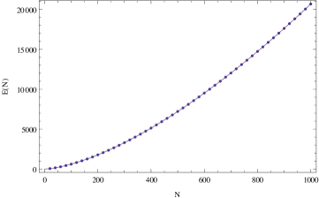
Figure 1: The function $E(N)$ (dots) versus Eq. (37) (continuous curve).

A plot of the (discretized) logarithmic derivative,

$$D(N)=\frac{\log E(N)-\log E(N-1)}{\log N-\log(N-1)}\;,$$ (38)

in Fig. 2 is clearly consistent with $\lim_{N\to\infty}D(N)=\frac{3}{2}$, in accordance with Eq. (37).

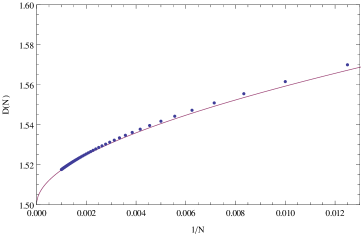
Figure 2: The dicretized logarithmic derivative $D(N)$ as a function of $1/N$ (dots) versus $\partial E(N)/\partial\log N$, with $E(N)$ given by Eq. (37) (continuous curve).

IV The three-body Coulomb case

Coming back to Eq. (12), for Coulomb interaction, one has

$$P\sum_{i<j=1}^{N}V(|z_{i}-z_{j}|)\chi = c\sum_{i<j=1}^{N}\sum_{n_{1},n_{2}=0}^{\infty}\frac{(-1)^{n_{1}}\Gamma(n_{1}+n_{2}+\frac{1}{2})}{n_{1}!\,n_{2}!\,(n_{1}+n_{2})!}\frac{(z_{i}-z_{j})^{n_{1}+n_{2}}}{2^{n_{1}+n_{2}+\frac{1}{2}}}\frac{\partial^{n_{1}+n_{2}}}{\partial z_{i}^{n_{1}}\partial z_{j}^{n_{2}}}\chi(z_{1},...,z_{N})\;$$ (39)

$$= c\sum_{i<j=1}^{N}\sum_{n=0}^{\infty}\frac{\Gamma(n+\frac{1}{2})}{(n!)^{2}2^{n}}(z_{i}-z_{j})^{n}(\partial_{j}-\partial_{i})^{n}\chi(z_{1},...,z_{N})\;.$$

This can be directly diagonalized in each sector with a given number of particles $N$ and angular momentum $L$, with the basis formed by (anti)symmetrized functions of the form (14). The general structure of the spectrum is similar to the delta interaction case: There are center-of-mass excitations, so that above each state with energy $E$ there is a “tower” with energies $E+n$, $n=1,2,\ldots$ . Only the “pure relative” eigenstates, devoid of these excitations, are of interest. We restrict ourselves to the 3-body problem. For the bosons with delta interaction, all the 3-body states turned out to have rational energies LLL (with a suitable choice of an overall factor $c$). With Coulomb interaction, though, irrational values start appearing rather low in the spectrum, for bosons and fermions like. Scaling away the overall irrationality, as before, by putting $c=\sqrt{2/\pi}$, one finds all the eigenvalues of “pure relative” states, up to the appearance of irrationalities, are, for bosons:

$L$	$E$
0	3
2	$\frac{33}{16}$
3	$\frac{51}{32}$
4	$\frac{1755}{1024}$
5	$\frac{3153}{2048}$
6	$\frac{3(27749\pm 7\sqrt{766249})}{65536}$

and for fermions:

$L$	$E$
3	$\frac{87}{64}$
5	$\frac{4881}{4096}$
6	$\frac{4119}{4096}$
7	$\frac{140283}{131072}$
8	$\frac{63255}{65536}$
9	$\frac{3(10025047\pm 3\sqrt{107141413705})}{33554432}$

V DISCUSSION

The opportunity to calculate the energy of an eigenstate of $N$ interacting two-dimensional bosons or fermions is certainly due to the fact that the LLL projection simplifies the situation. It reduces the dimension of the single-particle phase space 1D and even more importantly, the “ground state” (Bose condensate for bosons, Laughlin state for fermions) ends up being an eigenstate of the interacting Hamiltonian, which means that all one has to compute for that state is a single matrix element. Nevertheless, even this simplified setup has a physical meaning, which makes our results applicable to real systems.

The relevant case is when the LLL is separated by a gap from the rest of the spectrum. This happens when the whole system rotates with angular speed $\omega$, or if there is a strong magnetic field. But if the LLL is flat (which happens if there is a magnetic field but no harmonic potential), all the LLL $N$-body states have the same degenerate energy. Our result for the ground” state, with the minimum $L$, is valid (it still does not mix with the other states), but not meaningful physically, as that state is not separated by an energy gap from states with higher values of $L$. This changes if a harmonic potential adds $L(\omega_{t}-\omega_{\mathrm{c}})$ to the energy. One can then claim that if the interaction is weak enough compared to the gap, the exact energy of the $N$-body ground state is known.

One has to be careful, however, when taking the thermodynamic limit. As soon as $N(\omega_{t}-\omega_{\mathrm{c}})$ becomes bigger than $\omega_{\mathrm{c}}$, the energy of the lowest single-particle state in the first LL becomes smaller than that of the $N$-th single-particle state in the LLL. Actually, the LLL projection approximation breaks as soon as $N(\omega_{t}-\omega_{\mathrm{c}})\sim\omega_{\mathrm{c}}$. Therefore, for our result to be interesting, the $\omega_{\mathrm{c}}\to\infty$ limit has to be taken first, and then the thermodynamic limit $N\to\infty$.

Finally the same techniques could be applied to excited states with higher values of $L$. To do so one woud have to evaluate the matrix element $\langle p^{\prime}_{1}p^{\prime}_{2}\ldots p^{\prime}_{N}|P\sum_{i<j=1}^{N}V(|z_{i}-z_{j}|)|p_{1}p_{2}\ldots p_{N}\rangle$, where $|p_{1}p_{2}\ldots p_{N}\rangle=\prod_{l=1}^{N}z_{l}^{p_{l}}$, properly symmetrized or $|p_{1}p_{2}\ldots p_{N}\rangle=\prod_{i<j=1}^{N}(z_{i}-z_{j})\prod_{l=1}^{N}z_{l}^{p_{l}}$ properly antisymmetrized.

References

(1) S. Mashkevich, S. Matveenko, S. Ouvry,
Nucl. Phys. B 763 (2007) 431.
(2) N. R. Cooper, Adv. Phys. 57, 539 (2008); A. L. Fetter, Rev. Mod. Phys. 81, 647 (2009).
(3) The Quantum Hall Effect, eds R.E. Prange and S.M. Girvin, Springer, New York (1990).
(4) A. Prudnikov, Yu. Brychkov, O. Marichev,
Integraly i Ryady. Spetsialnye funktsii (in Russian),
Moscow, Nauka, 1983, p. 478. [Note that the source contains a misprint.]
(5) L. Brink et al., Nucl. Phys. B401 (1993) 591; S. Ouvry Phys. Lett. B510 (2001) 335.