Temperature Coefficient of Resistivity in Amorphous Semiconductors

Abstract

By invoking the microscopic response method in conjunction with a reasonable set of approximations, we obtain new explicit expressions for the electrical conductivity and temperature coefficient of resistivity (TCR) in amorphous semiconductors, especially a-Si:H and a-Ge:H. The predicted TCR for n-doped a-Si:H and a-Ge:H is in agreement with experiments. The conductivity from the transitions from a localized state to an extended state (LE) is comparable to that from the transitions between two localized states (LL). This resolves a long-standing anomaly, a “kink” in the experimental $\log_{10}\sigma$ vs. T^-1 curve.

The temperature coefficient of resistivity (TCR) in disordered systems is an important physical observable, is difficult to compute, and is of technological interest for microbolometer materials for thermal imaging applicationsmotda ; str . Boltzmann or master equations are often used to calculate transport coefficients in crystalline semiconductors and semi-metals. The low carrier concentration in these materials results in a low kinetic energy of carriers. Thus the Landau-Peierls condition: the basic criterion for a kinetic approach [$\hbar/\tau<\max\{E_{F},k_{B}T\}$] cannot be satisfiedpei , where $\tau$ is the time interval between two collisions (carrier with disorder and/or phonon), and $E_{F}$ is the Fermi energy of a material. Then, neither the elastic scattering by disorder nor the inelastic scattering by a phonon has a well-defined transition probability per unit time. The situation for amorphous semiconductors (AS) is even more difficult. Due to the strong electron-phonon (e-ph) interaction for localized states, any transition involving localized state(s) requires a reorganization of the vibrational configurationepjb ; short ; pss . Energy conservation between the initial and final electronic statespei for these intrinsic multi-phonon transitions is violated more seriously than for the single-phonon processes. Thus the kinetic method is unjustified for ASpei .

In the kinetic approachma , it is often supposed that (i) electrical conduction is fulfilled by the transition from a localized state to another localized state (LL) and the transition from an extended state to another extended state (EE)str ; motda ; (ii) the transition from a localized state to an extended state (LE) and the transition from an extended state to a localized state (EL) do not directly contribute to conduction; (iii) LE and EL transitions only maintain the non-equilibrium stationary distribution of carriers between localized states and extended states during a conduction process. Although phonon-assisted delocalizationkik ; mul and photon-excited transient currenther have been considered intuitively, rigorous expressions for LE and EL transition contributions to the conductivity are not yet available.

Because the interaction between the external electromagnetic field and an AS can be expressed with additional terms in the Hamiltonian, the transport coefficients can be expressed with transition amplitudes in the Microscopic Response Method (MRM)short ; pss . Thus the long time limit required in the kinetic approachpei is avoided. In addition, the MRM categorizes transport processes with diagrams computed to any given order of residual interactionspss . We have seen that even to zero order in the residual interactions, LE and EL transitions contribute to conductivitypss . Indeed, if one calculates the electrical conductivity of an AS from the full density matrix rather than its diagonal elements (master equation), one sees that LE and EL transitions contribute directly to electrical conduction. Since the MRM is equivalent to the density matrix method of Kuboeqv , the two methods reach the same conclusion.

Disorder scattering in EE transitions driven by field has been treated in the coherent potential approximation. The conductivity from the EE transitions depends weakly on temperaturebut , and is the same order of magnitude as that from LL transitions above room temperaturemotda ; str . In this Letter we apply MRMshort ; pss to derive the contributions to conductivity from LL, LE and EL transitions solely drive by an external field. Two examples, the conductivity and TCR of a-Si:H and a-Ge:H are described.

An accurate conductivity calculation requires (i) the eigenvalues and eigenvectors of single-electron states and (ii) the eigenfrequencies and eigenvectors for each normal modepss . To express the conductivity in terms of accessible material parameters, we approximate the vibrations of an AS by a continuous medium. Although translational invariance is destroyed in AS, the standing wave modes are still well-defined. Because most amorphous materials are isotropicstr ; motda and only acoustic modes are important for the e-ph interaction in semiconductorshan , one can use $\omega_{\mathbf{k}}=\overline{c}k$ for the vibrational spectrum, where $\omega_{\mathbf{k}}$ is the angular frequency for the mode characterized by wave vector $\mathbf{k}$. $\overline{c}$ is the average speed of sound defined by $3/\overline{c}^{3}=2/c_{t}^{3}+1/c_{l}^{3}$, where $c_{t}$ and $c_{l}$ are the speeds of transverse and longitudinal sound waves, determined by the bulk and shear modulus. The Debye cutoff wave vector $k_{D}=(6\pi^{2}n_{a})^{1/3}$ is determined by the number density $n_{a}$ of atoms in an AShan . Because the displacements of atoms satisfy a wave equation, the transformation matrix $\Delta$ between the vibrational displacements $\mathbf{u}_{\mathbf{R}}$ at point $\mathbf{R}$ and the normal coordinates $\Theta_{\mathbf{k}}$ characterized by wave vector $\mathbf{k}$ is:

$$\Delta_{\mathbf{Rk}}=(2\pi)^{-3}Ve^{i\mathbf{k}\cdot\mathbf{R}},$$ (1)

where $V$ is the volume of a sample. For a-Sistr , $\overline{c}=6.21\times 10^{3}$m/s and $k_{D}=1.44\times 10^{10}$m^-1.

For simplicity, we take localized states to be spherically symmetricnev . The difference between localized states is expressed by a single-parameter localization length $\xi_{A}$motda . We will use letter $A$ with or without a natural number subscript to denote a localized state. For a localized state $A$, denote $\mathbf{R}_{A}$ as the position vector of the center, the normalized wave function is

$$\phi_{A}(\mathbf{r}-\mathbf{R}_{A})=\pi^{-1/2}\xi_{A}^{-3/2}e^{-|\mathbf{r}-\mathbf{r}_{A}|/\xi_{A}},$$ (2)

where $\mathbf{r}$ is the coordinate of the electron and localization lengthnev . Following Mott, $\xi_{A}$ is determined by the eigenvalue $E$ of localized state $\phi_{A}$nev : $\xi_{E}=(cZe^{2}/4\pi\epsilon_{0}\varepsilon)(E_{c}-E)^{-1},$ where $Z$ is the effective nuclear charge of an atom core, $\varepsilon$ is the static dielectric constant. $E_{c}$ is the mobility edge of the conduction band, and $c$ is a dimensionless constant. We will focus on n-doped material: transport in the conduction band, p-doped material may be treated analogously. For a-Sistr , $\varepsilon=11.68$, $Z=4$ and the values of $E_{c}$ are rather dispersedvis ; jj ; ora : 0.2-2eV: we will takejj $E_{c}=0.5$eV. The most localized states are dangling bonds, they have the shortest possible $\xi_{\min}=2.35/2$Å (one half of a bond length). $E=0$ for a dangling bond, then $c=0.121$. For many ASaljishi , in the range of conduction band tail, the density of localized states (DOS) satisfies

$$N(E)=(n_{loc}/U)e^{-(E_{c}-E)/U},$$ (3)

where $U$ is the Urbach energy, $n_{loc}$ is the total number of localized states per unit volume. For a-Si, $U\thickapprox 50$meVora ; weh , the number density $n_{loc}$ of localized conduction states isting $n_{loc}=5/(10.86$Å$)^{3}$. The exponential $N(E)$ implies that most localized states in a-Si have a localization length in the range 6-12Å. Denote $n$ as the carrier concentration, the Fermi energy $E_{F}$ of a weakly doped AS is:

$$E_{F}=E_{c}+U\ln(n/2n_{loc}),$$ (4)

When $n\leq 2n_{loc}$, all occupied states are localized at T$=0$K. Ansatz (3) only characterizes the band tail states. To describe dangling bonds, one can (i) introduce a reasonable DOS, e.g. a rectangle or a Gaussian; (ii) correspondingly modify $E_{F}$ and energy zero-point for extended states; (iii) add the contribution from the dangling bonds to Eqs.(6,7) in the summation(s) over localized states. In this paper we ignore the small contribution of dangling bonds to the conductivity.

In an AS, an extended state is a packet of Bloch waves of its reference crystalvky ; scm , and is labeled by the wave vector of its principal Bloch wave, or more roughly by the momentum $\mathbf{p}$ of a plane wavebut ; motda . For an AS, for which the reference crystal does not exist, a wave packet constructed from plane waves is still a reasonable approximation for an extended state. We will use letter $B$ with or without a natural number subscript to denote an extended state. Excepting EE transitions driven by an external field, we may approximate an extended state $\chi_{B_{1}}(\mathbf{r})$ by a plane wave with certain momentum $\mathbf{p}$, and its eigenenergy is that of the plane wave:

$$\chi_{B_{1}}=V^{-1/2}e^{i\mathbf{p}\cdot\mathbf{r}/\hbar},\text{ \ \ }E_{B_{1}}=p^{2}/2m,$$ (5)

where the zero-point of energy for extended states is at the mobility edge $E_{c}$. The attraction between an electron and an atom core may be approximated by a screened Coulomb potentialhan . For a-Si:Hstr , we approximate its Thomas-Fermi wave vector by the valuehan for c-Si $q_{TF}=1.7$Å^-1.

With the foregoing approximations, the velocity matrix elements in the expressions of conductivity can be computed4tsf . One can also obtain the static displacements of the atoms in a localized state induced by the e-ph interaction and the reorganization energyepjb for transitions involving localized state(s)4tsf , which are essential input for the conductivity.

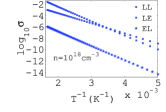
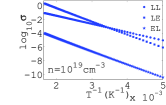
Figure 1: (color online) $\log_{10}\sigma$ vs. $1/T$ in two n-doped a-Si:H samples at $\omega=0$ with carrier concentration $10^{18}$ and $10^{19}$cm^-3. The unit of $\sigma$ is ohm^-1cm^-1.

We first calculate the conductivity from the LE transitions (line 2b of Table 4 in Ref.pss ). When $k_{B}T\geq\hbar\overline{\omega}$ (the first peak of vibrational spectrum, $\hbar\overline{\omega}=$ 232K for a-Sikam ), the two time integrals I${}_{B_{1}A\pm}$ can be approximated by an asymptotic expansion4tsf , and the vibrational degrees of freedom are integrated out. For LE transitions, we first sum over final electronic states $\sum_{B}$ for a fixed localized state $A$. It is convenient to use a spherical coordinate system with $\mathbf{R}_{A}$ as the origin and the wave vector direction $\mathbf{k/|k|}$ of the incident electromagnetic wave as polar axis (z axis)4tsf . Because AS are isotropic, the angular part of the $\mathbf{p}$ integral can be carried out. One can show that $\sigma_{xy}=\sigma_{yx}=0$ and $\sigma_{xx}=\sigma_{yy}=\sigma$. Because (i) the center $\mathbf{R}_{A}$ of $\phi_{A}$ must be a neighbor of the observation point of current density, and (ii) the factors in the conductivity do not depend on $\mathbf{R}_{A}$, $\sum_{A}\rightarrow\frac{4\pi}{3}\overline{\xi}^{3}\int_{-\infty}^{E_{c}}dEN(E)$, where $\overline{\xi}=cZe^{2}/(4\pi\epsilon_{0}\varepsilon U)$ is the most probable localization length. For a-Si, $\overline{\xi}=11.75$Å, is quite close to the experimental valueqg ; stut 10Å. The conductivity from LE transitions is4tsf :

$$\left\{\begin{array}[]{c}Re\\ Im\end{array}\right.\sigma(\omega)=\frac{cZe^{2}(n_{loc}\frac{4\pi}{3}\overline{\xi}^{3})}{4\pi\epsilon_{0}\varepsilon U}\frac{8ne^{2}}{3\pi\hbar^{3}m^{2}}\int_{0}^{\infty}d\xi f(E_{A})$$

$$\int_{0}^{\infty}dp[1-f(E_{B_{1}})]\frac{p^{4}}{(E_{B_{1}}^{0}-E_{A}^{0})}\frac{\xi\exp(-\frac{cZe^{2}}{4\pi\epsilon_{0}\varepsilon U\xi})}{(1+p^{2}\xi^{2}/\hbar^{2})^{4}}$$ (6)

$$\frac{\sqrt{\pi}\hbar}{2(k_{B}T\lambda_{BA})^{1/2}}[e^{-\frac{\lambda_{BA}}{4k_{B}T}(1+\frac{\hbar\omega_{BA}-\hbar\omega}{\lambda_{BA}})^{2}}\pm e^{-\frac{\lambda_{BA}}{4k_{B}T}(1+\frac{\hbar\omega_{BA}+\hbar\omega}{\lambda_{BA}})^{2}}],$$

where $\theta_{\alpha}^{A}=(M_{\alpha}\omega_{\alpha}/\hbar)^{1/2}\Theta_{\alpha}^{A}$epjb and $\hbar\omega_{BA}=E_{B}-E_{A}$. $\lambda_{BA}=\frac{1}{2}\sum_{\alpha}\hbar\omega_{\alpha}(\theta_{\alpha}^{A})^{2}$ is the reorganization energy for transition $\phi_{A}\rightarrow\chi_{B}$epjb . One can show that $\lambda_{BA}$ decreases with $\xi_{A}$.

Next we consider the conductivity from EL transitions driven by a field (line 6a of Table 5 in Ref.pss ). Because the field-matter coupling is Hermitian, the conductivity for EL transition driven by a field may be obtained from Eq.(6) by exchanging $\phi_{A}$ and $\chi_{B}$ and noticing that $\lambda_{AB}=\lambda_{BA}$. For the LE transition driven by transfer integral and the EL transition driven by e-ph interaction, one does not have this symmetryepjb ; pss .

To obtain the conductivity from LL transitions (line 2a of Table 4 in Ref.pss ), the velocity matrix elements $w_{\parallel}^{AA_{1}}$ and $v_{\parallel}^{A_{1}A}$ are computed with approximation (2) in a spherical coordinate system with $\mathbf{R}_{A}$ as origin and $\mathbf{R}=\mathbf{R}_{A_{1}}-\mathbf{R}_{A}$ as polar axis4tsf ; they exponentially decay with $R=|\mathbf{R}|$. $\sum_{AA_{1}}$ can be carried out by4tsf first considering a fixed $\phi_{A}$ and scanning $\phi_{A_{1}}$ at all possible $R$ with different $\xi_{A_{1}}$. The conductivity from LL transition driven by field becomes4tsf

$$\left\{\begin{array}[]{c}Re\\ Im\end{array}\right.\sigma(\omega)=\frac{4\pi}{3}\overline{\xi}^{3}[\frac{cZe^{2}n_{loc}}{4\pi\epsilon_{0}\varepsilon U}]^{2}\int_{0}^{\infty}\frac{d\xi_{1}}{\xi_{1}^{2}}\exp(-\frac{cZe^{2}}{4\pi\epsilon_{0}\varepsilon U\xi_{1}})$$

$$\int_{0}^{\infty}\frac{d\xi_{2}}{\xi_{2}^{2}}\exp(-\frac{cZe^{2}}{4\pi\epsilon_{0}\varepsilon U\xi_{2}})[1-f(E_{A_{1}})]f(E_{A})$$

$$\frac{\sqrt{\pi}\hbar}{2(\lambda_{A_{1}A}k_{B}T)^{1/2}}[e^{-\frac{\lambda_{A_{1}A}}{4k_{B}T}(1+\frac{\hbar\omega_{A_{1}A}-\hbar\omega}{\lambda_{A_{1}A}})^{2}}\pm e^{-\frac{\lambda_{A_{1}A}}{4k_{B}T}(1+\frac{\hbar\omega_{A_{1}A}+\hbar\omega}{\lambda_{A_{1}A}})^{2}}]$$

$$\int_{0}^{R_{c}}R^{2}dR\frac{4\pi}{3}ne^{2}\frac{(w_{\parallel}^{AA_{1}}-v_{\parallel}^{A_{1}A})(v_{\parallel}^{A_{1}A})^{\ast}}{2(E_{A}^{0}-E_{A_{1}}^{0})},$$ (7)

where $R_{c}$ is the radius of physical infinitesimal volume elementspss . $\lambda_{A_{1}A}=\frac{1}{2}\sum_{\alpha}\hbar\omega_{\alpha}(\theta_{\alpha}^{A_{1}}-\theta_{\alpha}^{A})^{2}$ is the reorganization energy for transition $\phi_{A}\rightarrow\phi_{A_{1}}$. To simplify notation, we used $\xi_{2}$ instead of $\xi_{A_{1}}$, used $\xi_{1}$ instead of $\xi_{A}$.

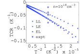
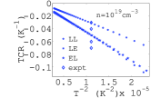
Figure 2: (color online) TCR vs. $T^{-2}$ in two n-doped a-Si:H samples at $\omega=0$ Hz with carrier concentration $10^{18}$ and $10^{19}$cm^-3, experimental values are taken from Refs.tcr ; sai ; gar .

Eqs.(6,7) express conductivity and its associated temperature dependence upon several material parameters: $n$, $n_{loc}$, $U$, $E_{c}$, $\varepsilon$, $q_{TF}$ and $\overline{c}$. Re$\sigma$ as a function of temperature T is plotted in Fig.1 for two n-doped a-Si:H samplesstr ; bey with carrier concentration $n=10^{18}$ and $10^{19}$cm^-3 [the unit of $\sigma$ is ohm^-1cm^-1]. The LE conductivity is the same order of magnitude as that from LL transitions, while the contribution from EL transitions is $10^{-4}-10^{-3}$ of that from LL transitions. Thus the calculated conductivity is the same order magnitude as the observed ones, cf. Fig.8 of Ref.sai . From Eqs.(6,7), one can easily compute the temperature coefficient of resistivity (TCR) $\varkappa=\rho^{-1}\frac{d\rho}{dT}=-\sigma^{-1}\frac{d\sigma}{dT}$. The corresponding TCR vs. T^-2 is plotted in Fig.2. If there are several processes contributing to conductivity in a material, according to MRM, the total conductivity $\sigma$ of the material is $\sigma=\sum_{j}\sigma_{j}$, where $\sigma_{j}$ is the conductivity from the j^th process (LL, LE and EL ect.)pss . The overall TCR $\varkappa$ relates to the TCR for each process by $\varkappa=\sigma^{-1}\sum_{j}\sigma_{j}\varkappa_{j}$, where $\varkappa_{j}=-\sigma_{j}^{-1}d\sigma_{j}/dT$. At 300-350K, the observed TCR is in range -0.02 to -0.08 for a n-doped a-Si:H with $n=10^{18}$cm^-3tcr ; sai ; gar . The calculated TCR from LL transitions is smaller than the experimental data, this is solid evidence that the contribution from LE transitions is important.

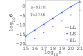
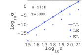
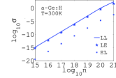
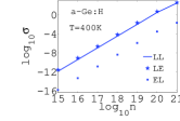
Figure 3: (color online)$\log_{10}\sigma$ vs. $\log_{10}n$ for n-doped a-Si:H and a-Ge:H. The unit of $\sigma$ is ohm^-1cm^-1, the unit of n is cm^-3.

In a-Si:H, a long-standing puzzle is (i) there is a kink in the observed $\log_{10}\sigma(T)$ vs. 1/T curve; and (ii) for very different doping concentrations, the kink temperatures collapse into a narrow rangeover . We resolve these problems. The crossing temperature $T^{\ast}$ of $\sigma_{LL}(T)$ and $\sigma_{LE}(T)$ is the key to understanding the kink. When $T<T^{\ast}$, LL transitions are the main conduction mechanism; for $T>T^{\ast}$, LE transitions dominate conductivity. If one forced a single Arrhenius fit to the overall conductivity, the formal activation energy would be different below and above T^∗. Thus one has a kink in the $\log_{10}\sigma(T)$ vs. 1/T curve. The non-exponential behavior as indicated in Eqs.(6,7) also has some role for the observed kink. For LL and LE transitions, we compute linear fits for the calculated $\log_{10}\sigma(T)$ vs. T^-1, for which the norms of the residuals are 0.03 (LL) and 0.15 (LE) for 10¹⁸cm^-3; 0.05 (LL) and 0.20 (LE) for 10¹⁹cm^-3. This is consistent with the deviation from linear relation in the measured mobility vs. 1/T curve, cf. Fig. 7.10 of str .

From Fig.1 and 1, we can see that T^∗ decreases with $n$: $T^{\ast}=$294K for 10¹⁸cm^-3, $T^{\ast}=$286K for 10¹⁹cm^-3. This is consistent with the trend found in experiments: $T^{\ast}=$400K for [PH₃]/[SiH₄]=10^-6 and $T^{\ast}=$333K for [PH₃]/[SiH₄]=10^-2, cf. Fig. 3.1 of Ref.over . Fig. 3 and 3 plot $\log_{10}\sigma$ vs. $\log_{10}n$ at T=273K and 300K. We see that at T=273K (300K), the contribution from LL transitions is larger (smaller) than that from LE transitions for carrier concentration from 10¹⁵ to 10²¹cm^-3. For very different carrier concentrations (10⁶ times different), the kink temperatures fall near 273-300K, consistent with fact (ii). In Fig. 3 and 3, we plot $\log_{10}\sigma$ vs. $\log_{10}n$ for n-doped a-Ge:H at T=300K and 400K. $T^{\ast}$s fall between 300-400K, are higher than those for a-Si:H. It agrees with the observations, compare Fig. 3.1 and 3.6 ofover .

The compositional atomic orbital and/or their relative phases for the states close to E_F in the valence band (VB) are very different to those for states close to E_F in the conduction band (CB). Because $U\varpropto\langle[(V_{a}-V_{c})/V_{c}]^{2}\rangle_{av}$ and $E_{c}\varpropto\langle(V_{a}-V_{c})/V_{c}\rangle_{av}$, where $V_{a}$ and $V_{c}$ are the potential of an AS and its reference crystalvky , $\langle\rangle_{av}$ denotes configurational and state average in ASscm . Larger $U$ and $E_{c}$ means stronger disorder, that implies smaller $\xi$ or larger $\lambda$, i.e. smaller $\sigma$ and larger $\varkappa$.

Our approach is not restricted to one component systems with weak electronic correlation. If one has a reasonable single-electron DOS in which the correlation between electrons is already taken into account, it is not difficult to calculate the e-ph coupling in multi-component system, e.g. the e-ph interaction induced by the optical modes in VO_1.83. The remaining procedure is exactly like here.

In conclusion, the microscopic response method expresses transport coefficients with transition amplitudesshort ; pss rather than transition probability per unit time, which enables the method to be used with amorphous semiconductors for which the Landau-Peierls condition is violatedpei . The conductivities from the three simplest transitions: LL, LE and EL transitions driven by field are expressed by several material parameters. The conductivity from LE transitions is as important as that from the LL transitions. The combination is responsible for the kink in the experimental $\log_{10}\sigma$ vs. $T^{-1}$ curve. The LE transition is critical in determining the TCR.

This paper provides new analytical form for $\sigma$ and $\varkappa$, suitable for amorphous semiconductors. A desirable extension would be a full ab initio evaluation of all MRM diagrams using quantities from density functional theory. This complex task is underway.

- (1) N. F. Mott and E. A. Davis, Electronic Processes in Non-crystalline Materials, Clarendon Press, Oxford, (1971).
- (2) R. A. Street, Hydrogenated Amorphous Silicon, Cambridge Univresity Press, Cambridge (1991).
- (3) R. Peierls, Surprises in Theoretical Physics, pp121-126, Princeton University Press, Princeton (1979).
- (4) M.-L. Zhang and D. A. Drabold, Eur. Phys. J. B. 77, 7-23, (2010).
- (5) M.-L. Zhang and D. A. Drabold, Phys. Rev. Lett. 105, 186602 (2010).
- (6) M.-L. Zhang and D. A. Drabold, Phys. Status Solidi B 248, 2015-2026, (2011).
- (7) A. Miller and E. Abrahams, Phys. Rev. 120, 745 (1960).
- (8) M. Kikuchi, J. Non-Cryst. Sol. 59/60, 25 (1983).
- (9) H Muller and P Thomas, J. Phys. C: Solid State Phys. 17, 5337 (1984).
- (10) H. Scher, E.W. Montroll, Phys. Rev. B 12, 2455 (1975)
- (11) M.-L. Zhang and D. A. Drabold, Phys Rev. E83, 012103 (2011).
- (12) W. H. Butler, Phys. Rev. B31, 3260, (1985).
- (13) G. D. Mahan, Many-Particle Physics, Second edition, Plenum Press, New York (1990).
- (14) N. F. Mott, Conduction in Non-Crystalline Materials, Second edition, Clarendon Press, Oxford (1993).
- (15) J. H. Davis, J. Non-Cryst. Solids 35, 67-69 (1980).
- (16) J. Dong and D. A. Drabold, Phys. Rev. Lett. 80, 1928 (1998).
- (17) F. Orapunt and S. K. O’Leary, J. Appl. Phys. 104, 073513 (2008).
- (18) S. Aljishi, J. D. Cohen, S. Jin and L. Key, Phys. Rev. Letter 64, 2811 (1990).
- (19) R. B. Wehrspohn, S. C. Deane, I. D. French, I. G. Gale, M. J. Powell and R. Brüggemann, Applied Physics Letters 74, 3374 (1999).
- (20) taken from Y.-T. Li and D. A. Drabold’s unpublished calculation on a-Si models with 64 and 216 atoms.
- (21) B. Velicky, Phys. Rev. 184, 614 (1969).
- (22) M.-L. Zhang and D.A. Drabold, Phys. Rev. B78, 195208 (2008).
- (23) M.-L. Zhang and D.A. Drabold, to be submitted to Phys. Rev. B.
- (24) W. A. Kamitakahara, C. M. Soukoulis and H. R. Shanks, U. Buchenau and G. S. Grest, Phys. Rev. B 36, 6539 (1987).
- (25) Q. Gu, E.A. Schiff, J. Chevrier and B. Equer, Phys. Rev. B52, 5695 (1995).
- (26) M. Stutzmann and J. Stuke, Solid State Communications, 47, 635-639 (1983).
- (27) W. Beyer and H. Mell, in Amorphous and Liquid Semiconductors, p.333, ed. by W. E. Spear, CICL, Edinburgh (1977).
- (28) M. B. Dutt and V. Mittal, J. Appl. Phys. 97, 083704 (2005).
- (29) D. B. Saint John, H.-B. Shin, M.-Y. Lee, S. K. Ajmera, A. J. Syllaios, E. C. Dickey, T. N. Jackson, and N. J. Podraza, J. Appl. Phys.110, 033714 (2011).
- (30) H. Overhof and P. Thomas, Electronic Transport in Hydrogenated Amorphous Semiconductor, Sec. 3.1, Springer-Verlag, Berlin (1989).
- (31) M. Garcia, R. Ambrosio, A. Torres, A. Kosarev, Journal of Non-Crystalline Solids 338–340, 744–748 (2004).