Kepler-21b: A 1.6R_Earth Planet Transiting the Bright Oscillating F Subgiant Star HD 179070

Abstract

We present Kepler observations of the bright (V=8.3), oscillating star HD 179070. The observations show transit-like events which reveal that the star is orbited every 2.8 days by a small, 1.6 $R_{\rm Earth}$ object. Seismic studies of HD 179070 using short cadence Kepler observations show that HD 179070 has a frequency-power spectrum consistent with solar-like oscillations that are acoustic p-modes. Asteroseismic analysis provides robust values for the mass and radius of HD 179070, 1.34$\pm$0.06 M_⊙ and 1.86$\pm$0.04 R_⊙ respectively, as well as yielding an age of 2.84$\pm$0.34 Gyr for this F5 subgiant. Together with ground-based follow-up observations, analysis of the Kepler light curves and image data, and blend scenario models, we conservatively show at the $>$99.7% confidence level (3$\sigma$) that the transit event is caused by a 1.64$\pm$0.04 R_Earth exoplanet in a 2.785755$\pm$0.000032 day orbit. The exoplanet is only 0.04 AU away from the star and our spectroscopic observations provide an upper limit to its mass of $\sim$10 $M_{\rm Earth}$ (2-$\sigma$). HD 179070 is the brightest exoplanet host star yet discovered by Kepler.

1 Introduction

The NASA Kepler mission, described in Borucki et al. (2010a), surveys a large area of the sky spanning the boundary of the constellations Cygnus and Lyra. The prime mission goal is to detect transits by exoplanets as their orbits allow them to pass in front of their parent star as viewed from the Earth. Exoplanets, both large and small and orbiting bright and faint stars, have already been detected by the Kepler mission (see Borucki et al. 2010b; Koch et al. 2010a; Batalha et al. 2010; Latham et al. 2010; Dunham et al. 2010; Jenkins et al. 2010a; Holman et al. 2010; Torres et al. 2010; Howell et al. 2010; Batalha et al. 2010; Lissauer et al. 2011) and many more exoplanet candidates are known (Borucki et al. 2011).

We report herein on one of the brightest targets in the Kepler field, HD 179070 (KIC 3632418, KOI 975). This V=8.3 F6IV star has been observed prior to the Kepler mission as a matter of course for essentially all of the Henry Draper catalogue stars. Catalogue information for HD179070 provides a T_eff of 6137K (spectral type F6 IV), an Hipparcos distance of 108$\pm$10 pc, [Fe/H]=-0.15, an age of 2.8 GYr, a radial velocity of -28 km/sec and E(b-y)=0.011 mag. The age, metallicity, and color excess reported in the catalogue come from the photometric study by Nordström, et al. (2004). nothing special to distinguish it from any other stars in the HD catalogue.

HD 179070 is strongly saturated in the Kepler observations. Techniques to obtain good photometry from saturated stars are employed by the Kepler project and have been used to analyze light curves of other Kepler saturated stars (e.g., Welsh et al. 2011) While a star will saturate the CCD detectors on Kepler if brighter than V$\sim$R$\sim$11.5, collecting all the pixels which contain the starlight, including the bleed trail, allow a photometric study to be performed (see Gilliland et al. 2010a). Kepler light curves of HD179070 from the early data as well as subsequent quarters of observation have shown a repeatable transit-like event in the light curve. We will examine the nature of this periodic signal using Quarter 0 to Quarter 5 Kepler observations and will show that it is caused by a small exoplanet transiting HD 179070 with a period near 2.8 days. We will refer to the host star as HD179070 and the exoplanet as Kepler-21b throughout this paper.

Our analysis for this exoplanet follows the very complete, tortuous validation path fully described in Batalha et al. (2010). The interested reader is referred to that paper for the detailed procedures which we do not completely repeat herein. Section 2 will discuss the Kepler observations including both the light curves and the pixel image data. §3 & §4 discuss ground-based speckle and spectroscopic follow-up observations we have obtained and Section 5 presents the asteroseismic results. Using a full analysis of the observations, we produce a transit model fit for the exoplanet, determine many observational properties for it, and end with a discussion of our results.

2 Kepler Observations

2.1 Kepler Photometry

The Kepler mission and its photometric performance since launch are described in Borucki et al. (2010a) while the CCD imager on-board Kepler is described in Koch et al. (2010b) and van Cleve (2008). The Kepler observations of HD 179070 used herein consist of data covering a time period of 460 days or Kepler observation Quarters 0 through 5 (JD 2454955 to 2455365). The photometric observations were reduced using the Kepler mission data pipeline (Jenkins et al. 2010b) and then passed through various consistency checks and exoplanet transit detection software as described in Van Cleve (2009) and Batalha et al. (2011). Details of the Kepler light curves and the transit model fitting procedures can be found in Howell et al. (2010), Batalha et al. (2011) and Rowe et al. (2006).

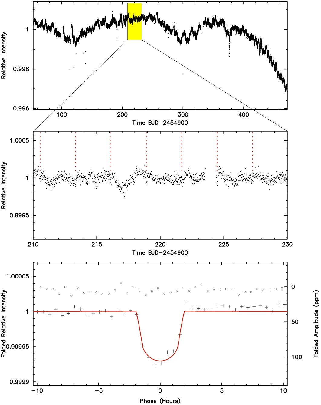
Figure 1: Kepler light curve of HD 179070 covering Quarters 0 to 5. The top raw light curve covers 164 separate transit events for the small exoplanet orbiting the star. The middle panel shows a typical normalized section from the full light curve in which transits are visible (positions marked with dotted lines). The bottom panel shows the detrended, binned, and phase folded-data (see §6) overplotted by our model fit (red line).

The top panel of Fig. 1 shows the raw Kepler light curve of HD 179070 where the larger, low frequency modulations do not likely represent real changes in the star. Thermal jumps in the focal plane temperature near day 100, 120, and 370 are apparent (see Van Cleve 2009) due to safeing events in Q2 and Q5. Normalized and phase-folded light curves are produced and the transit event in the phased light curve is modeled in an effort to understand the transiting object. The middle panel of Fig. 1 shows a blow up (as highlighted in yellow) of a section of the raw light curve and represents a typical normalized result. The dotted lines mark the individual transit events and the entire Kepler light curve shown here contains 164 individual transits. Taking random quarters of the total light curve and binning them on the transit period provide consistent results as shown in the bottom panel of Fig. 1 albeit of lower S/N. The bottom panel (Fig. 1) shows the entire phase folded light curve after detrending and binning all available data. Each bin has a width of 30 minutes and the red curve shows our transit model fit to the data. Points marked with ’o’s show where the exoplanet occultation would occur for a circular orbit (i.e., light curve phased at 0.5) or where evidence of a secondary eclipse would be seen if the event arises from a blended, false-positive eclipsing binary.

Due to the sparse (30-minute) sampling of the image data over the 3.4 hour long transit as well as the low S/N of any individual transit event, a search for transit timing variations produced no detectable periodic signal with an amplitude of 8 mins or greater and no significant deviations at all for any period.

2.2 Kepler Images and False Positive Analysis

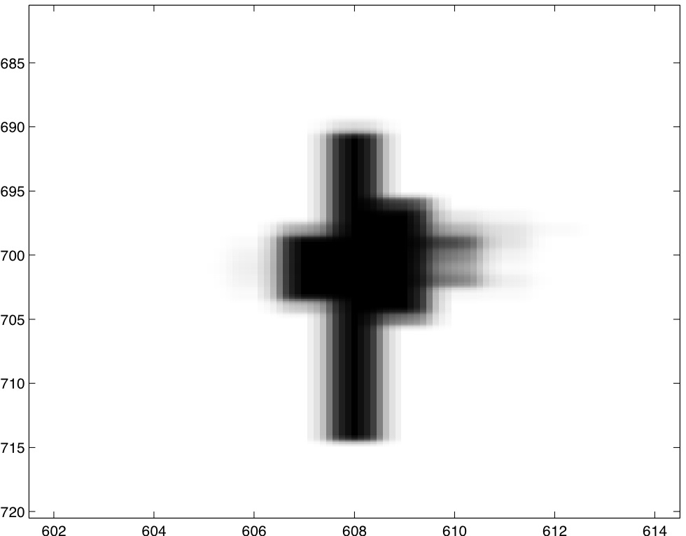
Figure 2: A typical Kepler Quarter 5 pixel image of HD 179070 showing the saturation spilled along columns and the non-saturated wings around the core.

HD 179070 is saturated in Kepler images. In a typical quarter the photometric aperture covers 128 pixels, of which 39 are typically saturated in each image. A direct pixel image of HD 179070 in quarter 5 is shown in Figure 2.

False positive identification for unsaturated Kepler targets proceeds by forming an average difference image per quarter by subtracting an average of the in-transit pixel values from average nearby out-of-transit pixel values. The resulting difference image is used to compute a high-accuracy centroid of that difference image (Torres et al. 2010). For unsaturated targets the difference image provides a star-like image at the actual location of the transiting object. The high-accuracy centroid is computed by performing a fit of the difference image to the Kepler pixel response function (PRF; see Bryson et al. 2010). When the difference images are well behaved, the centroid can have precisions on the order the PSF scale divided by the photometric signal to noise ratio of the transit signal. For Kepler-21b the SNR per quarter of about 25 would support centroiding precisions for sources near the primary of about 0.06 pixels. Having lost spatial resolution due to saturation the centroiding capability will be degraded compared to this.

The high degree of saturation of HD 179070 prevents the direct application of the above centroiding technique, but we believe that a PRF fitted centroid to the non-saturated pixels in HD 179070’s wings provide useful, albeit less accurate, results.

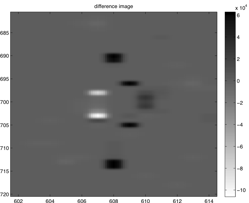
Figure 3: Kepler Quarter 5 average difference image of HD 179070 showing the pixels that change during the transit event.

Figure 3 shows the average difference image for Quarter 5, which is typical of other quarters. The pixel values which change during a transit are at the ends of the saturated columns as the amount of saturation that spills out of these ends decreases during transit. We also detect the (in phase) transit signal in the stellar wings around the core to the right of the saturated columns. Some saturated pixels become brighter on average during the transits which we ascribe to negative difference values in the pixel-level systematics linked to the non-linear behavior of saturated pixels and to large outliers caused by image motion events. Such negative difference image pixel values are commonly associated with saturated Kepler targets in which we observe shallow transits.

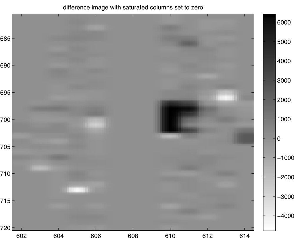
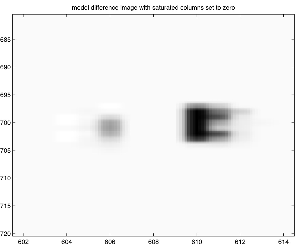
Figure 4: Left: Kepler Quarter 5 average difference image with the saturated pixels set to zero. Right: The corresponding PRF model difference image.

We can enhance our view of the stellar wings around the saturated core of HD 179070 by setting pixels in columns that have saturated pixels in the direct image to zero in the left panel of Figure 4. The right panel shows the modeled difference pixel image created by simulating the transit on HD 179070 using the PRF model of Bryson et al. (2010) and the measured transit depth, similarly setting the saturated columns to zero. We see that for the stellar wings on the right side there is a reasonable qualitative match between the modeled difference image and the observed pixel values. However, on the left side, the observed wings have slightly negative values. Since we can not know the exact center of the stellar image due to the many saturated pixels, we expect that the PRF-fitted centroid will have some x,y bias. These negative values appear for all quarters, but their locations around the core vary significantly from quarter to quarter, indicating that the PRF-fitting bias varies from quarter to quarter.

The PRF fit is performed via Levenberg-Marquardt minimization of the $\chi^{2}$ difference between the modeled and observed difference values, using non-saturated pixels in the model image whose value exceeds $10^{-4}$ of the summed model pixel values. This fit is done on both the difference and direct image, allowing us to compare the centroid of the difference image with the measured centroid of HD 179070 using the same pixels. The resulting in-transit pixel offsets are given in Table 2, with their formal uncertainties, for quarters 1, 3, 4 and 5 (no quarter 2 data are available). These uncertainties do not include the expected but unknown fit bias due to the negative values in the observed difference image. In quarter 1 we see centroid offsets exceeding a pixel, but this is almost certainly due to significant image-motion related to pixel-level systematics that were eliminated in later quarters (Jenkins et al. 2010c). In the remaining quarters the offsets are smaller, particularly in quarters 4 and 5 where the offsets are less than a pixel, and there is no consistency, as expected, in the offsets.

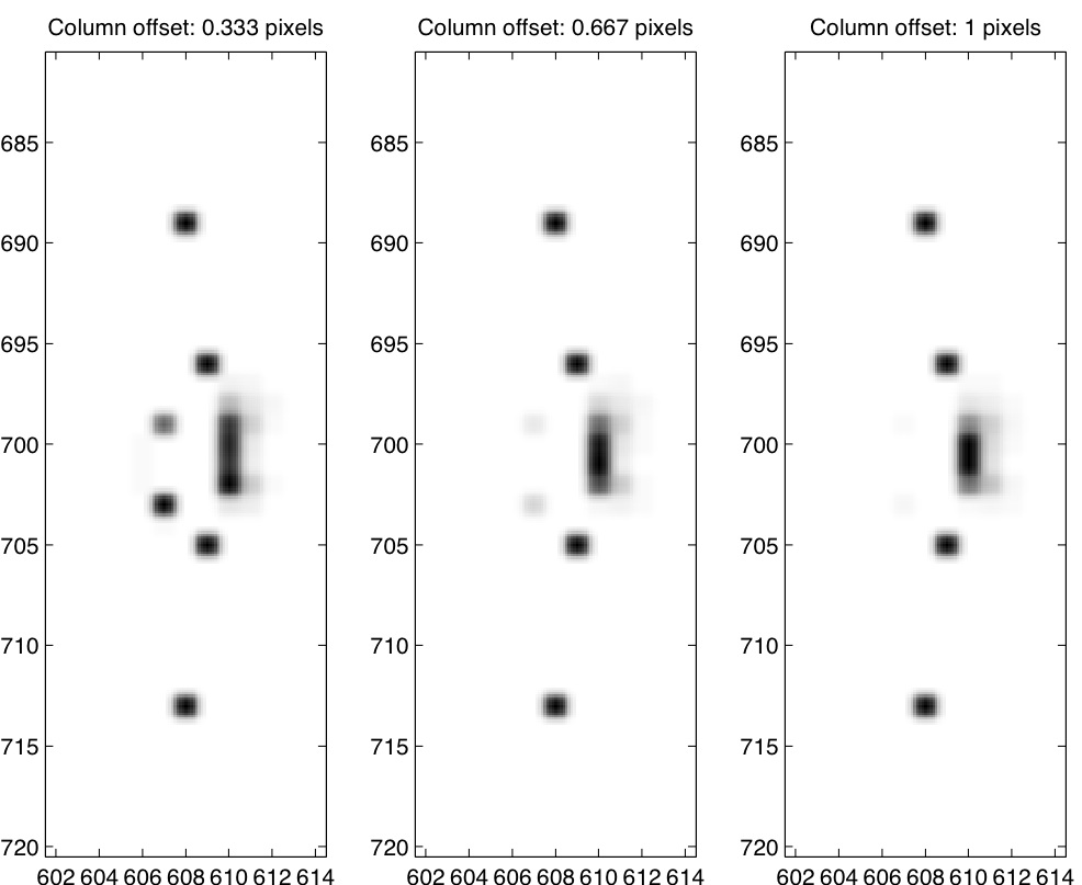
Figure 5: Quarter 5 model difference images in which the modeled faint background eclipsing binary star was offset in the column direction from the center location of HD 179070. As the column offset increases (left to right) the difference signal in the left most saturated pixels goes away. A similar result is seen for a column shift to the left.

To gain confidence in PRF fitting using pixels in the stellar wings and in using the Kepler image data for HD 179070 as a way to set limits on possible background sources which could make this a false positive, a series of modeled centroids was produced. The source of the false positive event was modeled to be caused by a very dim variable test star (e.g., a background eclipsing binary) with a Kepler magnitude of 18 in which a variation (eclipse) was added with a depth of 50%. Models were produced with the faint test star placed at various pixel positions near the expected center of HD 179070 but such that some of the test stars’ light would spill into the unsaturated wings. While the models did not exactly reproduce the observed data due to unknown systematics, the location of the saturated columns was faithfully reproduced when the transit was assumed to be on HD 179070. When the transit was placed on a background star offset by more than half a pixel in column the saturated column clearly became inconsistent with the data. When the transiting object is offset by a pixel or more in the row direction the location of the wings in the model data became similarly inconsistent with the observed data. In this way the models show that the observed difference image can clearly rule out the possibility that the transiting object is located more than a pixel (4 arcsec) from HD 179070. Row offsets displace the model stellar wings in a difference image by large fractions of a pixel relative to the observed difference images. The effect of a column offset is shown in Figure 5, where we see that a column offset of one pixel (or more) causes the transit signal in the difference image to disappear from one or more of the saturated columns again not consistent with the Kepler observations. Based on our PRF model results, we are confident that the source of the transiting object is $\leq$1 pixel of the x,y position of HD 179070.

3 High Resolution Imaging

3.1 Speckle Observations

A major part of the Kepler follow-up program (Batalha et al. 2010) used to find false positives as well as provide “third light” information to aid in Kepler image analysis is speckle imaging. We perform our speckle observations at the 3.5-m WIYN telescope located on Kitt Peak where we make use of the Differential Speckle Survey Instrument, a recently upgraded speckle camera described in Horch et al. (2010). Our speckle camera provides simultaneous observations in two filters by employing a dichroic beam splitter and two identical EMCCDs as the imagers. We generally observe simultaneously in ”V” and ”R” bandpasses where ”V” has a central wavelength of 5620Å , and ”R” has a central wavelength of 6920Å , and each filter has a FWHM=400Å. The details of how we obtain, reduce, and analyze the speckle results and specifics about how they are used eliminate false positives and aid in transit detection are described in Torres et al. (2010), Horch et al. (2010), and Howell et al. (2011).

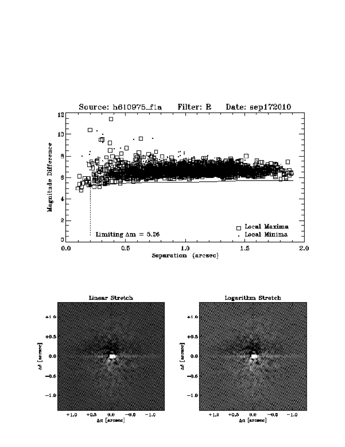
Figure 6: Speckle observation of HD 179070 showing that no line-of-sight or real companions exist from 0.05 to 2.8 arcsec of the star to a limit of 5.3 magnitudes in R (5.0 magnitudes in V) fainter than the star itself. The reconstructed images at the bottom of the plot have N up and E left. The horizontal line in the top plot shows the 5 sigma detection limit for companions against the sky background (open squares) and the vertical line at 0.2 arc seconds is added to show the inner limit for conservative multi-fringe speckle detections.

The speckle observations of HD 179070 were obtained on 17 Sept. 2010 UT and consisted of one set of 1000, 40 msec speckle images. Our R-band reconstructed image is shown in Figure 6 and along with a nearly identical V-band reconstructed image reveals no companion star near HD 179070 within the annulus from 0.05 to 1.8 arcsec to a limit of (5$\sigma$) 5.3 magnitudes fainter than the target star (that is brighter than R$\sim$13.6). At the distance of HD 179070 (d$\sim$108 pc), this annulus corresponds to distances of 5.4 to 194 AU from the star. We note that any stellar companions or massive exoplanets ($\sim$20 Earth masses or more) inside 5.4 AU would be easily detectable in the radial velocity signature (see §4). We note that while reaching to 5 magnitudes fainter than the target star eliminates bright companions and some fraction of low-mass faint associated companions, it does not completely rule out the probable larger population of faint background EBs (see §7).

3.2 MMT AO Imaging

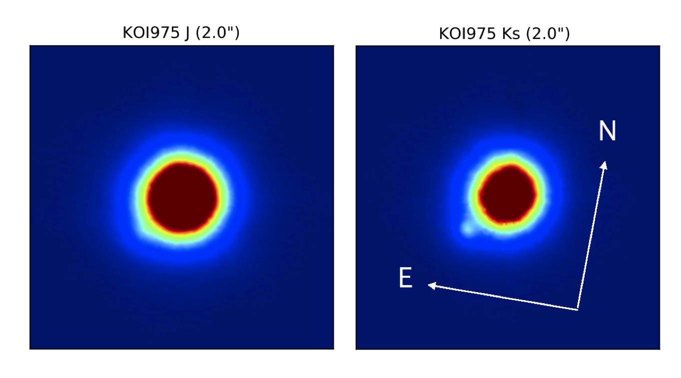
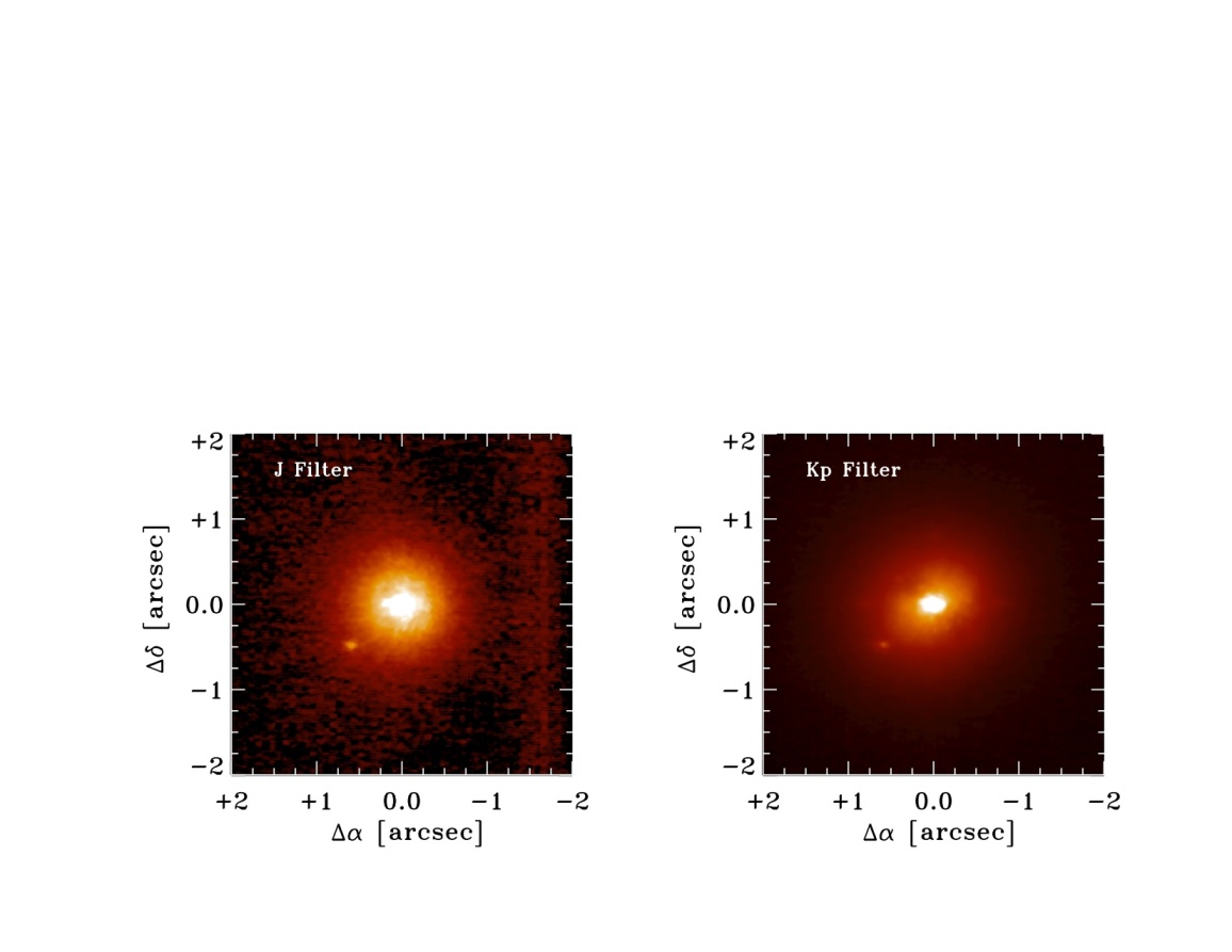
Figure 7: (top) ARIES AO images of HD 179070 in $J$ (left) and $Ks$ (right). The inner 2” are shown, along with approximate N-E axes. The companion star is clearly visible to the south-east of the main star in $Ks$, and is suggested by a slight bump at the same location in $J$. No other stars are seen within 10”. (bottom) $J$ and $K^{\prime}$ Keck-NIRC2 adaptive optics images of Kepler-21b. The images are centered on the primary target; the faint companion star can be seen approximately $0.75\arcsec$ to the SE of the target.

AO images of HD 179070 were obtained on 2010 September 23 UT using the ARIES instrument on the 6.5-m MMT. ARIES is a near-infrared diffraction-limited imager, and was operated in the F/30 mode (0.02” per pixel) in both the $J$ and $Ks$ filters. The combined Ks image was created by combining 18 images: one 1-s and 17 0.9-s exposures, with two initial pointings at each exposure time and a raster of 4 4-point dithers with a jittered 2” offset between each position. The combined J image was similarly made from 17 0.9-s exposures (one single and sixteen dithered images). The images were shifted, sky-subtracted, and combined using xmosaic in the IRAF package xdimsum. The final AO images are shown in Figure 7.

The seeing was relatively poor, with image FWHM of 0.33” in $J$ and 0.29” in $Ks$. A faint companion is detectable in the $Ks$ data, and hinted at in the $J$ data. PSF fitting, using an analytical Gaussian model, found a magnitude difference of $\Delta-Ks=3.7+/-0.1$, while a lower limit was estimated for $\Delta-J>4.0$. The separation between the two components was found to be 0.7” +/- 0.05”, with an approximate position angle of 135 degrees east of north.

The faint companion was detected right at the limit of the ARIES frame, and at a distant of just over 2 FWHM. At the object’s distance, 0.7”, the estimated $Ks$ detection limit for additional companions was 4.2 mag fainter (3.6 mag in $J$), increasing to 5.7 mag in $Ks$ (5.1 in $J$) at 1”, 7.5 mag in $Ks$ (7.2 in $J$) at 2”, and 8 mag in $Ks$ (7.8 in $J$) beyond 4”. In order to get better magnitude limits and a firm $J$-band detection, additional AO images were acquired using Keck.

3.3 Keck AO Imaging

Near-infrared adaptive optics imaging of HD 179070 was obtained on the night of 22 February 2011 and 23 February 2011 with the Keck-II telescope and the NIRC2 near-infrared camera behind the natural guide star adaptive optics system. NIRC2, a $1024\times 1024$ HgCdTe infrared array, was utilized in 9.9 mas/pixel mode yielding a field of view of $\approx 10\arcsec$. Observations were performed on first night in the K-prime filter ($K^{\prime}$; $\lambda_{0}=2.124\mu$m; $\delta\lambda=0.351\mu$m), and on the second night in the $J$ filter ($\lambda_{0}=1.248\mu$m; $\delta\lambda=0.163\mu$m). A single $K^{\prime}$ data frame was taken with an integration time of 2 seconds and 10 coadds; 10 frames were acquired for a total integration time of 200 seconds. A single $J$ data frame was taken with an integration of 0.18s and 20 coadds; 10 frames were acquired for a total integration time of 36 seconds. The weather on the night of the observations was poor with occasional heavy clouds.

The individual frames were background-subtracted and flat-fielded into a single final image for each filter. The central core of the resulting point spread functions had a width of $FWHM=0.07\arcsec$ ($\approx 7$ pixels) at J and $FWHM=0.09\arcsec$ ($\approx 9$ pixels) at $K^{\prime}$. The final coadded images are shown in Figure 7. A faint source is detected $0.75\arcsec$ from the primary target at a position angle of $PA=129^{\circ}$ east of north. The source is fainter than the primary target by $\Delta J=4.70\pm 0.05$ mag and $\Delta K^{\prime}=3.95\pm 0.05$ mag. No other sources were detected within $5\arcsec$ of the primary target.

If the faint companion is a dwarf star, the $J-Ks$ color implies that it is a very late M-dwarf ($\sim$M5-M8; see Leggett et al. 2002; Ciardi et al. 2011) and would be at a distance of approximately 15$\pm$8 pc. If the companion is a giant star, the $J-Ks$ color implies that it is an M0 giant and would have an approximate distance of 10 kpc. Appendix A discusses in detail our use of the near-IR AO observation to convert the companion’s brightness into K_p = 14.4$\pm$0.2. The maximum line of sight extinction to the faint companion (as determined from the IRAS/DIRBE dust maps; see Schlegel et al., 1998) is $A_{V}\approx 0.5$ mag, which corresponds to an $E(J-Ks)\approx 0.09$ mag; such an excess would only change the implied spectral type by a single subclass (M5 dwarf and K5 giant) and would not appreciably change the derived distances. The red dwarf can be made much earlier in spectral type (and thus located at the same distance of HD 179070) but this would require significant reddening along the exact line of sight to the star which is ruled out based on the color excess listed for HD 179070 in the literature (E(b-y)=0.011). The primary target has a Hipparcos distance of $108\pm 10$ pc; thus, the faint companion, whether it is a dwarf or giant, is not physically associated with the primary target.

Source detection completeness was estimated by randomly inserted fake sources of various magnitudes in steps of 0.5 mag and at varying distances in steps of 1.0 FWHM from the primary target. Identification of sources was performed both automatically with the IDL version of DAOPhot and by eye. Magnitude detection limits were set when a source was not detected by the automated FIND routine or was not detected by eye. Within a distance of $1-2$ FWHM, the automated finding routine often failed even though the eye could discern two sources, particularly since the observations were taken in poor weather conditions. A summary of the detection efficiency as a function of distance from the primary star is given Table 1. Beyond $\approx 0.7\arcsec$, the detection limit is $\approx 6$ magnitudes fainter than the target.

4 Spectroscopic Observations

Optical spectroscopy for HD 179070 was obtained by three ground-based telescopes as part of the Kepler mission follow-up program (Batalha et al. 2010). These observations include early reconnaissance spectra to assess stellar identification, rotation, and to make a first check on binary as well as detailed high precision radial velocity work using Keck HIRES. We compare all of our ground-based spectroscopic determined values in Table 2.

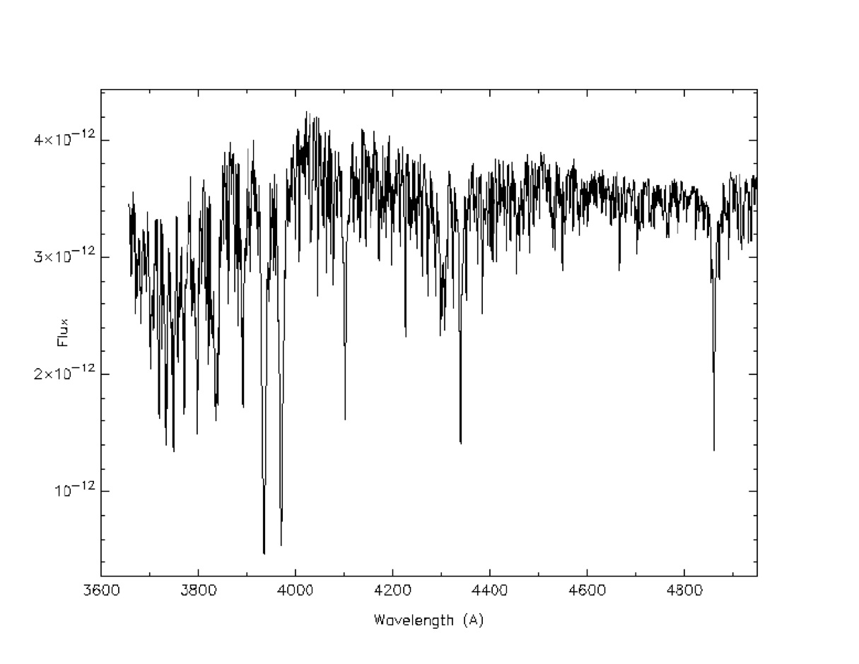
Figure 8: The Kitt Peak 4-meter spectrum of HD 179070 obtained on 16 September 2010 UT. The F6 IV star has an effective temperature of 6131K and a log g of 4.0. See Table 2.

Reconnaissance spectra of HD179070 were obtained on 13 & 16 Sept. 2010 UT at the Kitt Peak 4-m telescope using the RCSpec instrument. The 4-m RCSpec setup used a 632 l/mm grating (KPC-22b in second order) with a 1 arcsec slit to provide a mean spectral resolution of 1.6Å per resolution element across the full wavelength range of 3750-5100Å. The spectra were reduced in the normal manner with observations of calibration lamps and spectrophotometric stars (obtained before and after each sequence) and bias and flat frames collected each afternoon. Each fully reduced 4-m spectrum (see Figure 8) was cross-correlated and $\chi^{2}$ fit to both the entire MK standard stars digitally available in the “Jacoby Atlas” (Jacoby et al. 1984; covers all spectral and luminosity types) as well as to a suite of stellar models (ranging in T_eff from 3500K to 7000K, log g from 1.0 to 5.0, and solar metallicity) available through the Spanish Virtual Observatory.

Spectral type, luminosity class, and other stellar parameters were provided by the best fit match and both of the 4-m spectra gave consistent results: F4-6 IV star with T_eff = 6250$\pm$250K, log g = 4.0$\pm$0.25, and metal poor ([Fe/H] = -0.15). No relevant $vsini$ information was available from the moderate resolution (R$\sim$5000) 4-m spectra.

As is common procedure for the Kepler Mission, all exoplanet candidate stars also receive high resolution, low signal to noise (S/N), spectroscopic observations to identify easily recognizable astrophysical false positives. One or two correctly timed spectra can help rule out many types of false positives, including single- and double-lined binaries, certain types of hierarchical triples and even some background eclipsing binaries, all of which show velocity variations and/or composite spectra that are readily detectable by the modest facilities used for these reconnaissance observations. We also use these spectra to estimate the effective temperature, surface gravity, metallicity, and rotational and radial velocities of the host star. Below is a brief description of the instrument, the data reduction, and the analysis performed in this step.

We used the Tillinghast Reflector Echelle Spectrograph (TRES; Furesz 2008) on the 1.5m Tillinghast Reflector at the Fred L. Whipple Observatory on Mt. Hopkins, AZ to obtain a high resolution, low S/N spectrum of HD 179070 (S/N$\sim$7 per resolution element, 360 second exposure) on 28 Sep 2010 UT. The observation was taken with the medium fiber on TRES, which has a resolving power of $\lambda$/d$\lambda$ $\sim$ 44,000 and a wavelength coverage of 3900-8900 angstroms. The spectrum was extracted and analyzed according to the procedures outlined by Buchhave et al. (2010). Cross-correlations were performed against the grid of CfA synthetic spectra, which are based on Kurucz models calculated by John Laird and rely on a line-list compiled by Jon Morse. The template with the highest correlation coefficient yields an estimate of the stellar parameters: T_eff = 6250$\pm$125 K, log(g) = 4.0$\pm$0.25, and Vrot = 8$\pm$ 1 km/s. The errors correspond to half of the grid spacing, although they neglect possible systematics, e.g., those introduced in the event the metallicity differs from solar. We find the absolute radial velocity to be V_rad = -19.1$\pm$0.3 km/s.

Finally, HD 179070 was subjected to RV measurements with Keck (Vogt et al. 1994, Marcy et al. 2008). We note that the Ca-II K-line shows virtually no chromospheric reversal, giving an $S$ value of 0.14, placing HD 179070 among the quietest G stars. We have obtained 14 RV measurements with the Keck telescope and HIRES spectrometer (R=60,000). The exposure time for each spectrum was established by use of an exposure meter such that all would yield a consistent S/N and thus very similar RV precision. The Keck HIRES exposures were 150$\pm$30 sec in all cases. Each observation consisted of a triplet of exposures with each exposure having a signal-to-noise of 210 per pixel and an internal RV error of $\sim$2 m s^-1. We determined the RV from each exposure and took the weighted mean as the final RV for each triplet. The internal error (a typical uncertainty for each exposure) was based on the iodine line fits for each exposure.

We adopted a jitter of 5 m s^-1, typical for stars of such spectral type and rotational Vsini, adding the jitter in quadrature to the internal errors that were $\sim$2 m s^-1. Low-gravity F6 stars are well known to exhibit jitter of $\sim$5-10 m/sec (Isaacson & Fischer 2010) due presumably to photospheric velocity fields but the exact origin remains unclear. F-type main sequence stars engage in a quasi-stable $\delta$ Scuti-like phenomenon, a feature not seen in the G and K stars. Table 3 gives the times and the velocity measurements and their uncertainties. The jitter was not added to these uncertainties in quadrature, offering the reader a chance to see the uncertainties pre-jitter. The resulting 14 RVs had a standard deviation of 5.6 m s^-1, consistent with the expected total errors.

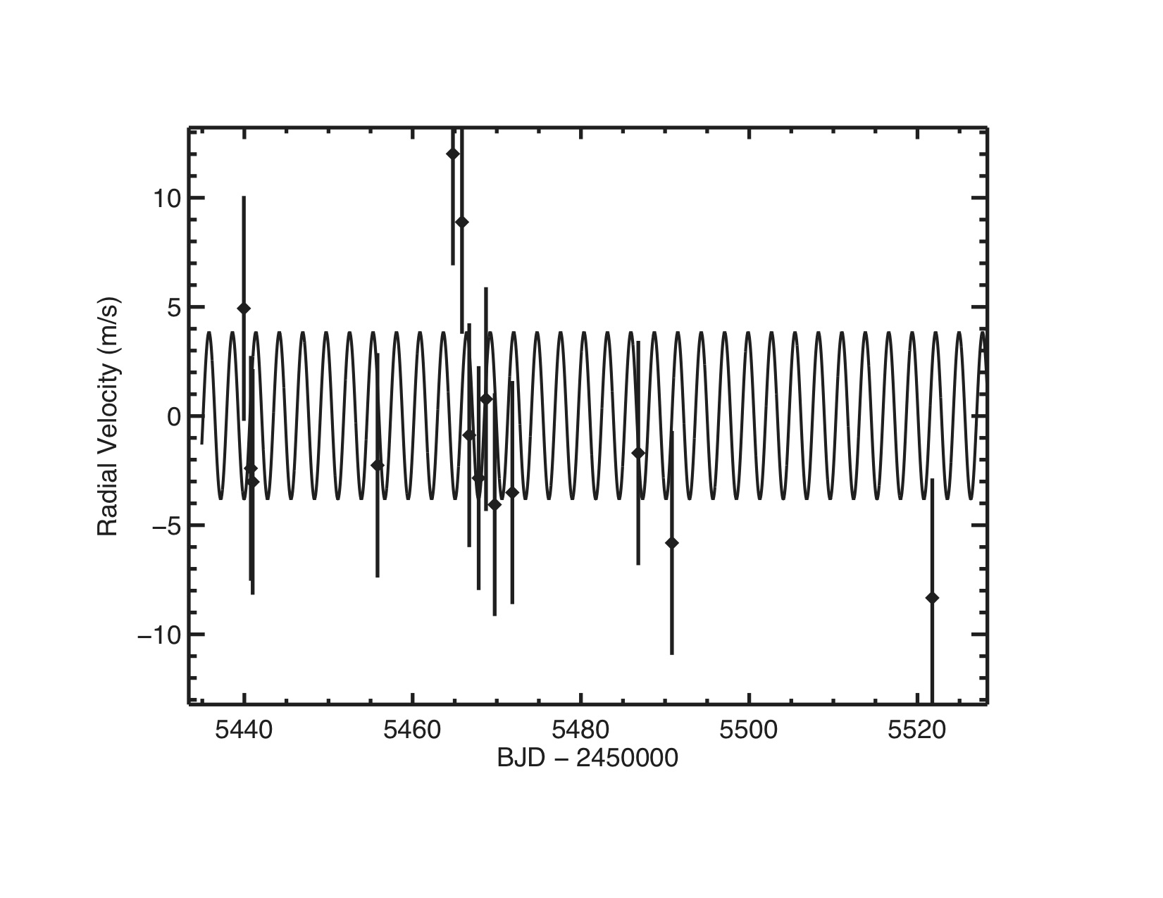
Figure 9: Radial velocity measurements for HD179070 from the Keck HIRES spectrometer are presented as a function of time. Internal errors of $\sim$2m/s are added in quadrature to 5m/s of jitter to account for uncertainty in the measurements due to spectral type. A Keplerian orbit for Kepler-21b is overplotted (see test). The radial velocity amplitude does not correlate to the expected phase of the planet nor is any additional coherent variation observed. The radial velocities therefore provide only an upper limit to the amplitude. The small RMS scatter of 5 m s^-1 imposes an upper limit on the planet mass (see text) and rules out a grazing incidence eclipsing binary.

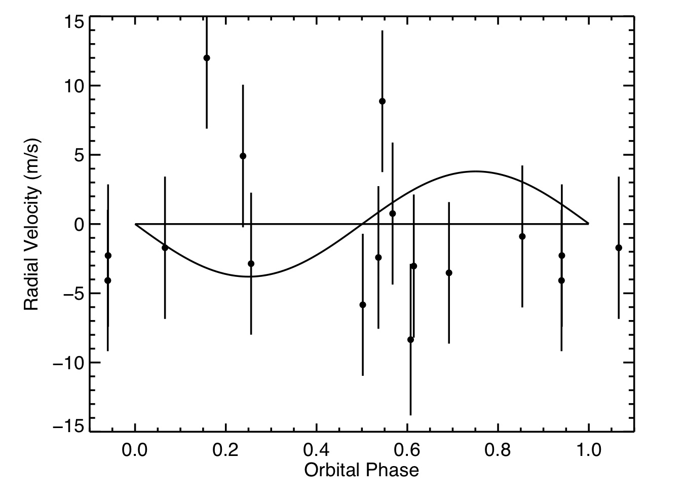
Figure 10: Keck velocities vs orbital phase for HD 179070. The velocities exhibit no evidence of coherence with orbital phase, thus offering only a 3$\sigma$ upper limit to the mass of the planet of $\sim$20 Earth-masses. The solid line shows the expected RV curve for a 10.4 Earth-mass planet orbiting HD 179070 (see §8).

In Figure 9, we show the velocities of HD 179090 measured with the HIRES spectrometer on the Keck 1 telescope during $\sim$90 days in 2010 and 2011. See Jenkins et al. (2011) and Batalha et al. (2011) for a detailed explanation of the (standard) method we used with the iodine cell to make these Doppler measurements. The velocities in Figure 9 present no clear long term variability on time scales of weeks or months. A periodogram of the velocities reveals no significant power at any period from 0.5 d to the duration of the RV observations, 85 dy, including periodicity in the velocities at the transit period of 2.7857 d. The Keck RVs are shown in Figure 10 as a function of known orbital phase (from the Kepler photometric light curve). The RV variation measured shows no modulation coherent with the orbital phase and is consistent with no change at all within the uncertainties.

We performed a standard LTE spectroscopic analysis (Valenti and Piskunov 1996; Valenti and Fischer 2005) of a high resolution template spectrum from Keck-HIRES to derive an effective temperature, $T_{\rm eff}$ = 6131 K, surface gravity, $\log{g}$ = 3.9 (cgs), metallicity, [Fe/H]=-0.05 and $Vsini$ = 7.5 km/sec. Ground-based high spectral resolution support observations of HD 179070 were also performed by the Kepler Asteroseismic Science Consortium (KASC). Two teams obtained estimates for [Fe/H]; Molenda-Zakowicz et al. (2010) listed two values (-0.15 and -0.23, and [Fe/H] = -0.15 was determined by H. Bruntt (priv. comm.) using NARVAL at Pic du Midi and the VWA analysis package. We adopt [Fe/H]=-0.15 for HD 179070 in this paper using the more reliable value recently obtained by Bruntt.

5 Asteroseismic analysis

5.1 Estimation of asteroseismic parameters

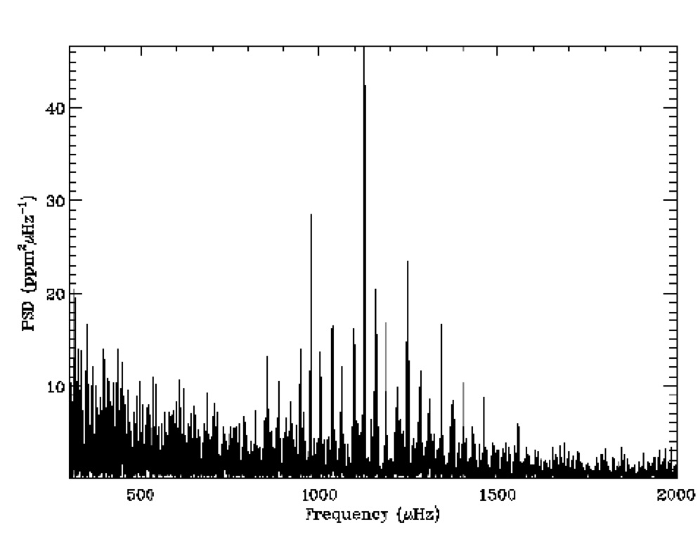
Figure 11: Frequency-power spectrum of HD 179070, showing a rich pattern of overtones of solar-like oscillations. The rising background toward lower frequencies is due to convective granulation.

HD 179070 was observed for one month by Kepler at a short cadence of 58.85 s. A time series was prepared for asteroseismic analysis in the manner described by García et al. (2011). Fig. 11 plots the frequency-power spectrum of the prepared time series, which shows a beautiful pattern of peaks due to solar-like oscillations that are acoustic (pressure, or p) modes of high radial order, $n$. The observed power in the oscillations is modulated in frequency by an envelope that has an approximately Gaussian shape. The frequency of maximum oscillation power, $\nu_{\rm max}$, has been shown to scale to good approximation as $gT_{\rm eff}^{-1/2}$ (Brown et al. 1991; Kjeldsen & Bedding 1995), where $g$ is the surface gravity and $T_{\rm eff}$ is the effective temperature of the star. The $l$ identification, from visual inspection of the mode pattern in the frequency-power spectrum, is unambiguous and the $n$ identification followed from the best-fitting to stellar evolutionary models (see below). The most obvious spacings in the spectrum are the large frequency separations, $\Delta\nu$, between consecutive overtones $n$ of the same spherical angular degree, $l$. These large separations scale to very good approximation as $\left<\rho\right>^{1/2}$, $\left<\rho\right>\propto M/R^{3}$ being the mean density of the star, with mass $M$ and surface radius $R$ (e.g. see Christensen-Dalsgaard 1993).

Here, seven teams estimated the average large separation, $\left<\Delta\nu\right>$, and $\nu_{\rm max}$, using automated analysis tools that have been developed, and extensively tested (e.g., see Campante et al. 2010a; Christensen-Dalsgaard et al. 2010; Hekker et al. 2010; Huber et al. 2009; Karoff et al. 2010; Mosser & Appourchaux 2009; Mathur et al. 2010a; Roxburgh 2009) for application to the large ensemble of solar-like oscillators observed by Kepler (Chaplin et al. 2010,2011; Verner et al. 2011). A final value of each parameter was selected by taking the individual estimate that lay closest to the average over all teams. The uncertainty on the final value was given by adding (in quadrature) the uncertainty on the chosen estimate and the standard deviation over all teams. We add that there was excellent consistency between results, and no outlier rejection was required. The final values for $\left<\Delta\nu\right>$ and $\nu_{\rm max}$ were $60.86\pm 0.55\,\rm\mu Hz$ and $1153\pm 32\,\rm\mu Hz$, respectively. We did not use the average frequency separation between the $l=0$ and $l=2$ modes (often called the small separation) in the subsequent modeling because HD 179070 turns out to be a subgiant (as indicated by, for example, the size of $\left<\Delta\nu\right>$), and in this phase of evolution the parameter provides little in the way of additional constraints given the modest precision achievable in it from one month of data (see Metcalfe et al. 2010; White et al., 2011).

Use of individual frequencies increases the information content provided by the seismic data for making inference on the stellar properties. Six teams provided estimates of individual frequencies, applying “peak bagging” techniques developed for application to CoRoT (Appourchaux et al. 2008) and Kepler data (e.g., see Metcalfe et al. 2010; Campante et al. 2010b; Mathur et al. 2010b; Fletcher et al. 2010). We implemented the procedure outlined in Campante et al. (2011) and Mathur et al. (2011) to select from the six sets of estimated frequencies one set that would be used to model the star. This so-called “minimal frequency set” contains estimates on modes for which a majority of the teams’ estimates were retained after applying Peirce’s criterion (Peirce 1852; Gould 1855) for outlier rejection. Use of one of the individual sets, as opposed to some average over all sets, meant that the modeling could rely on an easily reproducible set of input frequencies. The selected frequencies are listed in Table 4.

5.2 Estimation of stellar properties

We adopted two approaches to estimate the fundamental properties of HD 179070. In the first we used a grid-based approach, in which properties were determined by searching among a grid of stellar evolutionary models to get a best fit for the input parameters, which were $\left<\Delta\nu\right>$, $\nu_{\rm max}$, and $T_{\rm eff}=6131\pm 44\,\rm K$, from spectroscopic observations made on the Keck telescope in support of the HD 179070 analysis, and [Fe/H]$=-0.15\pm 0.06$ from Molenda-Żakowicz et al. (2011). Descriptions of the grid-based pipelines used in the analysis may be found in Stello et al. (2009), Basu et al. (2010), Quirion et al. (2010) and Gai et al. (2011).

In the second approach, the individual frequencies $\nu_{nl}$ were analyzed by the Asteroseismic Modeling Portal (AMP), a web-based tool tied to TeraGrid computing resources that uses the Aarhus stellar evolution code ASTEC (Christensen-Dalsgaard 2008a) and adiabatic pulsation code ADIPLS (Christensen-Dalsgaard 2008b) in conjunction with a parallel genetic algorithm (Metcalfe & Charbonneau 2003) to optimize the match to observational data (see Metcalfe et al. 2009, Woitaszek et al. 2009 for more details).

Each model evaluation involves the computation of a stellar evolution track from the zero-age main sequence (ZAMS) through a mass-dependent number of internal time steps, terminating prior to the beginning of the red giant stage. Exploiting the fact that $\left<\Delta\nu\right>$ is a monotonically decreasing function of age (see Metcalfe et al. 2009, and references therein), we optimize the asteroseismic age along each evolution track using a binary decision tree. The frequencies of the resulting model are then corrected for surface effects following the prescription of Kjeldsen et al. (2008). A separate value of $\chi^{2}$ is calculated for the asteroseismic and spectroscopic constraints, and these values are averaged for the final quality metric to provide more equal weight to the two types of observables. The optimal model is then subjected to a local analysis employing a modified Levenberg-Marquardt algorithm that uses singular value decomposition (SVD) to quantify the values, uncertainties and correlations of the final model parameters (see Creevey et al. 2007).

5.3 Results on stellar properties

Both approaches to estimation of the stellar properties yielded consistent results on the mass and radius of the star. The final estimates are $M=1.34\pm 0.01$(stat)$\pm 0.06$(sys)$\,\rm M_{\odot}$ and $R=1.86\pm 0.02$(stat)$\pm 0.04$(sys)$\,\rm R_{\odot}$. The statistical uncertainties come from the SVD analysis of the best-fitting solution to the individual frequencies. The spreads in the grid-pipeline results – which reflect differences in, for example, the evolutionary models and input physics – were used to estimate the systematic uncertainties.

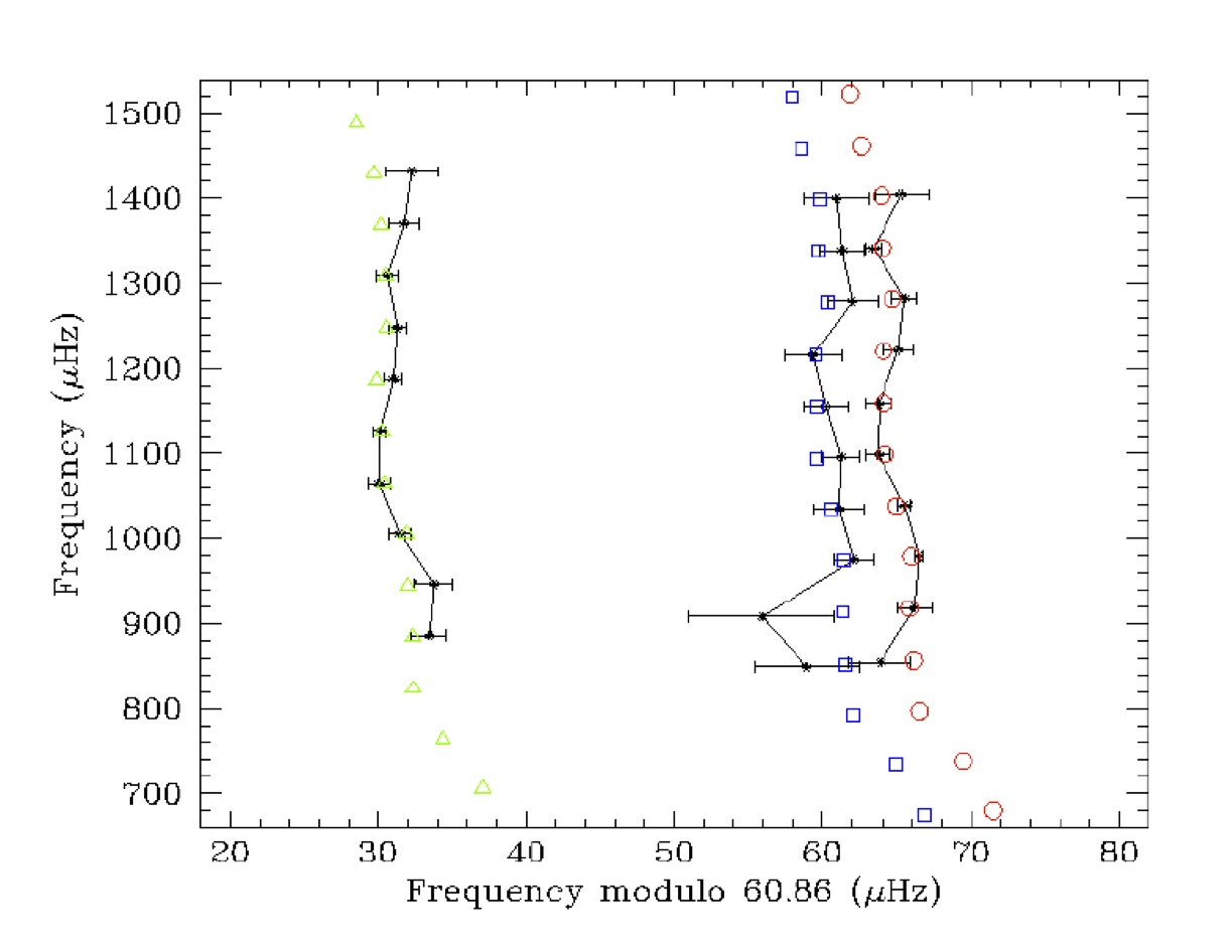
Figure 12: Echelle diagram showing the observed frequencies from Table 4, along with their $1\sigma$ uncertainties (black symbols with error bars), and the best-fitting model frequencies (color). Different symbol styles denote different spherical degrees, $l$, circles showing $l=0$, triangles $l=1$ and squares $l=2$.

The grid pipelines, which used only the average seismic parameters, showed (in some cases) two possible solutions for the age of the star (one around 3 Gyr and another around 4 Gyr or higher). Use of the individual frequencies resolved this ambiguity by giving a best-fitting solution that clearly favored the younger model, the best estimate of the age being $\tau=2.84\pm 0.10$(stat)$\pm 0.33$(sys)$\,\rm Gyr$. Fig. 12 shows good agreement between the frequencies of the best-fitting model and the observed frequencies. This échelle diagram (e.g., see Grec et al. 1983) plots the frequencies against those frequencies modulo the average large frequency separation of $60.86\,\rm\mu Hz$. Overtones of the same spherical degree $l$ are seen to align in near-vertical ridges. The observed frequencies from Table 4 are plotted in black, along with their associated $1\sigma$ uncertainties; while the best-fitting model frequencies are plotted in color.

6 Kepler Photometry Transit Fits

The raw Q1-Q5 light curve is presented in the top panel of Figure 1. The trends observed on various timescales are a combinination of astrophysical phenomenon and instrumental artifacts. These trends were removed from the lightcurve as our lightcurve model did not account for such effects. The photometric time series was prepared for modeling by independently detrending each quarterly Kepler time-series. A cubic polynomial was fitted and removed and then filtered with a 5-day running median. Any observations that occurred during transit where masked out during the calculation of the polynomial fits or medians. Our model fits for the physical and orbital parameters of the planetary system. The transit shape was described by the analytic formulae of Mandel & Agol 2002. We adopted a non-linear limb-darkening law (Claret). Coefficients were calculated by convolving Atlas-9 spectral models with the Kepler bandpass using the adopted estimate of $T_{\rm eff}$  from Table 2 and the asteroseismic value of $\log{g}$. Limb darkening coefficients are held fixed for all transit fits. We assumed a Keplerian orbit for the planet with zero eccentricity. Our model fitted for the period (P), epoch (T0), impact parameter (b), the mean stellar density ($\bar{\rho_{\star}}$), the ratio of the planet and star radii (R_p/$R_{\star}$), radial velocity amplitude (K) and the radial velocity zero point ($\gamma$). A set of best fit model parameters was constructed by fixing $\bar{\rho_{\star}}$ to the best value from asteroseimology. Minimization of Chi-squared was found using a Levenberg-Marquart method allowing P, T0, b, R_p/$R_{\star}$, K and $\gamma$

To estimate the error on each fitted parameter a hybrid-MCMC approach was used similar to Ford (2005). The asteroseismic value of $\bar{\rho_{\star}}$ and its statical error was adopted as a prior. A Gaussian Gibbs sampler was used to identify new jump values of test parameter chains. The width of the Gaussian sampler was initial determined by the error estimates from the best-fit model. After 500-chains where generated the chain success rate was examined and the Gaussian width was rescaled using Equation 8 Gregory (2011). This process was repeated after the generation of each 500 chains until the success rate for each parameter was between 22 and 28%. At which point the Gaussian width was held fixed.

To handle the large correlation between the model parameters a hybrid MCMC algorithm was adopted based on Gregory (2011). The routine works by randomly using a Gibbs sampler or a buffer of previously computed chain points to generate proposals to jump to a new location in the parameter space. The addition of the buffer allows for a calculation of vectorized jumps that allow for efficient sampling of highly correlated parameter space. After the widths Gibbs sampler stabilized, 200,000 chains where generated. The process was repeated 3 additional times to test for convergence via a Gelman Rubin test (Gelman & Rubin 1992).

The 4 chain sets where combined and used to calculate the median, standard deviation and $1\sigma$ bounds of the parameter distribution centered on the median value. Adopting the asteroseismic errors on the stellar mass and radius we computed the planetary radius ($R_{p}$), inclination angle (i) and semi-major axis (a) and also the scaled semi-major axis (a/$R_{\star}$) and transit-duration ($T_{dur}$) from the model parameter distributions and report all values in Table 5.

7 Addressing Blend Scenarios

The lack of a clear Doppler detection needed for dynamical confirmation of the nature of the transit signals in HD 179070 requires us to address the possibility that they are the result of contamination of the light of the target by an eclipsing binary falling within the photometric aperture (“blend”). The eclipsing binary may be either in the background or foreground, or at the same distance as the target in a physically associated configuration (hierarchical triple). Furthermore, the object producing the eclipses may be either a star or a planet.

We explore the wide variety of possible false positive scenarios using the BLENDER technique (Torres et al. 2004, 2011; Freesin et al. 2011), which generates synthetic light curves for a large number of blend configurations and compares them with the Kepler photometry in a $\chi^{2}$ sense. The parameters considered for these blends include the masses (or spectral types) of the two eclipsing objects (or the size of the one producing the eclipses, if a planet), the relative distance between the binary and the target, the impact parameter, and the eccentricity and orientation of the orbit of the binary, which can affect the duration of the events. Our simulations explore broad ranges in each of these parameters, with the eccentricities for planetary orbits limited to the maximum value recorded for known transiting systems with periods as short as that of HD 179070 (we adopted a conservative limit of $e<0.4$; see http://exoplanet.eu/), and eccentricities for eclipsing binaries limited to $e<0.1$ (Raghavan et al. 2010). Scenarios that give significantly worse fits than a true transit model fit (at the 3-$\sigma$ level) are considered to be rejected. While this rejection reduces the space of parameters for viable blends considerably, it does not eliminate all possible blends. Constraints from follow-up observations described previously (such as high-resolution imaging and spectroscopy) as well as multi-band photometry available for the target allow us to rule out additional areas of parameter space (see Figure 13). We then estimate the a priori likelihood of the remaining blends in the manner described in the next section. To obtain a Bayesian estimate of the probability that the transit events are due to a bona-fide planet, we must compare the a priori likelihood of such a planet and of a false positive (odds ratio). We consider the candidate to be statistically “validated” if the likelihood of a planet is several orders of magnitude greater than that of a blend. For full details on the BLENDER procedure, we refer the reader to the references cited above. Examples of other Kepler candidates validated in this way include Kepler-9 d (Torres et al. 2011), Kepler-10 c (Fressin et al. 2011), Kepler-11 g (Lissauer et al. 2011), Kepler-18 b (Cochran et al 2011), and Kepler-19 b (Ballard et al. 2011).

7.1 Background blends

We examined first the case of background eclipsing binaries composed of two stars. Our detailed simulations with BLENDER indicate that false positives of this kind are not able to match the observed shape of the transit well enough (either in depth, duration of ingress/egress, or total duration), or else they feature significant ellipsoidal variations out of transit that are not seen in the Kepler photometry. The best-fitting scenario of this kind gives a match to the observations that is worse than that of a true transiting planet model at the 6$\sigma$ level, which we consider unacceptable. We also find that blends involving evolved stars (giants or subgiants) orbited by a smaller star are easily ruled out, as well as those with a main-sequence star eclipsed by a white dwarf. In both cases the companion induces strong curvature out of eclipse due to the short orbital period (2.78 days), and for giants the large stellar radius additionally requires a grazing “V”-shaped transit to match the observed duration.

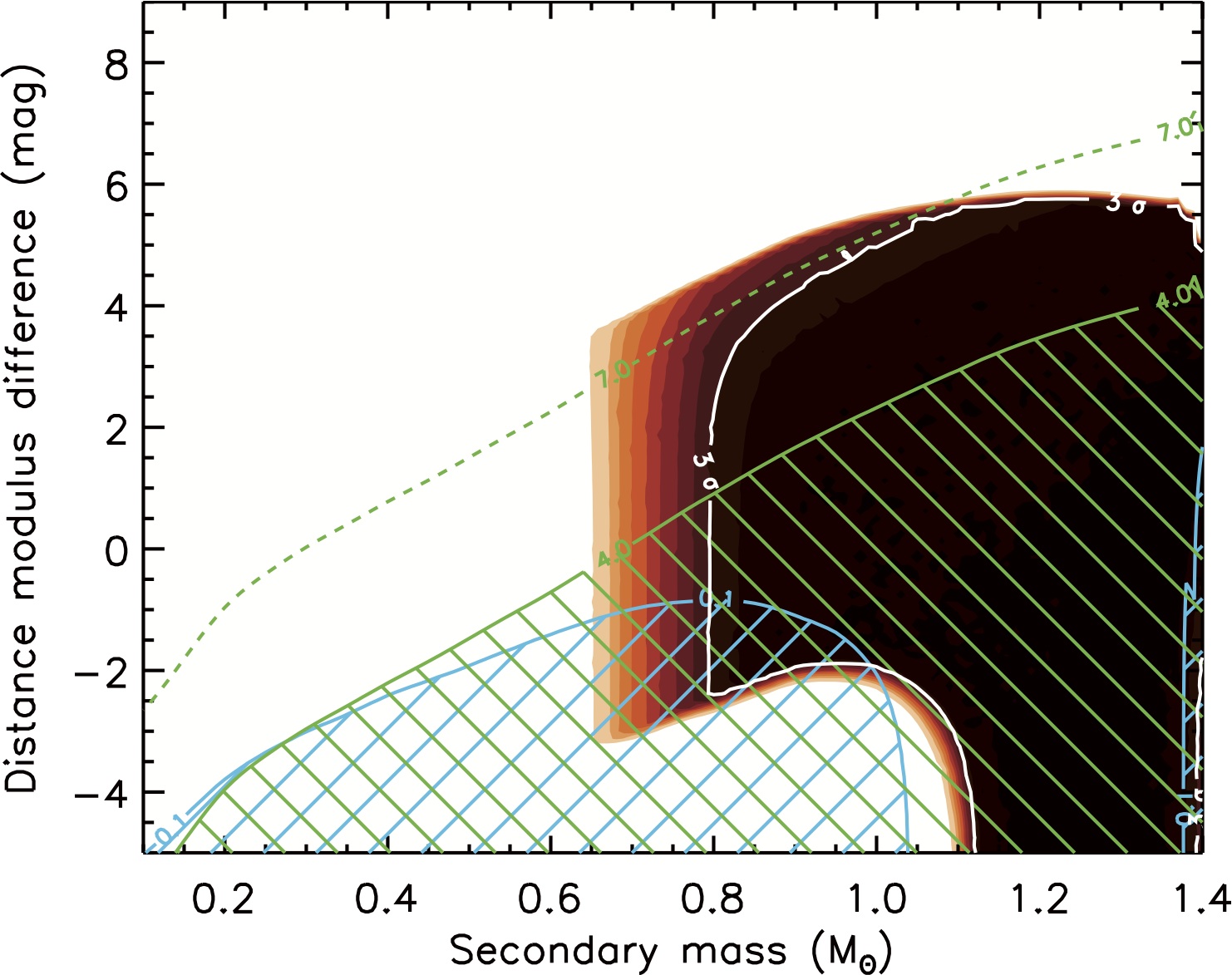
Figure 14: Map of the $\chi^{2}$ surface (goodness of fit) for blends involving background stars transited by a larger planet. The vertical axis represents the distance between the background star and the target HD 179070, expressed in terms of the difference in the distance modulus. Only blends inside the solid white contour match the Kepler light curve within acceptable limits (3$\sigma$, where sigma is the significance level of the $\chi^{2}$ difference compared to a transit model fit; see Fressin et al. 2011). Lighter-colored areas (red, orange, yellow) mark regions of parameter space giving increasingly worse fits to the data (4$\sigma$, 5$\sigma$, etc.), and correspond to blends we consider to be ruled out. The hatched blue region on the lower left corresponds to blends that can be excluded because of their overall $r\!-\!K_{s}$ colors, which are too red compared to the measured index for HD 179070, by more than 3$\sigma$ (0.10 mag). A smaller similar region is visible on the right. Blends that are bright enough to have been detected spectroscopically are indicated by the hatched green area, corresponding to contaminating stars that are up to 3 mag fainter than the target. The faintest blends that remain can be as much as 7 mag dimmer than the target (dashed green line).

When the object producing the eclipses is a planet rather than a star, ellipsoidal variations are negligible, and the shape of the eclipses (further attenuated by the light of the target) can more easily match the observed shape for a large range of properties of the stars and planets involved. An illustration of the constraints provided by BLENDER for false positives of this kind is shown in Figure 14. Following the BLENDER nomenclature we refer to the target star as the “primary”, and to the components of the eclipsing pair as the “secondary” and “tertiary” (in this case a planet). The figure shows the $\chi^{2}$ landscape (goodness of fit compared to a true transiting planet model) projected onto two of the dimensions of parameter space, corresponding to the mass of the secondary on the horizontal axis and the relative distance between the primary and the binary on the vertical axis. The latter is cast for convenience here in terms of the difference in distance modulus. The colored regions represent contours of equal goodness of fit, with the 3-$\sigma$ contour indicated in white. Blends inside this contour give acceptable fits to the Kepler photometry, and are considered viable. They involve stars that can be up to 7 magnitudes fainter than the target in the Kepler passband (as indicated by the dashed green line in the figure, corresponding to background stars with $\Delta K\!p=7$), and that are transited by a planet of the right size to produce the measured signal. Also indicated are other constraints that rule out portions of parameter space otherwise allowed by BLENDER. The blue hatched region represents blends that have overall colors for the combined light as predicted by BLENDER that are either too red (left) or too blue (right edge) compared to the measured color of the target ($r\!-\!K_{s}=1.314\pm 0.035$, adopted from the KIC; Brown et al. 2011), at the 3-$\sigma$ level. The green hatched area represents blends that are bright enough (up to 4 mag fainter than the target) to have been detected in our high-resolution spectroscopy as a second set of lines (see Sect. 4). With these observational constraints the pool of false positives of this kind is significantly reduced, but many remain. We describe in Sect. 7.3 how we assess their frequency.

7.2 Blends involving physically associated stars

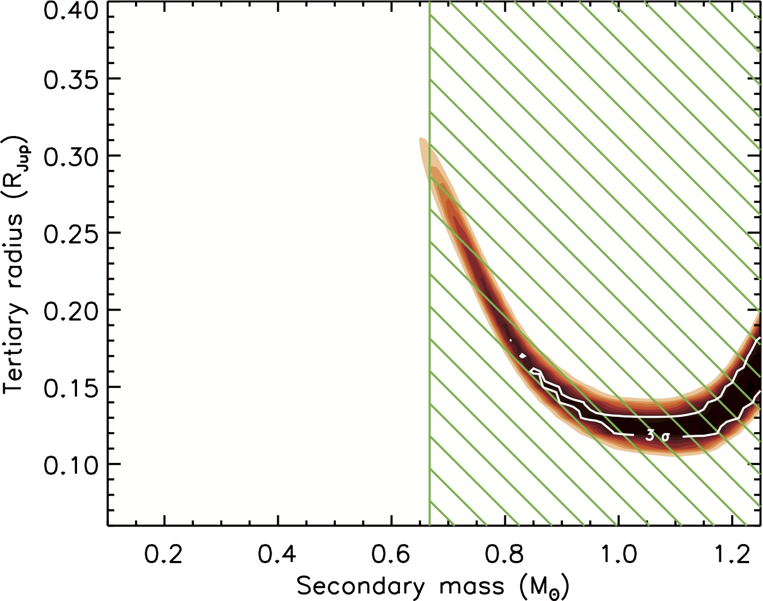
Figure 15: Similar to Figure 14 for the case of hierarchical triple systems in which the secondary star is transited by a planet, mimicking the signal in HD 179070. In this case the vertical axis represents the radius of those planets. Blends inside the white 3-$\sigma$ contour have light curves that match the shape observed for HD 179070. While the $r\!-\!K_{s}$ colors of these blends are indistinguishable from that of a single star like HD 179070 at the 3-$\sigma$ level, the stars involved are all bright enough that most would have been detected in our high-resolution spectra as a second set of lines. This is indicated by the green hatched area. Only those with a RV such that the lines are completely blended with those of the target would escape notice (see text).

Hierarchical triple configurations in which the eclipsing object (tertiary) is a star are easily ruled out by BLENDER, as these configurations invariably lead to the wrong shape for a transit. However, stars physically associated with the target that are orbited by a planet of the appropriate size can still mimic the light curve well when accounting for dilution from the brighter star HD 179070. The $\chi^{2}$ map for this type of blend is seen in Figure 15. In this case the color of the blend is not a strong discriminant, as all of these false positives are predicted to have $r\!-\!K_{s}$ indices similar to that of the target itself. The expected brightness of the companion stars, though, is such that most would have been detected spectroscopically ($\Delta K\!p\leq 4$; green hatched exclusion region), unless their RV compared to the target is small enough that their spectral lines are blended with those of the main star. Based on our spectroscopic observations we estimate conservatively that we would miss such companions if they had radial velocities within $\sim$15 km s^-1 of the RV of the target. These blends are not eliminated by any other observational constraint; we estimate their frequency below.

7.3 Validation of Kepler-21 b

With the constraints on false positives afforded by the combination of BLENDER and other follow-up observations, we may estimate the a priori likelihood of a blend following a procedure analogous to that explained by Fressin et al. (2001).

For blends involving background stars transited by a planet, this frequency will depend on the density of background objects near the target, the area around the target within which such stars would go undetected, and the rate of occurrence of planets of the appropriate size transiting those stars. We perform these calculations in half-magnitude bins, with the following ingredients: a) the Galactic structure models of Robin et al. (2003) to estimate the number density of stars per square degree, subject to the mass limits allowed by BLENDER; b) results from our adaptive optics observations to estimate the maximum angular separation ($\rho_{\rm max}$) at which companions would be missed, as a function of magnitude difference relative to the target ($K\!p=8.224$) properly converted to the $K\!p$ band, as described in the Appendix; and c) the overall frequency of suitable transiting planets that can mimic the signal. The size range for these planets, as determined in our BLENDER simulations, is 0.38–2.0 $R_{\rm Jup}$. To estimate the frequency of such planets we make use of the list of 1235 planet candidates released by the Kepler Mission (Borucki et al. (2011), based on the first four months of observation by the spacecraft. While these objects have not all yet been confirmed because follow-up is still in progress, the false positive rate is expected to be relatively low (typically less than 10%; see Morton & Johnson, 2011) and will not affect our results significantly. We therefore assume that all of them represent true planets, and that the census of Borucki et al. (2011) is complete for objects of this size (see below). The estimated frequency of these planets in the allowed radius range is $f_{\rm planet}\approx 0.19$%.

The results of our calculation for the frequency of blends involving background stars is presented in Table 6. Columns 1 and 2 give the magnitude range for background stars and the magnitude difference compared to the target; column 3 lists the range of allowed masses for the stars, based on our BLENDER simulations (see Figure 14); columns 4 and 5 list the mean star densities and $\rho_{\rm max}$, respectively, and column 6 gives the number of background stars we cannot detect, and is the result of multiplying column 4 by the area implied by $\rho_{\rm max}$. Finally, the product of column 6 and the transiting planet frequency of 0.19% leads to the blend frequencies in column 7. The sum of these frequencies is given at the bottom under “Totals”, and is $8.0\times 10^{-7}$.

For blends involving physically associated stars with RVs within 15 km s^-1 of the target, which would go unnoticed in our spectroscopic observations, we estimate the frequency through a Monte Carlo experiment. We simulate companion stars in randomly chosen orbits around the target, and randomly assign them transiting planets in the appropriate radius range as a function of the secondary mass (see Figure 15), according to their estimated frequencies from Borucki et al. (2011). We then determine what fraction of these stars would be missed because of projected angular separations below the $0\farcs 05$ detection threshold from our speckle observations, velocity differences relative to the target under 15 km s^-1, or because they would induce a drift in the RV of the target that is undetectable in our Keck observations (i.e., smaller than $\pm 10$ m s^-1 over a period of 82 days; see Sect. 4). Binary orbital periods, eccentricities, and mass ratios were drawn randomly from the distributions presented by Raghavan et al. (2010), and the mass ratios used in combination with our estimate of the mass of HD 179070 to infer the mass of the physical companions. We adopt an overall binary frequency of 34% from the same source.

Based on these simulations we obtain a frequency for this type of false positive of $1.17\times 10^{-6}$. However, as seen in Figure 15, planets involved in blends with physically associated stars can be considerably smaller ($\sim$0.12–0.18 $R_{\rm Jup}$) than those involved in background blends (0.38–2.0 $R_{\rm Jup}$), so we must consider the potential incompleteness of the census of Borucki et al. (2011) at the smaller planet sizes. To estimate this we performed Monte Carlo simulations in which we calculated the signal-to-noise ratio for each of the Kepler targets that would be produced by a central transit of a planet with the period of HD 179070 and with a given radius in the allowed range. Adopting the Kepler detection threshold of 7 for the signal-to-noise ratio Jenkins et al. (2010), we determined the fraction of stars for which such a planet could have been detected during the four months in which that sample was observed. We have assumed that the signal-to-noise ratio increases with the square root of the transit duration and with the square root of the number of transits, and that the data were taken in a continuous fashion (except for gaps between quarters). In this way we obtained a completeness fraction of about 65%, although this may be slightly optimistic given that some transits could have been missed due to additional interruptions in the data flow for attitude corrections and safe mode events. This brings the frequency of hierarchical triple blends to $1.8\times 10^{-6}$.

The total blend frequency is then the sum of the two contributions (background stars and physically associated stars with transiting planets), which is $8\times 10^{-7}+1.8\times 10^{-6}=2.6\times 10^{-6}$.

Finally, following the Bayesian approach outlined earlier, we require also an estimate of the likelihood of a true planet around HD 179070 (“planet prior”) to assess whether it is sufficiently larger than the likelihood of a blend, in order to validate the candidate. To estimate the planet prior we may appeal once again to the catalog of 1235 candidates from Borucki et al. (2011), which contains 99 systems with planetary radii within 3$\sigma$ of the measured value for HD 179070 ($R_{p}=1.64\pm 0.04\,R_{\earth}$). The 3-$\sigma$ limit used here is for consistency with a similar criterion adopted above in BLENDER. Given the total number of 156,453 Kepler targets from which the 1235 candidates were drawn, we obtain a planet frequency of $99/156,\!453=6.3\times 10^{-4}$. Applying the same incompleteness factor described above, which holds also for the radius of this candidate, we arrive at a corrected planet prior of $9.7\times 10^{-4}$. This conservative figure is $\sim$370 times larger than the blend frequency, which we consider sufficient to validate the planet around HD 179070 to a high degree of confidence. We note that this odds ratio is a lower limit, as we have been conservative in several of our assumptions. In particular, for computing the frequency of planets transiting background stars (Table 6) we have included objects with sizes anywhere between the minimum and maximum planet radius allowed by BLENDER for stars of all spectral types (0.38–2.0 $R_{\rm Jup}$), whereas the planet size range for secondaries of a given mass is considerably smaller. This would reduce the frequency of this type of false positive, strengthening our conclusion.

8 Limits to the Density and Mass for Kepler-21b

To determine a statistically firm upper limit to the planet mass, we carried out an MCMC analysis of the Keck radial velocities with a Keplerian model for the planet’s orbit. The resulting 2-sigma upper limit to the mass yielded the Keplerian model shown in Figures 9 & 10 and gave the following upper limits: RV amplitude of $K<$3.9 m s^-1; a planet mass of $M=10.4$ $M_{\rm Earth}$ (2$\sigma$), and a corresponding density of $\rho<12.9$ g cm^-3. This upper limit to the density of 12.9$gcm^{-3}$ is so high that the planet could be (compressed) solid or composed of admixtures of rocky, water, and gas in various amounts, unconstrained by this large upper limit to density. The 1-sigma upper limit to density is 7.4$gcm^{-3}$, still consistent with all types of interior compositions and would yield a planet mass of $\sim$5.9 M_Earth.

If Kepler-21b contains a large rocky core, the high pressure inside such a massive planet would cause the silicate mantle minerals to compress to dense phases of post-perovskite; the iron core is also at higher density than inside Earth (Valencia et al. 2007). However, Kepler-21b could also have a small rocky core, be mostly gas and not be nearly as massive. The maximum core fraction expected for rocky planets of this radius corresponds to a planet with mass of 10.0 M_Earth and a mean density of 12.5 g/cc (see mantle stripping simulations by Marcus et al. 2010) with a corresponding RV semi-amplitude of 2.3 m/sec, still below our detection limit. If Kepler-21b is a water planet with low silicate-to-iron ratio and 50% water by mass, its mass would be merely 2.2 M_Earth, similar to that of Kepler-11f, but at mean density of 2.7 g/cc. The measured radial velocities provide neither a confirmation nor a robust limit ($\sim$10 Earth-masses) on the mass of Kepler-21b but suggests an upper limit near that of the maximum rocky core fraction theoretically allowed. The radial velocities certainly rule out higher mass companions (additional planets or stellar companions) with orbital periods in the period range of up to approximately 200 days as any RV trend caused by such a companion would be apparent in Figs. 9 & 10.

9 Conclusion

Kepler photometry of the bright star HD 179070 reveals a small periodic transit-like signal consistent with a 1.6 R_Earth exoplanet. The transit signal repeats every 2.8 days and the complete phased light curve shows all of the events to be consistent in phase, amplitude, and duration. Analysis of the Kepler image data and difference images are well matched by model fits. Detailed point response function (PRF) models conclude that the source of the transit event is centered on or near to the center of HD 179070 itself. Furthermore, these models show that many faint background eclipsing binary scenarios, capable of blending light with that from HD 179070 to produce the transit-like event, can be eliminated.

High resolution ground-based optical speckle imaging reveals no nearby companion star to within 5 magnitudes of HD179070 itself. Near-IR AO observation, however, reveal a faint companion star 0.75” away and $\sim$4 magnitudes fainter in $K$. Using a color transformation, this star is expected to be R$\sim$14.2, just below the detection limit of the speckle results. Spectroscopic observations also confirm that no bright star is present near HD 179070 (within 0.5”). Asteroseismology was performed for HD 179070 using the Kepler light curves. Adopting the spectroscopically determined values for T_eff, log g, and [Fe/H], the mass, radius, and age of HD 179070 were well determined.

Putting all of the above observations and models together, we conclude that the cause of the periodic transit event is indeed a small 1.6 R_Earth exoplanet orbiting the subgiant star HD 179070. Transit models were fit to the highly precise Kepler light curve data revealing that the exoplanet orbits every 2.78 days at an inclination of 82.5 degrees. The exoplanet has an equilibrium temperature near 1900K and is located 0.04 AU from its host star. Kepler-21b has been validated by detailed modeling of blend scenarios as a true exoplanet at greater than 99.7% confidence. We can only determine an upper mass limit for the exoplanet, $\sim$10 M_Earth, resulting in a upper limit to the mean density of $\sim$13 g cm^-3.

Kepler continues to monitor HD 179070 and will eventually build up higher S/N phased transit light curves. These long term observations may allow other planets within this same system may be directly detected or detected via transit timing variations. Given the brightness of HD 179070, it is likely that continued radial velocity monitoring will take place with Keck or other current or planned radial velocity instruments. Given a consistent level of instrumental precision, the observed stellar jitter will slowly be averaged out and velocity signals from this or other planets orbiting the host star may be detected. Finally, using a technique such as described in Schuler et al. (2011) high-resolution, high signal-to-noise echelle spectroscopy will provide detailed metal abundance values of the host star’s atmosphere which may hold clues as to the formation, or not, of planetary bodies.

10 Appexdix A: Transformation of Infrared Colors

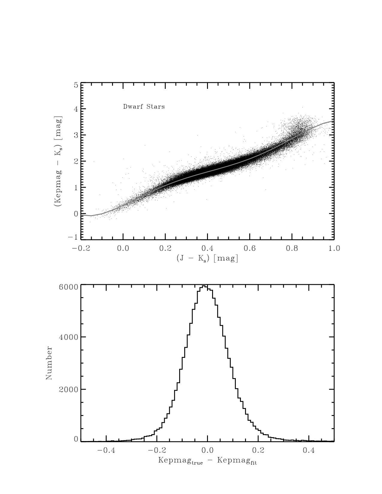
Figure 16: Top: $Kepmag-Ks$ vs $J-Ks$ for Q1 dwarf stars. The grey line represents the 5th order polynomial fit. Bottom: histogram of the residuals from the polynomial fit.

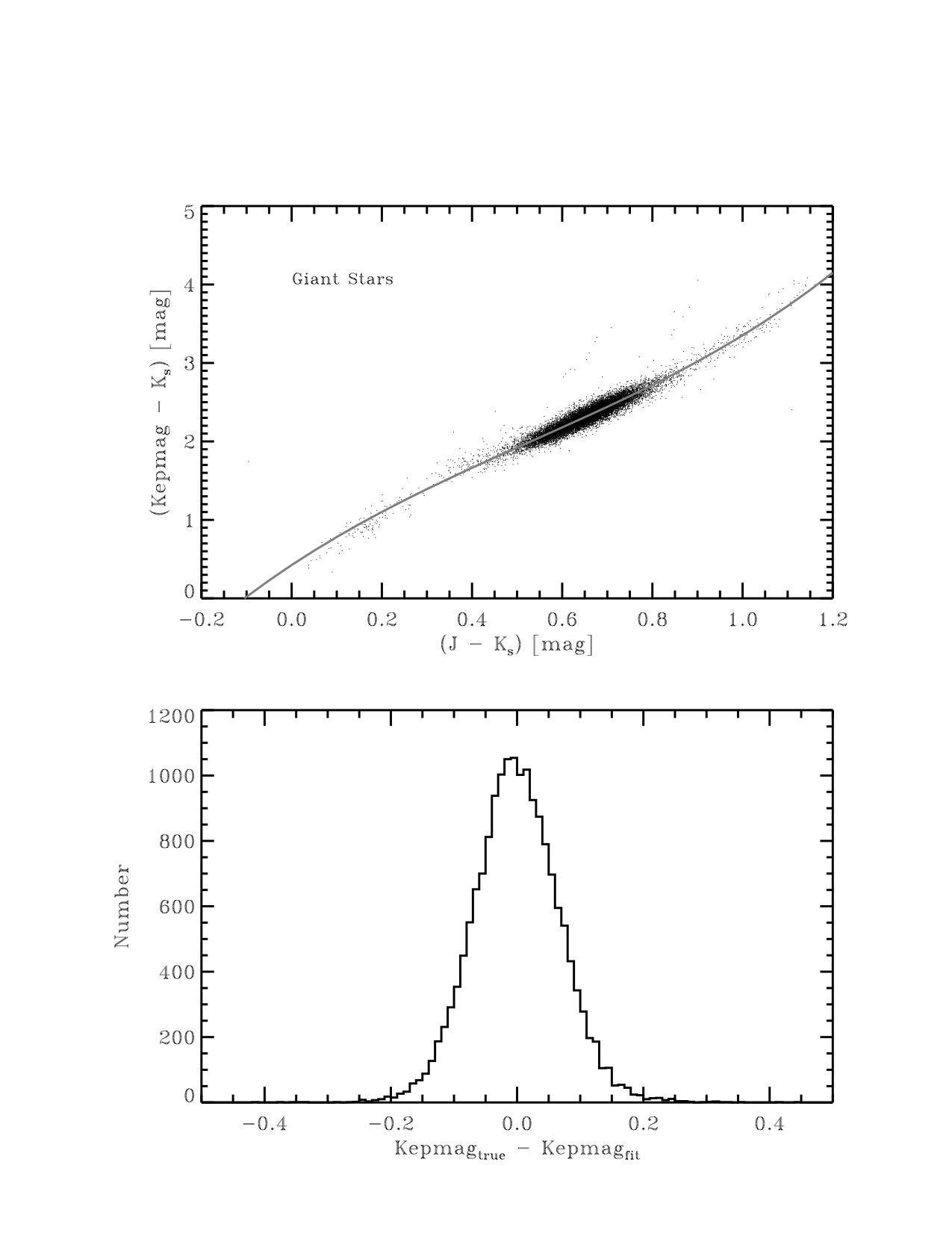
Figure 17: Top: $Kepmag-Ks$ vs $J-Ks$ for Q1 giant stars. The grey line represents the 3rd order polynomial fit. Bottom: histogram of the residuals from the polynomial fit.

To understand the contribution of the faint infrared companion to the light curve in the Kepler bandpass, we need to convert the measured infrared color ($J-K^{\prime}$) to a Kepler magnitude ($Kp$). To do this, we have derived a color-color relationship ($Kp-Ks$ vs. $J-Ks$) utilizing the Kepler targets from Q1 public release and the photometry from the Kepler Input Catalog (KIC; Brown et al. 2011). Separating the KIC into dwarfs and giants as described by Ciardi et al. (2011), we have fitted the color-color relationship with a 5th-order polynomial for the dwarfs and a 3rd-order polynomial for the giants (see Figures 16 and 17).

The dwarf and giant color-color relationships were determined separately from the Kepler magnitude and 2MASS magnitudes of 126092 dwarfs within the color range of $-0.2\leq J-Ks\leq 1.0$ mag and 17129 giants within the color range of the $-0.2\leq J-Ks\leq 1.2$ mag. The resulting polynomial coefficients from the least squares fits for the dwarfs and giants, respectively, are

$${\rm Dwarfs:\ }Kp-Ks=0.314377+3.85667x+3.176111x^{2}-25.3126x^{3}+40.7221x^{4}-19.2112x^{5}$$

$${\rm Giants:\ }Kp-Ks=0.42443603+3.7937617x-2.3267277x^{2}+1.4602553x^{3}$$

$${\rm where\ }x=J-Ks.$$

The fits and the residuals are shown in Figures 16 and 17; the residuals for both the dwarfs and giants are well-characterized by gaussian distributions with means and widths of $\langle Kp_{J-Ks}-Kp_{true}\rangle=-0.005\pm 0.083$ mag and $\langle Kp_{J-Ks}-Kp_{true}\rangle=-0.002\pm 0.065$ mag for the dwarfs and giants, respectively. The uncertainties in the derived Kepler magnitudes ($Kp$) are dominated by the physical widths of the color-color relationships.

The real apparent photometry of the infrared companion was determined from the 2MASS photometry of the primary target ($J=7.229\pm 0.032$ mag, $Ks=6.945\pm 0.018$ mag) which is a blend of the two sources. The above color-color relationships were determined using the $Ks$ filter, but the observations were taken in the $K^{\prime}$ filter which has a slightly shorter central wavelength (2.148 $\mu$m vs. 2.124 $\mu$m). Typically, the $Ks$ and $K^{\prime}$ filters yield magnitudes which are within $0.02-0.03$ magnitudes of each other and have zero-point flux densities within 2% (AB magnitudes = 1.86 and 1.84 for $Ks$ and $K^{\prime}$, respectively; Tokunaga & Vacca 2005). Given the quality of the weather and resulting photometry, the width of the color-color relationships, and lack of an $H$-band observation to aid in the transformation of the $K^{\prime}$ observations, we have equated $K^{\prime}$ to $Ks$ in these calculations and propagated an additional uncertainty of 0.03 mag in the derivation of the $J-Ks$ color and the Kepler magnitude ($Kp$).

Deblending the infrared photometry results in the following infrared magnitudes for the primary target and faint companion of $J=7.24\pm 0.07$ and $11.94\pm 0.07$ mag,respectively, and $Ks=6.97\pm 0.07$ and $Ks=10.92\pm 0.07$ mag, where we have propagated the uncertainties of the faint companion on to the photometry of both stars. The infrared colors of the faint companion is $J-Ks=1.0\pm 0.1$ mag, which corresponds to a $Kp-Ks$ color of $Kp-Ks=3.54\pm 0.14$ mag if the faint star is a dwarf and a color of $Kp-Ks=3.35\pm 0.14$ mag if the faint star is a giant.

Applying the deblended $Ks$ magnitude of the companion ($Ks=10.92\pm 0.07$ mag), we derive a magnitude for the faint star in the Kepler bandpass for the dwarf- and giant-star relationships of $Kp=14.5\pm 0.2$ mag and $Kp=14.3\pm 0.2$ mag, respectively. The companion is fainter than the primary target, in the Kepler bandpass, by $\Delta Kp=6.3$ mag if the star is dwarf and $\Delta Kp=6.1$ mag if the star is a giant. Note the primary star dominates the photometry in the Kepler aperture; after deblending the Kepler magnitude of the star changes from $Kp=8.224$ mag to $Kp=8.227$ mag if the companion is a dwarf or to $Kp=8.228$ mag if the companion is a giant.

The above relationships only work if both $J$ and $Ks$ magnitudes are known, but often only one of the filters is available. Being able to convert a single $J$ and $Ks$ magnitude into an expected $Kp$ is extremely useful – particularly, for determining sensitivity limits for the AO imaging. Towards this end we have utilized the Kepler Input Catalog to determine the expected $Kp-J$ and $Kp-Ks$ colors for a given $J$ or $Ks$ magnitude.

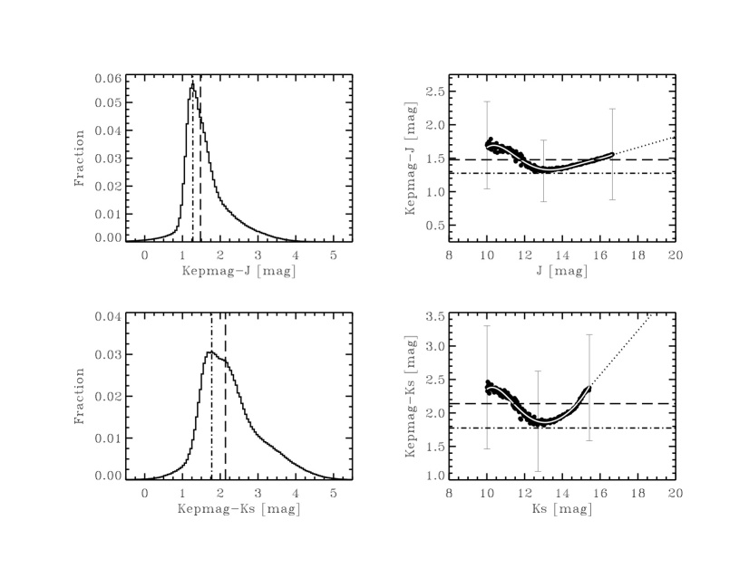
Figure 18: Top: (left) Histogram of the $Kp-J$ color for all sources in the KIC. The dashed line marks the median value and the dashed-dot line marks the peak of the histogram. (right) Median $Kp-J$ color for all sources in the KIC as a function of $J$ mag (binsize = 0.02 mag in $J$). The horizontal dashed and dashed-dot lines mark the same values as in the histogram. Three representative dispersions per bin are shown as error bars. The white solid line represents a 5th-order polynomial fit to the data, and the dotted line represents a linear fit to sources fainter than $J=15$ mag extrapolated to magnitudes beyond the limits of the KIC. Bottom: (left) Histogram of the $Kp-Ks$ color for all sources in the KIC. (right) Median $Kp-Ks$ color for all sources in the KIC as a function of $Ks$ mag (binsize = 0.02 mag in $Ks$). The various lines demark the same values as in the top plots but for $Kp-Ks$ values.

Histograms of the $Kp-J$ and $Kp-Ks$ colors are shown in Figure 18 where the median and mode of the color are marked; the spread in color, as described by the dispersion of the colors, is fairly large. The medians, modes (both of which are delineated in the histograms), and dispersions of the colors are $Kp-J=1.477$, $1.275$, and $0.626$ mag and $Kp-Ks=2.139$, $1.775$, and $0.803$ mag.

It is not unexpected that the measured median colors would be dependent upon the real apparent infrared magnitude; as the photometry becomes more sensitive to fainter and fainter sources, more intrinsically fainter (and redder) sources should contribute more significantly to the color distribution. To explore this effect, we have computed the median color ($Kp-J$ and $Kp-Ks$) as a function of the real apparent infrared magnitude (see Fig 18). The dispersion per bin is fairly large ($0.4-0.9$ mag), but the colors show smooth systematic trends as a function of magnitude with a range of $0.5-0.6$ mag.

We have characterized these curves with 5th-order polynomials and have done a linear extrapolation for magnitudes fainter than the data range:

$$Kp-J=-398.04666+149.08127J-21.952130J^{2}+1.5968619J^{3}-0.057478947J^{4}+0.00082033223J^{5}$$

for $(10<J<16.7\ {\rm mag})$

$$Kp-J=0.1918+0.08156J$$

for $(J>16.7\ {\rm mag})$ and

$$Kp-Ks=-643.05169+246.00603Ks-37.136501Ks^{2}+2.7802622Ks^{3}-0.10349091Ks^{4}+0.0015364343Ks^{5}$$

for $(10<Ks<15.4\ {\rm mag})$

$$Kp-Ks=-2.7284+0.3311Ks$$

for $(Ks>15.4\ {\rm mag})$.

The trends seen in the color vs. magnitude relationships are not unexpected. At the brighter magnitudes, the distribution of stars is dominated by infrared bright stars (i.e. giants) and thus, are dominated by relatively red stars. As the magnitude limit is increased, the dwarf stars begin to contribute to the color distribute starting with the bluer (more luminous) stars and the median colors become bluer. As the magnitude limits are pushed even further, the intrinsically fainter (i.e., red) dwarf stars begin to dominate the sample, and the median colors become increasingly red as the magnitude limit is increased.

Table 1: Approximate Radial Source Sensitivity

Distance	Distance	$\Delta J$	Distance	$\Delta Ks$
(FWHM)	$(\prime\prime)$	(mag)	$(\prime\prime)$	(mag)
1	0.07	1.0	0.09	1.5
2	0.14	1.5	0.18	2.0
3	0.21	2.0	0.27	2.5
4	0.28	2.5	0.36	3.0
5	0.35	3.0	0.45	3.5
6	0.42	3.5	0.54	4.0
7	0.49	4.0	0.63	4.5
8	0.56	4.5	0.72	5.0
9	0.63	5.0	0.81	5.5
10	0.70	5.5	0.90	6.0
11	0.77	6.0	0.99	6.5

Table 2: Kepler image centroid offsets in pixels for HD 17907

Quarter	Row offset	Column offset	Offset distance
1	$2.09\pm 0.02$	$1.23\pm 0.03$	$2.43\pm 0.02$
3	$-0.44\pm 0.03$	$1.18\pm 0.07$	$1.26\pm 0.07$
4	$0.18\pm 0.07$	$-0.35\pm 0.07$	$0.39\pm 0.07$
5	$-0.30\pm 0.02$	$0.35\pm 0.03$	$0.46\pm 0.03$

Table 2: Spectral Analysis of HD 179070

Source	Teff (K)	log g (cgs)	[Fe/H]	Vsini (km/sec)
N(2004)	6137	—	-0.015	—
KPNO 4-m	6250$\pm$250	4.0$\pm$0.25	-0.15$\pm$0.15	—
TRES	6250$\pm$125	4.0$\pm$0.25	0.0$\pm$0.25	8.0$\pm$1.0
Keck HIRES	6131$\pm$44	3.9$\pm$0.1	-0.05$\pm$0.1	7.5$\pm$1.0
MZ(2010)	6063$\pm$126	4.04$\pm$0.07	-0.23$\pm$0.09	$<$5
MZ(2010)	6145$\pm$65	4.15$\pm$0.10	-0.15$\pm$0.06	$<$5
HB	—	—	-0.15	—
Adopted	6131$\pm$44	4.0$\pm$0.1	-0.15$\pm$0.06	7.75$\pm$1.0

Table 3: Radial Velocities for HD 179070

BJD	RV	Unc.
-2440000	(m/sec)	(m/sec)
15439.938	2.61	2.1
15439.941	8.44	2.2
15439.943	3.99	2.2
15440.771	-0.53	2.2
15440.773	-0.73	2.0
15440.775	-6.18	2.2
15440.987	-3.99	2.3
15440.989	-5.95	2.3
15440.991	0.84	2.2
15455.826	-3.01	2.1
15455.828	-7.30	2.1
15455.830	2.74	2.0
15464.788	14.96	1.8
15464.790	10.45	1.8
15464.793	10.72	1.8
15465.866	14.74	1.8
15465.869	4.12	1.9
15465.872	7.47	1.9
15466.725	-0.56	1.9
15466.727	-3.96	2.0
15466.729	1.87	2.0
15467.848	-9.35	1.9
15467.849	-0.91	2.0
15467.851	3.14	2.1
15468.714	-1.64	2.0
15468.716	2.15	1.9
15468.718	1.55	2.0
15469.753	-4.89	1.7
15469.755	-8.50	1.8
15469.758	1.13	1.8
15471.847	1.18	2.0
15471.849	-3.06	1.8
15471.852	-7.47	1.8
15486.819	-2.46	2.0
15486.822	0.56	2.2
15486.824	-2.85	2.0
15490.819	-3.67	2.0
15490.821	-5.84	2.1
15490.823	-7.85	1.9
15521.759	-8.33	2.2

Table 4: Estimated frequencies $\nu_{nl}$ of HD 179070 (in $\rm\mu Hz$).

$n$	$l=0$	$l=1$	$l=2$
12	…	…	$850.13\pm 3.57$
13	$855.05\pm 2.09$	$885.51\pm 1.23$	$907.92\pm 4.93$
14	$918.26\pm 1.16$	$946.67\pm 1.28$	$975.03\pm 1.31$
15	$979.45\pm 0.25$	$1005.25\pm 0.75$	$1034.88\pm 1.70$
16	$1039.33\pm 0.42$	$1064.76\pm 0.72$	$1095.85\pm 1.23$
17	$1098.37\pm 0.86$	$1125.63\pm 0.44$	$1155.74\pm 1.46$
18	$1159.28\pm 0.88$	$1187.41\pm 0.58$	$1215.74\pm 1.95$
19	$1221.45\pm 1.03$	$1248.53\pm 0.61$	$1279.21\pm 1.69$
20	$1282.74\pm 0.85$	$1308.73\pm 0.71$	$1339.38\pm 1.45$
21	$1341.48\pm 0.56$	$1370.70\pm 1.02$	$1399.88\pm 2.19$
22	$1404.24\pm 1.85$	$1432.05\pm 1.72$	…

Table 5: Transit Model Parameters (e=0)

	Bestfit	Median	Stdev	+1$\sigma$	-1$\sigma$
Adopted Values
$M_{\star}$ ($M_{\sun}$)	1.340	–	0.010	0.010	-0.010
$R_{\star}$ ($R_{\sun}$)	1.860	–	0.020	0.020	-0.020
$\log{g}$⋆	4.0190	4.0196	0.0090	0.0087	-1.0694
$\bar{\rho_{\star}}$ (g/cm3)	0.2886	0.2891	0.0087	0.0077	-0.0102
Derived Values
Rp ($R_{\rm J}$)	0.1459	0.1456	0.0035	0.0034	-0.0038
P (days)	2.785755	2.785755	0.000032	0.000031	-0.000034
i (deg)	82.58	82.59	0.29	0.28	-0.31
T0	193.8369	193.8368	0.0016	0.0016	-0.0016
a/$R_{\star}$	4.910	4.913	0.050	0.043	-0.058
Rp/$R_{\star}$	0.00806	0.00804	0.00018	0.00018	-0.00019
b	0.640	0.639	0.023	0.020	-0.028
a (AU)	0.042507	0.042509	0.000106	0.000098	-0.000119
Tdur (h)	3.438666	3.438982	0.078588	0.070336	-0.091437
Teq	1956$\pm$297

Table 6: Blend frequency estimate for HD 179070 for scenarios involving background stars transited by a planet.

$K\!p$ range	$\Delta K\!p$	Stellar mass	Stellar density	$\rho_{\rm max}$	Stars	Blends
(mag)	(mag)	range ($M_{\odot}$)	(per sq. deg)	(″)	($\times 10^{-6}$)	($\times 10^{-6}$)
(1)	(2)	(3)	(4)	(5)	(6)	(7)
8.2–8.7	0.5	$\cdots$	$\cdots$	$\cdots$	$\cdots$	$\cdots$
8.7–9.2	1.0	$\cdots$	$\cdots$	$\cdots$	$\cdots$	$\cdots$
9.2–9.7	1.5	$\cdots$	$\cdots$	$\cdots$	$\cdots$	$\cdots$
9.7–10.2	2.0	$\cdots$	$\cdots$	$\cdots$	$\cdots$	$\cdots$
10.2–10.7	2.5	$\cdots$	$\cdots$	$\cdots$	$\cdots$	$\cdots$
10.7–11.2	3.0	$\cdots$	$\cdots$	$\cdots$	$\cdots$	$\cdots$
11.2–11.7	3.5	$\cdots$	$\cdots$	$\cdots$	$\cdots$	$\cdots$
11.7–12.2	4.0	$\cdots$	$\cdots$	$\cdots$	$\cdots$	$\cdots$
12.2–12.7	4.5	0.80–1.40	115	0.50	6.97	0.0132
12.7–13.2	5.0	0.80–1.40	204	0.60	17.8	0.0338
13.2–13.7	5.5	0.80–1.40	267	0.75	36.4	0.0692
13.7–14.2	6.0	0.80–1.40	391	0.85	68.5	0.130
14.2–14.7	6.5	0.80–1.28	438	0.95	95.8	0.182
14.7–15.2	7.0	0.85–1.15	733	1.05	195.9	0.372
15.2–15.7	7.5	$\cdots$	$\cdots$	$\cdots$	$\cdots$	$\cdots$
15.7–16.2	8.0	$\cdots$	$\cdots$	$\cdots$	$\cdots$	$\cdots$
Totals			2148		421.4	0.800
Total blend frequency = $8.0\times 10^{-7}$

Note. — Magnitude bins with no entries correspond to brightness ranges in which BLENDER excludes all blends, or that are ruled out by spectroscopic constraints.

Figure 13: A schematic that demonstrates various techniques that rule out the brightness of potential blends in the Kepler aperture. The yellow star in the upper left corner represents HD 179070. The red star represents Kepmag=14.5 the companion discovered at a separation of 0.7” with AO. This star was just undetected with speckle imaging due to the late stellar type. Modeling of the transiting object rules out a blend by any star fainter than Kepmag=15.8 and a conservative estimate of the Kepler centroids eliminates any blend with a separation greater than 4”.

References

- (1) Appourchaux, T., Michel, E., Auvergne, M., et al., 2008, A&A, 488, 705
- Ballard et al. (2011) Ballard, S. et al. 2011, ApJ, in press (arXiv:1109.1561)
- (3) Basu, S., Chaplin, W. J., Elsworth, Y., 2010, ApJ, 710, 1596
- Batalha et al. (2010) Batalha, N., et al., 2010, ApJ, 713, L103
- Batalha et al. (2010) Batalha, N., et al., 2011, ApJ, 729, 27
- Borucki et al. (2010a) Borucki, W., et al., 2010a, Science, 327, 977
- Borucki et al. (2010b) Borucki, W., et al., 2010b, ApJ, 713, L126
- Borucki et al. (2010b) Borucki, W., et al., 2011, ApJ, 736, 19
- (9) Brown, T. M., Gilliland, R. L., Noyes, R. W., Ramsey, L. W., 1991, ApJ, 368, 599
- Brown et al. (2011) Brown, T. M., Latham, D. W., Everett, M. E., & Esquerdo, G. A. 2011, AJ, 142, 112
- Bryson et al. (2010) Bryson, S. T., et al., 2010, ApJ, 713, L97
- (12) Buchhave, L. A., et al. 2010, ApJ, 720, 1118
- (13) Campante, T. L., Karoff, C., Chaplin, W. J., Elsworth, Y., Handberg, R., Hekker, S., 2010a, MNRAS, 408, 542
- (14) Campante, T. L., Handberg, R., Mathur, S., et al. 2011, A&A, in press
- (15) Chaplin, W. J., Appourchaux, T., Elsworth, Y., et al., 2010, ApJ, 713, L169
- (16) Chaplin, W. J., Kjeldsen, H., & Christensen-Dalsgaard, J., 2011, Science, 332, 213
- (17) Christensen-Dalsgaard, J. 1993, ASP Conf., 42, 347
- (18) Christensen-Dalsgaard, J. 2008a, AP&SS, 316, 13
- (19) Christensen-Dalsgaard, J. 2008b, AP&SS, 316, 113
- (20) Christensen-Dalsgaard, J., Kjeldsen, H., Brown, T. M., et al., 2010, ApJ, 713, L164
- Ciardi et al. (2011) Ciardi, D. R. et al. 2011, AJ, 141, 108
- (22) Creevey, O. L., Monteiro, M. J. P. F. G., Metcalfe, T. S., Brown, T. M., Jiménez-Reyes, S. J., & Belmonte, J. A. 2007, ApJ, 659, 616
- Cochran et al. (2011) Cochran, W. D. et al. 2011, ApJS, in press (arXiv:1110.0820)
- dem (2005) Demarque, P., et al., 2004, ApJ, 155, 667
- Ford (2005) Dunham, E. W., et al., 2010, ApJ, 713, L136
- (26) Fűrész, G. 2008, Ph.D. thesis, University of Szeged, Hungary
- (27) Finkbeiner, D. P., & Davis, M. 1998, ApJ, 500, 525
- (28) Fletcher, S. T., Broomhall, A.-M., Chaplin, W. J., et al., 2010, MNRAS, in the press
- Ford (2005) Ford, E., 2005, AJ, 129, 1706
- Fressin et al. (2011) Fressin, F. et al. 2011, ApJ, in press
- (31) Gai, N., Basu, S., Chaplin, W. J., Elsworth, Y., 2011, ApJ, submitted (arXiv:1009.3018G)
- (32) García, R. A., Hekker, S., Gutiérrez-Soto, J., et al., 2011, MNRAS, 414, 6
- (33) Gelman, A., & Rubin, D. B. 1992, Stat. Sci., 7, 457
- (34) Gilliland, R. L., et al., 2010, ApJ, 713, L160
- (35) Gilliland, R. L., Brown, T. M., Christensen-Dalsgaard, J., et al., PASP, 2010, 122, 131
- (36) Gregory, P., 2011, MNRAS, 410, 94
- (37) Gould, B. A. 1855, AJ, 4, 81
- (38) Grec, G., Fossat, E., Pomerantz, M., 1983, SolPhys, 82, 55
- (39) Hekker, S., Broomhall, A.-M., Chaplin, W. J., et al., 2010, MNRAS, 402, 2049
- Horch et al. (2010) Holman, M. et al., 2010, Science, 330, 51
- Horch et al. (2010) Horch, E. P. et al., 2010, AJ, 141, 45
- Howell et al. (2010) Howell, S. B., et al., 2010, ApJ, 725, 1633
- Howell et al. (2011) Howell, S. B., et al., 2011, AJ, 142, 19
- (44) Huber, D., Stello, D., Bedding, T. R., et al., 2009, CoAst, 160, 74
- (45) Isaacson, H. & Fischer, D. A., 2010, ApJ, 725, 885
- Jacoby et al. (1984) Jacoby, G. H., Hunter, D., and Christian, C., 1984, ApJ Suppl., 56, 257
- Jenkins et al. (2010a) Jenkins, J. M., et al., 2010a, ApJ, 724, 1108
- Jenkins et al. (2010b) Jenkins, J. M., et al., 2010b, ApJ, 713, L87
- Jenkins et al. (2010c) Jenkins, J. M., et al., 2010c, ApJ, 713, L120
- (50) Jenkins, J., et al., 2011, ApJ, submitted
- (51) Karoff, C., Campante, T. L., Chaplin, W. J., 2010, AN, 331, 972
- (52) Kjeldsen, H., Bedding, T. R., 1995, A&A, 293, 87
- (53) Kjeldsen, H., et al. 2008, ApJL, 683, L175
- (54) Koch, D. G., et al., 2010a, ApJ, 713, L131
- (55) Koch, D. G., et al., 2010b, ApJ, 713, L79
- (56) Latham, D. W., et al., 2010, ApJ, 713, L140
- Leggett et al. (2002) Leggett, S. K., et al. 2002, ApJ, 564, 452
- (58) Lissauer, J. J., et al., 2011, Nature, 470, 53
- Mandel & Agol (2002) Mandel, K. & Agol, E., 2002, ApJ, 580, 171
- (60) Marcus, R., et al., 2010, ApJ, 712, L73.
- (61) Marcy, G. W., et al., 2008, Physica Scripta Vol. T, 130, 014001
- (62) Mathur, S., García, R. A., Régulo C., et al., 2010a, A&A, 511, 46
- (63) Mathur, S., Handberg, R., Campante, T. L., et al., 2011, ApJ, 733, 95
- (64) Metcalfe, T. S., & Charbonneau, P. 2003, J. Computat. Phys., 185, 176
- (65) Metcalfe, T. S., et al. 2009, ApJ, 699, 373
- (66) Metcalfe, T. S., Monteiro M. J. P. F. G., Thompson, M. J., et al., 2010, ApJ, 723, 1583
- (67) Molenda-Zakowicz et al., 2011, MNRAS, 412, 1210
- Morton & Johnson (2011) Morton, T. D., & Johnson, J. A. 2011, ApJ, 738, 170
- (69) Mosser, B., Appourchaux, T., 2009, A&A, 508, 877
- Nord (2004) Nordström, B., et al. 2004, A&A, 418, 989
- (71) Peirce, B. 1852, AJ, 2, 161
- (72) Piskunov, N. 1996, A&AS, 118, 595
- (73) Quirion, P.-O., Christensen-Dalasgaard, J., Arentoft, T., 2010, ApJ, 725, 2176
- Raghavan et al. (2010) Raghavan, D. et al. 2010, ApJS, 190, 1
- Robin et al. (2003) Robin, A. C., Reylé, C., Derriére, S., & Picaud, S. 2003, A&A, 409, 523
- Rowe et al. (2006) Rowe, J. F., et al. 2006, ApJ, 646, 1241
- (77) Roxburgh, I. W., 2009, A&A, 506, 435
- Torres et al. (2004) Torres, G., Konacki, M., Sasselov, D. D., & Jha, S. 2004, ApJ, 614, 979
- Torres et al. (2010) Torres, G., et al., 2011, ApJ, 727, 24
- Schlegel et al. (1998) Schlegel, D. J., et al., 1998, ApJS, 500, 525
- Schuler et al. (2011) Schuler, S. C., Flateau, D., Cunha, K., et al. 2011, ApJ, 732, 55
- (82) Stello, D., Chaplin, W. J., Bruntt, H., 2009, MNRAS, 700, 1589
- Tokunaga & Vacca (2005) Tokunaga, A. T. & Vacca, W. D. 2005, PASP, 117, 421
- (84) Valencia, D., et al., 2007, ApJ, 665, 1413
- Valenti & Fischer (2005) Valenti, J. A.,& Fischer, D. A. 2005, ApJS, 159, 141
- (86) van Cleve, J., 2008, Kepler Instrument Handbook (available at http://archive.stsci.edu/kepler/)
- (87) van Cleve, J., (ed.) 2009, Kepler Data release Notes (available at http://archive.stsci.edu/kepler/)
- (88) Verner, G. A., Elsworth, Y., Chaplin, W. J., et al., 2011, MNRAS, in press
- (89) Vogt, S. S., et al., 1994, Proc. SPIE, 2198, 362
- (90) Welsh, W., et al., 2011, ApJ, arXiv1102.1730
- (91) White, T. R., Bedding, T. R., Stello, D., 2011, ApJ, submitted
- (92) Woitaszek, M., Metcalfe, T. S., Shorrock I., 2009, in: Proceedings of the 5th Grid Computing Environments Workshop (New York: ACM), 1 - 7, doi:10.1145/1658260.1658262